Distance Priors from Planck and Dark Energy Constraints from Current Data

YunΒ Wang1111email: wang@nhn.ou.edu, Shuang Wang1,2 1Homer L. Dodge Department of Physics & Astronomy, Univ. of Oklahoma, 440 W Brooks St., Norman, OK 73019
2 Department of Physics, College of Sciences, Northeastern University, Shenyang 110004, China
Abstract

We derive distance priors from Planck first data release, and examine their impact on dark energy constraints from current observational data. We give the mean values and covariance matrix of {R,la,Ξ©b​h2,ns}𝑅subscriptπ‘™π‘ŽsubscriptΩ𝑏superscriptβ„Ž2subscript𝑛𝑠\{R,l_{a},\Omega_{b}h^{2},n_{s}\}, which give an efficient summary of Planck data. The CMB shift parameters are R=Ξ©m​H02​r​(zβˆ—)𝑅subscriptΞ©π‘šsuperscriptsubscript𝐻02π‘Ÿsubscript𝑧R=\sqrt{\Omega_{m}H_{0}^{2}}\,r(z_{*}), and la=π​r​(zβˆ—)/rs​(zβˆ—)subscriptπ‘™π‘Žπœ‹π‘Ÿsubscript𝑧subscriptπ‘Ÿπ‘ subscript𝑧l_{a}=\pi r(z_{*})/r_{s}(z_{*}), where zβˆ—subscript𝑧z_{*} is the redshift at the last scattering surface, and r​(zβˆ—)π‘Ÿsubscript𝑧r(z_{*}) and rs​(zβˆ—)subscriptπ‘Ÿπ‘ subscript𝑧r_{s}(z_{*}) denote our comoving distance to zβˆ—subscript𝑧z_{*} and sound horizon at zβˆ—subscript𝑧z_{*} respectively.

We find that Planck distance priors are significantly tighter than those from WMAP9. However, adding Planck distance priors does not lead to significantly improved dark energy constraints using current data, compared to adding WMAP9 distance priors. This is because Planck data appear to favor a higher matter density and lower Hubble constant, in tension with most of the other current cosmological data sets. Adding Planck distance priors to current data leads to a marginal inconsistency with a cosmological constant in a flat universe.

Cosmology
pacs:
98.80.Es,98.80.-k,98.80.Jk

I Introduction

Current observational data do not yet allow us to differentiate two likely explanations for the observed cosmic acceleration Riess et al. (1998); Perlmutter et al. (1999): dark energy, and the modification of general relativity. For recent reviews, see Copeland06 ; Ruiz07 ; Ratra07 ; Frieman08 ; Caldwell09 ; Uzan09 ; Wang10 ; Li11 ; Weinberg12 . Cosmic acceleration is generally referred to as β€œdark energy” for convenience.

There are three vigorously studied direct probes of dark energy. Type Ia supernovae (SNe Ia) probe the Hubble parameter H​(z)𝐻𝑧H(z) (i.e., the expansion history of the universe) via the measurement of luminosity distances to the SNe Ia Riess et al. (1998); Perlmutter et al. (1999). Galaxy clustering (GC) directly probes H​(z)𝐻𝑧H(z) (and its integral form DA​(z)subscript𝐷𝐴𝑧D_{A}(z)) via the baryon acoustic oscillation (BAO) Blake & Glazebrook (2003); Seo & Eisenstein (2003) measurements, and the growth rate fg​(z)subscript𝑓𝑔𝑧f_{g}(z) (i.e., the growth history of cosmic large scale structure) via redshift space distortion measurements. Weak lensing of galaxies probes a combination of the expansion history and growth history of the universe Hu (2002); Jain & Taylor (2003).

While these direct probes of cosmic acceleration complement each other, each with its own set of systematic uncertainties, they require the inclusion of cosmic microwave background (CMB) anisotropy data to help break the degeneracies among the dark energy and cosmological parameters. This is because CMB data provide the strongest constraints on cosmological parameters (see, e.g., Komatsu et al. (2011)).

Direct measurements of the Hubble constant (see, e.g., Riess et al. (2011)) also help break the degeneracy amongst the dark energy and cosmological parameters. Other data, e.g., gamma ray bursts Amati02 ; Bloom, Frail, & Kulkarni (2003); Schaefer03 , can help strengthen the dark energy constraints.

In this paper, we derive distance priors from the Planck first data release, and examine their impact on dark energy constraints from current observational data.

We describe our method in Sec.II, present our results in Sec.III, and conclude in Sec.IV.

II Method

Our main goal is to derive distance priors from Planck data, and illustrate their impact on current observational data. For simplicity and clarity, we only use methods that give geometric constraints on dark energy in this paper. The constraints on the growth rate of cosmic large scale structure are degenerate with the geometric constraints (see, e.g., Wang (2008a); Simpson & Peacock (2010)). We adopt a conservative approach by marginalizing over the growth constraints.

Geometric constraints on dark energy are derived from the measurement of distances. The comoving distance to an object at redshift z𝑧z is given by:

r​(z)=c​H0βˆ’1​|Ξ©k|βˆ’1/2​sinn​[|Ξ©k|1/2​Γ​(z)]π‘Ÿπ‘§π‘superscriptsubscript𝐻01superscriptsubscriptΞ©π‘˜12sinndelimited-[]superscriptsubscriptΞ©π‘˜12Γ𝑧\displaystyle r(z)=cH_{0}^{-1}\,|\Omega_{k}|^{-1/2}{\rm sinn}[|\Omega_{k}|^{1/2}\,\Gamma(z)] (1)
Γ​(z)=∫0zd​zβ€²E​(zβ€²),E​(z)=H​(z)/H0formulae-sequenceΓ𝑧superscriptsubscript0𝑧𝑑superscript𝑧′𝐸superscript𝑧′𝐸𝑧𝐻𝑧subscript𝐻0\displaystyle\Gamma(z)=\int_{0}^{z}\frac{dz^{\prime}}{E(z^{\prime})},\hskip 28.45274ptE(z)=H(z)/H_{0}

where sinn​(x)=sin⁑(x)sinnπ‘₯π‘₯{\rm sinn}(x)=\sin(x), xπ‘₯x, sinh⁑(x)π‘₯\sinh(x) for Ξ©k<0subscriptΞ©π‘˜0\Omega_{k}<0, Ξ©k=0subscriptΞ©π‘˜0\Omega_{k}=0, and Ξ©k>0subscriptΞ©π‘˜0\Omega_{k}>0 respectively; and the expansion rate of the universe H​(z)𝐻𝑧H(z) (i.e., the Hubble parameter) is given by

H2​(z)≑(aΛ™a)2superscript𝐻2𝑧superscriptΛ™π‘Žπ‘Ž2\displaystyle H^{2}(z)\equiv\left(\frac{\dot{a}}{a}\right)^{2}
=\displaystyle= H02​[Ξ©m​(1+z)3+Ξ©r​(1+z)4+Ξ©k​(1+z)2+Ξ©X​X​(z)],superscriptsubscript𝐻02delimited-[]subscriptΞ©π‘šsuperscript1𝑧3subscriptΞ©π‘Ÿsuperscript1𝑧4subscriptΞ©π‘˜superscript1𝑧2subscriptΩ𝑋𝑋𝑧\displaystyle H_{0}^{2}\left[\Omega_{m}(1+z)^{3}+\Omega_{r}(1+z)^{4}+\Omega_{k}(1+z)^{2}+\Omega_{X}X(z)\right],

where Ξ©m+Ξ©r+Ξ©k+Ξ©X=1subscriptΞ©π‘šsubscriptΞ©π‘ŸsubscriptΞ©π‘˜subscriptΩ𝑋1\Omega_{m}+\Omega_{r}+\Omega_{k}+\Omega_{X}=1, Ξ©msubscriptΞ©π‘š\Omega_{m} includes the contribution from massive neutrinos, and the dark energy density function X​(z)𝑋𝑧X(z) is defined as

X​(z)≑ρX​(z)ρX​(0).𝑋𝑧subscriptπœŒπ‘‹π‘§subscriptπœŒπ‘‹0X(z)\equiv\frac{\rho_{X}(z)}{\rho_{X}(0)}. (3)

Note that Ξ©r=Ξ©m/(1+ze​q)β‰ͺΞ©msubscriptΞ©π‘ŸsubscriptΞ©π‘š1subscriptπ‘§π‘’π‘žmuch-less-thansubscriptΞ©π‘š\Omega_{r}=\Omega_{m}/(1+z_{eq})\ll\Omega_{m} (with ze​qsubscriptπ‘§π‘’π‘žz_{eq} denoting the redshift at matter-radiation equality), thus the Ξ©rsubscriptΞ©π‘Ÿ\Omega_{r} term is usually omitted in dark energy studies at zβ‰ͺ1000much-less-than𝑧1000z\ll 1000, since dark energy should only be important at late times.

II.1 CMB data

CMB data give us the comoving distance to the photon-decoupling surface r​(zβˆ—)π‘Ÿsubscript𝑧r(z_{*}), and the comoving sound horizon at photon-decoupling epoch rs​(zβˆ—)subscriptπ‘Ÿπ‘ subscript𝑧r_{s}(z_{*}) Page (2003). Wang & Mukherjee (2007) Wang & Mukherjee (2007) showed that the CMB shift parameters

R𝑅\displaystyle R ≑\displaystyle\equiv Ξ©m​H02​r​(zβˆ—)/c,subscriptΞ©π‘šsuperscriptsubscript𝐻02π‘Ÿsubscript𝑧𝑐\displaystyle\sqrt{\Omega_{m}H_{0}^{2}}\,r(z_{*})/c,
lasubscriptπ‘™π‘Ž\displaystyle l_{a} ≑\displaystyle\equiv π​r​(zβˆ—)/rs​(zβˆ—),πœ‹π‘Ÿsubscript𝑧subscriptπ‘Ÿπ‘ subscript𝑧\displaystyle\pi r(z_{*})/r_{s}(z_{*}), (4)

together with Ο‰b≑Ωb​h2subscriptπœ”π‘subscriptΩ𝑏superscriptβ„Ž2\omega_{b}\equiv\Omega_{b}h^{2}, provide an efficient summary of CMB data as far as dark energy constraints go. This has been verified by Li08 . Replacing Ο‰bsubscriptπœ”π‘\omega_{b} with zβˆ—subscript𝑧z_{*} gives identical constraints when the CMB distance priors are combined with other data Wang08b . Using Ο‰bsubscriptπœ”π‘\omega_{b}, instead of zβˆ—subscript𝑧z_{*}, is more appropriate in an MCMC analysis in which Ο‰bsubscriptπœ”π‘\omega_{b} is a base parameter.

Note that in order to summarize the CMB data, R𝑅R and lasubscriptπ‘™π‘Žl_{a} are defined to contain the physical parameters Ξ©m​h2subscriptΞ©π‘šsuperscriptβ„Ž2\Omega_{m}h^{2} (matter density), r​(zβˆ—)π‘Ÿsubscript𝑧r(z_{*}) (comoving distance to the photon-decoupling surface), and ΞΈβˆ—βˆlaproportional-tosubscriptπœƒsubscriptπ‘™π‘Ž\theta_{*}\propto l_{a} (angular size of the comoving sound horizon at photon-decoupling epoch), as these physical parameters are tightly constrained by CMB data and are essentially independent of model assumptions (except for the assumption on the cosmic curvature).

An intuitive explanation for the effectiveness of (R,la)𝑅subscriptπ‘™π‘Ž(R,l_{a}) in summarizing CMB data is as follows. As indicated by the detailed studies in Wang & Mukherjee (2007) Wang & Mukherjee (2007), both R𝑅R and lasubscriptπ‘™π‘Žl_{a} must be used to describe the complex degeneracies amongst the cosmological parameters that determine the CMB angular power spectrum. Models that correspond to the same value of R𝑅R but different values of lasubscriptπ‘™π‘Žl_{a} give rise to very different CMB angular power spectra, because lasubscriptπ‘™π‘Žl_{a} determines the average acoustic peak structure. Models that correspond to the same value of lasubscriptπ‘™π‘Žl_{a} but different values of R𝑅R have the same acoustic peak structure in their CMB angular power spectra, but the overall amplitude of the acoustic peaks is different in each model because of the difference in R𝑅R. The inclusion of CMB lensing data in deriving the shift parameters makes little difference in their mean values, since the bulk of the information comes from the CMB angular power spectra, but it does reduce their uncertainties by reducing parameter degeneracies.

The comoving sound horizon at redshift z𝑧z is given by

rs​(z)subscriptπ‘Ÿπ‘ π‘§\displaystyle r_{s}(z) =\displaystyle= ∫0tcs​d​tβ€²a=c​H0βˆ’1β€‹βˆ«zβˆžπ‘‘z′​csE​(zβ€²),superscriptsubscript0𝑑subscript𝑐𝑠𝑑superscriptπ‘‘β€²π‘Žπ‘superscriptsubscript𝐻01superscriptsubscript𝑧differential-dsuperscript𝑧′subscript𝑐𝑠𝐸superscript𝑧′\displaystyle\int_{0}^{t}\frac{c_{s}\,dt^{\prime}}{a}=cH_{0}^{-1}\int_{z}^{\infty}dz^{\prime}\,\frac{c_{s}}{E(z^{\prime})}, (5)
=\displaystyle= c​H0βˆ’1β€‹βˆ«0ad​aβ€²3​(1+Rb¯​aβ€²)​aβ€²4​E2​(zβ€²),𝑐superscriptsubscript𝐻01superscriptsubscript0π‘Žπ‘‘superscriptπ‘Žβ€²31Β―subscript𝑅𝑏superscriptπ‘Žβ€²superscriptsuperscriptπ‘Žβ€²4superscript𝐸2superscript𝑧′\displaystyle cH_{0}^{-1}\int_{0}^{a}\frac{da^{\prime}}{\sqrt{3(1+\overline{R_{b}}\,a^{\prime})\,{a^{\prime}}^{4}E^{2}(z^{\prime})}},

where aπ‘Ža is the cosmic scale factor, a=1/(1+z)π‘Ž11𝑧a=1/(1+z), and a4​E2​(z)=Ξ©m​(a+aeq)+Ξ©k​a2+Ξ©X​X​(z)​a4superscriptπ‘Ž4superscript𝐸2𝑧subscriptΞ©π‘šπ‘Žsubscriptπ‘ŽeqsubscriptΞ©π‘˜superscriptπ‘Ž2subscriptΩ𝑋𝑋𝑧superscriptπ‘Ž4a^{4}E^{2}(z)=\Omega_{m}(a+a_{\rm eq})+\Omega_{k}a^{2}+\Omega_{X}X(z)a^{4}, with aeq=Ξ©rad/Ξ©m=1/(1+zeq)subscriptπ‘ŽeqsubscriptΞ©radsubscriptΞ©π‘š11subscript𝑧eqa_{\rm eq}=\Omega_{\rm rad}/\Omega_{m}=1/(1+z_{\rm eq}), and zeq=2.5Γ—104​Ωm​h2​(TC​M​B/2.7​K)βˆ’4subscript𝑧eq2.5superscript104subscriptΞ©π‘šsuperscriptβ„Ž2superscriptsubscript𝑇𝐢𝑀𝐡2.7K4z_{\rm eq}=2.5\times 10^{4}\Omega_{m}h^{2}(T_{CMB}/2.7\,{\rm K})^{-4}. The sound speed is cs=1/3​(1+Rb¯​a)subscript𝑐𝑠131Β―subscriptπ‘…π‘π‘Žc_{s}=1/\sqrt{3(1+\overline{R_{b}}\,a)}, with Rb¯​a=3​ρb/(4​ργ)Β―subscriptπ‘…π‘π‘Ž3subscriptπœŒπ‘4subscriptπœŒπ›Ύ\overline{R_{b}}\,a=3\rho_{b}/(4\rho_{\gamma}), RbΒ―=31500​Ωb​h2​(TC​M​B/2.7​K)βˆ’4Β―subscript𝑅𝑏31500subscriptΩ𝑏superscriptβ„Ž2superscriptsubscript𝑇𝐢𝑀𝐡2.7K4\overline{R_{b}}=31500\Omega_{b}h^{2}(T_{CMB}/2.7\,{\rm K})^{-4}. We take TC​M​B=2.7255subscript𝑇𝐢𝑀𝐡2.7255T_{CMB}=2.7255.

The redshift to the photon-decoupling surface, zβˆ—subscript𝑧z_{*}, is given by the fitting formula Hu & Sugiyama (1996):

zβˆ—=1048​[1+0.00124​(Ξ©b​h2)βˆ’0.738]​[1+g1​(Ξ©m​h2)g2],subscript𝑧1048delimited-[]10.00124superscriptsubscriptΩ𝑏superscriptβ„Ž20.738delimited-[]1subscript𝑔1superscriptsubscriptΞ©π‘šsuperscriptβ„Ž2subscript𝑔2z_{*}=1048\,\left[1+0.00124(\Omega_{b}h^{2})^{-0.738}\right]\,\left[1+g_{1}(\Omega_{m}h^{2})^{g_{2}}\right], (6)

where

g1subscript𝑔1\displaystyle g_{1} =\displaystyle= 0.0783​(Ξ©b​h2)βˆ’0.2381+39.5​(Ξ©b​h2)0.7630.0783superscriptsubscriptΩ𝑏superscriptβ„Ž20.238139.5superscriptsubscriptΩ𝑏superscriptβ„Ž20.763\displaystyle\frac{0.0783\,(\Omega_{b}h^{2})^{-0.238}}{1+39.5\,(\Omega_{b}h^{2})^{0.763}} (7)
g2subscript𝑔2\displaystyle g_{2} =\displaystyle= 0.5601+21.1​(Ξ©b​h2)1.810.560121.1superscriptsubscriptΩ𝑏superscriptβ„Ž21.81\displaystyle\frac{0.560}{1+21.1\,(\Omega_{b}h^{2})^{1.81}} (8)

The redshift of the drag epoch zdsubscript𝑧𝑑z_{d} is well approximated by Eisenstein & Hu (1998)

zd=1291​(Ξ©m​h2)0.2511+0.659​(Ξ©m​h2)0.828​[1+b1​(Ξ©b​h2)b​2],subscript𝑧𝑑1291superscriptsubscriptΞ©π‘šsuperscriptβ„Ž20.25110.659superscriptsubscriptΞ©π‘šsuperscriptβ„Ž20.828delimited-[]1subscript𝑏1superscriptsubscriptΩ𝑏superscriptβ„Ž2𝑏2z_{d}=\frac{1291(\Omega_{m}h^{2})^{0.251}}{1+0.659(\Omega_{m}h^{2})^{0.828}}\left[1+b_{1}(\Omega_{b}h^{2})^{b2}\right], (9)

where

b1subscript𝑏1\displaystyle b_{1} =\displaystyle= 0.313​(Ξ©m​h2)βˆ’0.419​[1+0.607​(Ξ©m​h2)0.674],0.313superscriptsubscriptΞ©π‘šsuperscriptβ„Ž20.419delimited-[]10.607superscriptsubscriptΞ©π‘šsuperscriptβ„Ž20.674\displaystyle 0.313(\Omega_{m}h^{2})^{-0.419}\left[1+0.607(\Omega_{m}h^{2})^{0.674}\right], (10)
b2subscript𝑏2\displaystyle b_{2} =\displaystyle= 0.238​(Ξ©m​h2)0.223.0.238superscriptsubscriptΞ©π‘šsuperscriptβ„Ž20.223\displaystyle 0.238(\Omega_{m}h^{2})^{0.223}. (11)
Refer to caption
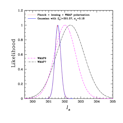
Figure 1: One-dimensional marginalized probability distributions of CMB shift parameter lasubscriptπ‘™π‘Žl_{a} derived from Planck, WMAP9, and WMAP7 data.
Refer to caption
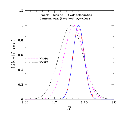
Figure 2: One-dimensional marginalized probability distribution of CMB shift parameter R𝑅R derived from Planck, WMAP9, and WMAP7 data.
Refer to caption
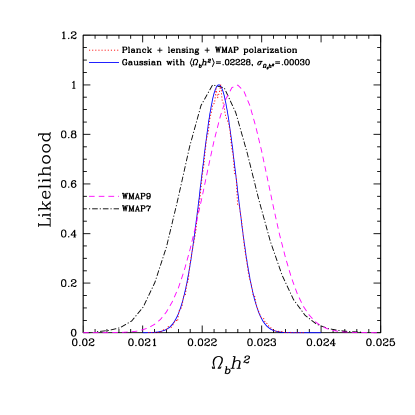
Figure 3: One-dimensional marginalized probability distribution of the dimensionless baryon density, Ο‰b≑Ωb​h2subscriptπœ”π‘subscriptΩ𝑏superscriptβ„Ž2\omega_{b}\equiv\Omega_{b}h^{2}, derived from Planck, WMAP9, and WMAP7 data.
Refer to caption
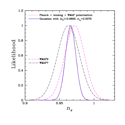
Figure 4: One-dimensional marginalized probability distributions of powerlaw index of primordial matter power spectrum, nssubscript𝑛𝑠n_{s}, derived from Planck, WMAP9, and WMAP7 data.

Figs.1-4 show the one-dimensional marginalized probability distributions (pdf) of (la,R,Ο‰b,ns)subscriptπ‘™π‘Žπ‘…subscriptπœ”π‘subscript𝑛𝑠(l_{a},R,\omega_{b},n_{s}) from Planck Ade et al. (2013), WMAP9 Bennett et al. (2012), and WMAP7 Komatsu et al. (2011) data, for wX​(z)=βˆ’1subscript𝑀𝑋𝑧1w_{X}(z)=-1 and one massive neutrino (with mass of 0.06eV), and without assuming a flat universe. We have used the Planck archiv data to obtain constraints on (la,R,Ο‰b,ns)subscriptπ‘™π‘Žπ‘…subscriptπœ”π‘subscript𝑛𝑠(l_{a},R,\omega_{b},n_{s}) from Planck and WMAP9; this archiv does not include wX​(z)β‰ βˆ’1subscript𝑀𝑋𝑧1w_{X}(z)\neq-1 cases without assuming a flat universe. Fortunately, the constraints on (la,R,Ο‰b,ns)subscriptπ‘™π‘Žπ‘…subscriptπœ”π‘subscript𝑛𝑠(l_{a},R,\omega_{b},n_{s}) (including the pdf’s) are not sensitive to the assumption about dark energy Wang, Chuang, & Mukherjee (2012). Three sets of pdf’s are shown in Figs.1-4:
(1) Planck+lensing+WP: Planck temperature data combined with Planck lensing, as well as WMAP polarization at low multipoles (l≀23𝑙23l\leq 23). This set represents the tightest constraints from CMB data only at present. Note that excluding the Planck lensing data changes the mean values of (la,R,Ο‰b,ns)subscriptπ‘™π‘Žπ‘…subscriptπœ”π‘subscript𝑛𝑠(l_{a},R,\omega_{b},n_{s}) by 0.2% or less, and increases the dispersions slightly.
(2) WMAP: WMAP 9 year temperature and polarization data.
(3) WMAP7: WMAP 7 year temperature and polarization data.

The Planck+lensing+WP pdf’s in Figs.1-4 are well fitted by Gaussian distributions with the following means and standard deviations:

⟨la⟩=301.57,σ​(la)=0.18formulae-sequencedelimited-⟨⟩subscriptπ‘™π‘Ž301.57𝜎subscriptπ‘™π‘Ž0.18\displaystyle\langle l_{a}\rangle=301.57,\sigma(l_{a})=0.18
⟨R⟩=1.7407,σ​(R)=0.0094formulae-sequencedelimited-βŸ¨βŸ©π‘…1.7407πœŽπ‘…0.0094\displaystyle\langle R\rangle=1.7407,\sigma(R)=0.0094
βŸ¨Ο‰b⟩=0.02228,σ​(Ο‰b)=0.00030formulae-sequencedelimited-⟨⟩subscriptπœ”π‘0.02228𝜎subscriptπœ”π‘0.00030\displaystyle\langle\omega_{b}\rangle=0.02228,\sigma(\omega_{b})=0.00030
⟨ns⟩=0.9662,σ​(ns)=0.0075.formulae-sequencedelimited-⟨⟩subscript𝑛𝑠0.9662𝜎subscript𝑛𝑠0.0075\displaystyle\langle n_{s}\rangle=0.9662,\sigma(n_{s})=0.0075. (12)

The normalized covariance matrix of (la,R,Ο‰b,ns)subscriptπ‘™π‘Žπ‘…subscriptπœ”π‘subscript𝑛𝑠(l_{a},R,\omega_{b},n_{s}) is

(1.00000.5250βˆ’0.4235βˆ’0.44750.52501.0000βˆ’0.6925βˆ’0.8240βˆ’0.4235βˆ’0.69251.00000.6109βˆ’0.4475βˆ’0.82400.61091.0000)1.00000.52500.42350.44750.52501.00000.69250.82400.42350.69251.00000.61090.44750.82400.61091.0000\left(\begin{array}[]{cccc}1.0000&0.5250&-0.4235&-0.4475\\ 0.5250&1.0000&-0.6925&-0.8240\\ -0.4235&-0.6925&1.0000&0.6109\\ -0.4475&-0.8240&0.6109&1.0000\\ \end{array}\right) (13)

For comparison, we have also obtained the WMAP9 constraints on (la,R,Ο‰b,ns)subscriptπ‘™π‘Žπ‘…subscriptπœ”π‘subscript𝑛𝑠(l_{a},R,\omega_{b},n_{s}). The WMAP9 in Figs.1-4 are well fitted by Gaussian distributions with the following means and standard deviations:

⟨la⟩=302.02,σ​(la)=0.66formulae-sequencedelimited-⟨⟩subscriptπ‘™π‘Ž302.02𝜎subscriptπ‘™π‘Ž0.66\displaystyle\langle l_{a}\rangle=302.02,\sigma(l_{a})=0.66
⟨R⟩=1.7327,σ​(R)=0.0164formulae-sequencedelimited-βŸ¨βŸ©π‘…1.7327πœŽπ‘…0.0164\displaystyle\langle R\rangle=1.7327,\sigma(R)=0.0164
βŸ¨Ο‰b⟩=0.02260,σ​(Ο‰b)=0.00053formulae-sequencedelimited-⟨⟩subscriptπœ”π‘0.02260𝜎subscriptπœ”π‘0.00053\displaystyle\langle\omega_{b}\rangle=0.02260,\sigma(\omega_{b})=0.00053
⟨ns⟩=0.9719,σ​(ns)=0.0143.formulae-sequencedelimited-⟨⟩subscript𝑛𝑠0.9719𝜎subscript𝑛𝑠0.0143\displaystyle\langle n_{s}\rangle=0.9719,\sigma(n_{s})=0.0143. (14)

The normalized covariance matrix of (la,R,Ο‰b,ns)subscriptπ‘™π‘Žπ‘…subscriptπœ”π‘subscript𝑛𝑠(l_{a},R,\omega_{b},n_{s}) is

(1.00000.3883βˆ’0.6089βˆ’0.53910.38831.0000βˆ’0.5239βˆ’0.6523βˆ’0.6089βˆ’0.52391.00000.8563βˆ’0.5391βˆ’0.65230.85631.0000)1.00000.38830.60890.53910.38831.00000.52390.65230.60890.52391.00000.85630.53910.65230.85631.0000\left(\begin{array}[]{cccc}1.0000&0.3883&-0.6089&-0.5391\\ 0.3883&1.0000&-0.5239&-0.6523\\ -0.6089&-0.5239&1.0000&0.8563\\ -0.5391&-0.6523&0.8563&1.0000\\ \end{array}\right) (15)

The WMAP7 constraints are from Wang, Chuang, & Mukherjee (2012).

Since the primary GC data we use in this paper have been marginalized over nssubscript𝑛𝑠n_{s} CW12 , we should marginalize the CMB distance priors over nssubscript𝑛𝑠n_{s} as well.222An improved approach is to use GC data that retain the nssubscript𝑛𝑠n_{s} dependence, and combine with the CMB constraints on (la,R,Ο‰b,ns)subscriptπ‘™π‘Žπ‘…subscriptπœ”π‘subscript𝑛𝑠(l_{a},R,\omega_{b},n_{s}). This means dropping the 4th row and 4th column from the normalized covariance matrix of (la,R,Ο‰b,ns)subscriptπ‘™π‘Žπ‘…subscriptπœ”π‘subscript𝑛𝑠(l_{a},R,\omega_{b},n_{s}), then obtain the covariance matrix for (la,R,Ο‰b)subscriptπ‘™π‘Žπ‘…subscriptπœ”π‘(l_{a},R,\omega_{b}) as follows:

CovC​M​B​(pi,pj)=σ​(pi)​σ​(pj)​NormCovC​M​B​(pi,pj),subscriptCov𝐢𝑀𝐡subscript𝑝𝑖subscriptπ‘π‘—πœŽsubscriptπ‘π‘–πœŽsubscript𝑝𝑗subscriptNormCov𝐢𝑀𝐡subscript𝑝𝑖subscript𝑝𝑗\mbox{Cov}_{CMB}(p_{i},p_{j})=\sigma(p_{i})\,\sigma(p_{j})\,\mbox{NormCov}_{CMB}(p_{i},p_{j}), (16)

where i,j=1,2,3formulae-sequence𝑖𝑗123i,j=1,2,3. The rms variance σ​(pi)𝜎subscript𝑝𝑖\sigma(p_{i}) and the normalized covariance matrix NormCovC​M​BsubscriptNormCov𝐢𝑀𝐡\mbox{NormCov}_{CMB} are given by Eqs.(12) and (13) for Planck+lensing+WP, and Eqs.(14) and (15) for WMAP9 respectively.

CMB data are included in our analysis by adding the following term to the Ο‡2superscriptπœ’2\chi^{2} of a given model with p1=la​(zβˆ—)subscript𝑝1subscriptπ‘™π‘Žsubscript𝑧p_{1}=l_{a}(z_{*}), p2=R​(zβˆ—)subscript𝑝2𝑅subscript𝑧p_{2}=R(z_{*}),and p3=Ο‰bsubscript𝑝3subscriptπœ”π‘p_{3}=\omega_{b}:

Ο‡C​M​B2=Δ​pi​[CovC​M​Bβˆ’1​(pi,pj)]​Δ​pj,Δ​pi=piβˆ’pid​a​t​a,formulae-sequencesubscriptsuperscriptπœ’2𝐢𝑀𝐡Δsubscript𝑝𝑖delimited-[]subscriptsuperscriptCov1𝐢𝑀𝐡subscript𝑝𝑖subscript𝑝𝑗Δsubscript𝑝𝑗Δsubscript𝑝𝑖subscript𝑝𝑖superscriptsubscriptπ‘π‘–π‘‘π‘Žπ‘‘π‘Ž\chi^{2}_{CMB}=\Delta p_{i}\left[\mbox{Cov}^{-1}_{CMB}(p_{i},p_{j})\right]\Delta p_{j},\hskip 14.22636pt\Delta p_{i}=p_{i}-p_{i}^{data}, (17)

where pid​a​t​asuperscriptsubscriptπ‘π‘–π‘‘π‘Žπ‘‘π‘Žp_{i}^{data} are the mean from Eq.(12) and Eq.(14), and CovC​M​Bβˆ’1subscriptsuperscriptCov1𝐢𝑀𝐡{\rm Cov}^{-1}_{CMB} is the inverse of the covariance matrix of [la(zβˆ—),R(zβˆ—),Ο‰b]l_{a}(z_{*}),R(z_{*}),\omega_{b}] from Eq.(16). Note that p4=nssubscript𝑝4subscript𝑛𝑠p_{4}=n_{s} should be added if the constraints on nssubscript𝑛𝑠n_{s} are included in the GC data.

II.2 Analysis of SN Ia Data

SN Ia data give measurements of the luminosity distance dL​(z)subscript𝑑𝐿𝑧d_{L}(z) through that of the distance modulus of each SN:

ΞΌ0≑mβˆ’M=5​log⁑[dL​(z)Mpc]+25,subscriptπœ‡0π‘šπ‘€5subscript𝑑𝐿𝑧Mpc25\mu_{0}\equiv m-M=5\log\left[\frac{d_{L}(z)}{\mathrm{Mpc}}\right]+25, (18)

where mπ‘šm and M𝑀M represent the apparent and absolute magnitude of a SN. The luminosity distance dL​(z)=(1+z)​r​(z)subscript𝑑𝐿𝑧1π‘§π‘Ÿπ‘§d_{L}(z)=(1+z)\,r(z), with the comoving distance r​(z)π‘Ÿπ‘§r(z) given by Eq.(1).

Care must be taken in interpreting supernova distances in an inhomogeneous universe Clarkson11 . We use the compilation of SN Ia data by Conley et al. (2011) Conley11 , which include the SNe Ia from the first three years of the Supernova Legacy Survey (SNLS3), the largest homogeneous SN Ia data set publicly available at present, and apply flux-averaging to reduce the systematic bias due to weak lensing magnification of SNe Wang (2000); Wang & Mukherjee (2004); Wang (2005), as detailed in Wang, Chuang, & Mukherjee (2012) Wang, Chuang, & Mukherjee (2012).

For a set of 472 SNe Ia, Conley et al. (2011) Conley11 give the apparent B𝐡B magnitude, mBsubscriptπ‘šπ΅m_{B}, and the covariance matrix for Δ​m≑mBβˆ’mmodΞ”π‘šsubscriptπ‘šπ΅subscriptπ‘šmod\Delta m\equiv m_{B}-m_{\rm mod}, with

mmod=5​log10β‘π’ŸL​(z|s)βˆ’Ξ±β€‹(sβˆ’1)+Ξ²β€‹π’ž+β„³,subscriptπ‘šmod5subscript10subscriptπ’ŸπΏconditional𝑧s𝛼𝑠1π›½π’žβ„³m_{\rm mod}=5\log_{10}{\cal D}_{L}(z|\mbox{\bf s})-\alpha(s-1)+\beta{\cal C}+{\cal M}, (19)

where π’ŸL​(z|s)subscriptπ’ŸπΏconditional𝑧s{\cal D}_{L}(z|\mbox{\bf s}) is the luminosity distance multiplied by H0subscript𝐻0H_{0} for a given set of cosmological parameters {𝐬}𝐬\{{\bf s}\}, s𝑠s is the stretch measure of the SN light curve shape, and π’žπ’ž{\cal C} is the color measure for the SN. β„³β„³{\cal M} is a nuisance parameter representing some combination of the absolute magnitude of a fiducial SN Ia, M𝑀M, and the Hubble constant H0subscript𝐻0H_{0}. Since the time dilation part of the observed luminosity distance depends on the total redshift zhelsubscript𝑧helz_{\rm hel} (special relativistic plus cosmological), we have Hui06

π’ŸL​(z|s)≑cβˆ’1​H0​(1+zhel)​r​(z|s),subscriptπ’ŸπΏconditional𝑧ssuperscript𝑐1subscript𝐻01subscript𝑧helπ‘Ÿconditional𝑧s{\cal D}_{L}(z|\mbox{\bf s})\equiv c^{-1}H_{0}(1+z_{\rm hel})r(z|\mbox{\bf s}), (20)

where z𝑧z and zhelsubscript𝑧helz_{\rm hel} are the CMB restframe and heliocentric redshifts of the SN.

For a set of N𝑁N SNe with correlated errors, we have Conley11

Ο‡2=Δ​mTβ‹…Cβˆ’1⋅Δ​msuperscriptπœ’2β‹…Ξ”superscriptm𝑇superscriptC1Ξ”m\chi^{2}=\Delta\mbox{\bf m}^{T}\cdot\mbox{\bf C}^{-1}\cdot\Delta\mbox{\bf m} (21)

where Δ​𝐦Δ𝐦\Delta\bf m is a vector with N𝑁N components, and C is the NΓ—N𝑁𝑁N\times N covariance matrix of the SNe Ia.

Note that Δ​mΞ”π‘š\Delta m is equivalent to Δ​μ0Ξ”subscriptπœ‡0\Delta\mu_{0}, since

Δ​m≑mBβˆ’mmod=[mB+α​(sβˆ’1)βˆ’Ξ²β€‹π’ž]βˆ’β„³.Ξ”π‘šsubscriptπ‘šπ΅subscriptπ‘šmoddelimited-[]subscriptπ‘šπ΅π›Όπ‘ 1π›½π’žβ„³\Delta m\equiv m_{B}-m_{\rm mod}=\left[m_{B}+\alpha(s-1)-\beta{\cal C}\right]-{\cal M}. (22)

The total covariance matrix is Conley11

C=Dstat+Cstat+Csys,CsubscriptDstatsubscriptCstatsubscriptCsys\mbox{\bf C}=\mbox{\bf D}_{\rm stat}+\mbox{\bf C}_{\rm stat}+\mbox{\bf C}_{\rm sys}, (23)

with the diagonal part of the statistical uncertainty given by Conley11

Dstat,iisubscriptDstatii\displaystyle\mbox{\bf D}_{\rm stat,ii} =\displaystyle= ΟƒmB,i2+Οƒint2+Οƒlensing2+Οƒhost​correction2subscriptsuperscript𝜎2subscriptπ‘šπ΅π‘–subscriptsuperscript𝜎2intsubscriptsuperscript𝜎2lensingsubscriptsuperscript𝜎2hostcorrection\displaystyle\sigma^{2}_{m_{B},i}+\sigma^{2}_{\rm int}+\sigma^{2}_{\rm lensing}+\sigma^{2}_{{\rm host}\,{\rm correction}} (24)
+[5​(1+zi)zi​(1+zi/2)​ln⁑10]2​σz,i2+Ξ±2​σs,i2+Ξ²2β€‹Οƒπ’ž,i2superscriptdelimited-[]51subscript𝑧𝑖subscript𝑧𝑖1subscript𝑧𝑖2102subscriptsuperscript𝜎2𝑧𝑖superscript𝛼2subscriptsuperscript𝜎2𝑠𝑖superscript𝛽2subscriptsuperscript𝜎2π’žπ‘–\displaystyle+\left[\frac{5(1+z_{i})}{z_{i}(1+z_{i}/2)\ln 10}\right]^{2}\sigma^{2}_{z,i}+\alpha^{2}\sigma^{2}_{s,i}+\beta^{2}\sigma^{2}_{{\cal C},i}
+2​α​CmB​s,iβˆ’2​β​CmBβ€‹π’ž,iβˆ’2​α​β​Csβ€‹π’ž,i,2𝛼subscript𝐢subscriptπ‘šπ΅π‘ π‘–2𝛽subscript𝐢subscriptπ‘šπ΅π’žπ‘–2𝛼𝛽subscriptπΆπ‘ π’žπ‘–\displaystyle+2\alpha C_{m_{B}s,i}-2\beta C_{m_{B}{\cal C},i}-2\alpha\beta C_{s{\cal C},i},

where CmB​s,isubscript𝐢subscriptπ‘šπ΅π‘ π‘–C_{m_{B}s,i}, CmBβ€‹π’ž,isubscript𝐢subscriptπ‘šπ΅π’žπ‘–C_{m_{B}{\cal C},i}, and Csβ€‹π’ž,isubscriptπΆπ‘ π’žπ‘–C_{s{\cal C},i} are the covariances between mBsubscriptπ‘šπ΅m_{B}, s𝑠s, and π’žπ’ž{\cal C} for the i𝑖i-th SN. Note also that Οƒz,i2subscriptsuperscript𝜎2𝑧𝑖\sigma^{2}_{z,i} includes a peculiar velocity residual of 0.0005 (i.e., 150 km/s) added in quadrature Conley11 .

The statistical and systematic covariance matrices, CstatsubscriptCstat\mbox{\bf C}_{\rm stat} and CsyssubscriptCsys\mbox{\bf C}_{\rm sys}, are generally not diagonal Conley11 , and are given in the form:

Cstat+Csys=V0+Ξ±2​Va+Ξ²2​Vb+2​α​V0​aβˆ’2​β​V0​bβˆ’2​α​β​Va​b.subscriptCstatsubscriptCsyssubscript𝑉0superscript𝛼2subscriptπ‘‰π‘Žsuperscript𝛽2subscript𝑉𝑏2𝛼subscript𝑉0π‘Ž2𝛽subscript𝑉0𝑏2𝛼𝛽subscriptπ‘‰π‘Žπ‘\mbox{\bf C}_{\rm stat}+\mbox{\bf C}_{\rm sys}=V_{0}+\alpha^{2}V_{a}+\beta^{2}V_{b}+2\alpha V_{0a}-2\beta V_{0b}-2\alpha\beta V_{ab}. (25)

where V0subscript𝑉0V_{0}, Vasubscriptπ‘‰π‘ŽV_{a}, Vbsubscript𝑉𝑏V_{b}, V0​asubscript𝑉0π‘ŽV_{0a}, V0​bsubscript𝑉0𝑏V_{0b}, and Va​bsubscriptπ‘‰π‘Žπ‘V_{ab} are matrices given by the SNLS data archive at https://tspace.library.utoronto.ca/handle/1807/24512/. CstatsubscriptCstat\mbox{\bf C}_{\rm stat} includes the uncertainty in the SN model. CsyssubscriptCsys\mbox{\bf C}_{\rm sys} includes the uncertainty in the zero point. Note that CstatsubscriptCstat\mbox{\bf C}_{\rm stat} and CsyssubscriptCsys\mbox{\bf C}_{\rm sys} do not depend on β„³β„³{\cal M}, since the relative distance moduli are independent of the value of β„³β„³{\cal M} Conley11 .

We refer the reader to Conley et al. (2011) Conley11 for a detailed discussion of the origins of the statistical and systematic errors. As an example, we note that the correlation of errors on different SNe arises from a statistical uncertainty in the zero point of one passband, e.g., rMsubscriptπ‘Ÿπ‘€r_{M}. This directly affects all SNe with rMsubscriptπ‘Ÿπ‘€r_{M} measurements due to K-corrections (restframe B𝐡B to rMsubscriptπ‘Ÿπ‘€r_{M}), and indirectly affects even the SNe without rMsubscriptπ‘Ÿπ‘€r_{M} measurements through the empirical SN models by changing the templates and the measured color-luminosity relationship.

For Ο‡2superscriptπœ’2\chi^{2} statistics using MCMC or a grid of parameters, here are the steps in flux-averaging Wang, Chuang, & Mukherjee (2012):

(1) Convert the distance modulus of SNe Ia into β€œfluxes”,

F​(zl)≑10βˆ’(ΞΌ0data​(zl)βˆ’25)/2.5=(dLdata​(zl)Mpc)βˆ’2.𝐹subscript𝑧𝑙superscript10superscriptsubscriptπœ‡0datasubscript𝑧𝑙252.5superscriptsuperscriptsubscript𝑑𝐿datasubscript𝑧𝑙Mpc2F(z_{l})\equiv 10^{-(\mu_{0}^{\rm data}(z_{l})-25)/2.5}=\left(\frac{d_{L}^{\rm data}(z_{l})}{\mbox{Mpc}}\right)^{-2}. (26)

(2) For a given set of cosmological parameters {𝐬}𝐬\{{\bf s}\}, obtain β€œabsolute luminosities”, {ℒ​(zl)β„’subscript𝑧𝑙{\cal L}(z_{l})}, by removing the redshift dependence of the β€œfluxes”, i.e.,

ℒ​(zl)≑dL2​(zl|𝐬)​F​(zl).β„’subscript𝑧𝑙superscriptsubscript𝑑𝐿2conditionalsubscript𝑧𝑙𝐬𝐹subscript𝑧𝑙{\cal L}(z_{l})\equiv d_{L}^{2}(z_{l}|{\bf s})\,F(z_{l}). (27)

(3) Flux-average the β€œabsolute luminosities” {β„’lisubscriptsuperscriptℒ𝑖𝑙{\cal L}^{i}_{l}} in each redshift bin i𝑖i to obtain {β„’Β―i}superscript¯ℒ𝑖\left\{\overline{\cal L}^{i}\right\}:

β„’Β―i=1Niβ€‹βˆ‘l=1Niβ„’li​(zl(i)),ziΒ―=1Niβ€‹βˆ‘l=1Nizl(i).formulae-sequencesuperscript¯ℒ𝑖1subscript𝑁𝑖superscriptsubscript𝑙1subscript𝑁𝑖subscriptsuperscriptℒ𝑖𝑙subscriptsuperscript𝑧𝑖𝑙¯subscript𝑧𝑖1subscript𝑁𝑖superscriptsubscript𝑙1subscript𝑁𝑖subscriptsuperscript𝑧𝑖𝑙\overline{\cal L}^{i}=\frac{1}{N_{i}}\sum_{l=1}^{N_{i}}{\cal L}^{i}_{l}(z^{(i)}_{l}),\hskip 28.45274pt\overline{z_{i}}=\frac{1}{N_{i}}\sum_{l=1}^{N_{i}}z^{(i)}_{l}. (28)

(4) Place β„’Β―isuperscript¯ℒ𝑖\overline{\cal L}^{i} at the mean redshift zΒ―isubscript¯𝑧𝑖\overline{z}_{i} of the i𝑖i-th redshift bin, now the binned flux is

F¯​(zΒ―i)=β„’Β―i/dL2​(zΒ―i|s).¯𝐹subscript¯𝑧𝑖superscript¯ℒ𝑖superscriptsubscript𝑑𝐿2conditionalsubscript¯𝑧𝑖s\overline{F}(\overline{z}_{i})=\overline{\cal L}^{i}/d_{L}^{2}(\overline{z}_{i}|\mbox{\bf s}). (29)

(5) Compute the covariance matrix of F¯​(zΒ―i)¯𝐹subscript¯𝑧𝑖\overline{F}(\overline{z}_{i}) and F¯​(zΒ―j)¯𝐹subscript¯𝑧𝑗\overline{F}(\overline{z}_{j}):

Cov​[F¯​(zΒ―i),F¯​(zΒ―j)]Cov¯𝐹subscript¯𝑧𝑖¯𝐹subscript¯𝑧𝑗\displaystyle\mbox{Cov}\left[\overline{F}(\overline{z}_{i}),\overline{F}(\overline{z}_{j})\right]
=\displaystyle= 1Ni​Nj[ln⁑10/2.5dL​(zΒ―i|s)​dL​(zΒ―j|s)]2β‹…\displaystyle\frac{1}{N_{i}N_{j}}\left[\frac{\ln 10/2.5}{d_{L}(\overline{z}_{i}|\mbox{\bf s})d_{L}(\overline{z}_{j}|\mbox{\bf s})}\right]^{2}\cdot
βˆ‘l=1Niβˆ‘m=1Njℒ​(zl(i))​ℒ​(zm(j))β€‹βŸ¨Ξ”β€‹ΞΌ0data​(zl(i))​Δ​μ0data​(zm(j))⟩superscriptsubscript𝑙1subscript𝑁𝑖superscriptsubscriptπ‘š1subscript𝑁𝑗ℒsuperscriptsubscript𝑧𝑙𝑖ℒsuperscriptsubscriptπ‘§π‘šπ‘—delimited-βŸ¨βŸ©Ξ”superscriptsubscriptπœ‡0datasuperscriptsubscript𝑧𝑙𝑖Δsuperscriptsubscriptπœ‡0datasuperscriptsubscriptπ‘§π‘šπ‘—\displaystyle\sum_{l=1}^{N_{i}}\sum_{m=1}^{N_{j}}{\cal L}(z_{l}^{(i)}){\cal L}(z_{m}^{(j)})\langle\Delta\mu_{0}^{\rm data}(z_{l}^{(i)})\Delta\mu_{0}^{\rm data}(z_{m}^{(j)})\rangle

where βŸ¨Ξ”β€‹ΞΌ0data​(zl(i))​Δ​μ0data​(zm(j))⟩delimited-βŸ¨βŸ©Ξ”superscriptsubscriptπœ‡0datasuperscriptsubscript𝑧𝑙𝑖Δsuperscriptsubscriptπœ‡0datasuperscriptsubscriptπ‘§π‘šπ‘—\langle\Delta\mu_{0}^{\rm data}(z_{l}^{(i)})\Delta\mu_{0}^{\rm data}(z_{m}^{(j)})\rangle is the covariance of the measured distance moduli of the l𝑙l-th SN Ia in the i𝑖i-th redshift bin, and the mπ‘šm-th SN Ia in the j𝑗j-th redshift bin. ℒ​(z)ℒ𝑧{\cal L}(z) is defined by Eqs.(26) and (27).

(6) For the flux-averaged data, {F¯​(zΒ―i)}¯𝐹subscript¯𝑧𝑖\left\{\overline{F}(\overline{z}_{i})\right\}, compute

Ο‡2=βˆ‘i​jΔ​F¯​(zΒ―i)​Covβˆ’1​[F¯​(zΒ―i),F¯​(zΒ―j)]​Δ​F¯​(zΒ―j)superscriptπœ’2subscript𝑖𝑗Δ¯𝐹subscript¯𝑧𝑖superscriptCov1¯𝐹subscript¯𝑧𝑖¯𝐹subscript¯𝑧𝑗Δ¯𝐹subscript¯𝑧𝑗\chi^{2}=\sum_{ij}\Delta\overline{F}(\overline{z}_{i})\,\mbox{Cov}^{-1}\left[\overline{F}(\overline{z}_{i}),\overline{F}(\overline{z}_{j})\right]\,\Delta\overline{F}(\overline{z}_{j}) (31)

where

Δ​F¯​(zΒ―i)≑F¯​(zΒ―i)βˆ’Fp​(zΒ―i|s),Δ¯𝐹subscript¯𝑧𝑖¯𝐹subscript¯𝑧𝑖superscript𝐹𝑝conditionalsubscript¯𝑧𝑖s\Delta\overline{F}(\overline{z}_{i})\equiv\overline{F}(\overline{z}_{i})-F^{p}(\overline{z}_{i}|\mbox{\bf s}), (32)

with Fp​(zΒ―i|s)=(dL​(z|s)/Mpc)βˆ’2superscript𝐹𝑝conditionalsubscript¯𝑧𝑖ssuperscriptsubscript𝑑𝐿conditional𝑧sMpc2F^{p}(\overline{z}_{i}|\mbox{\bf s})=\left(d_{L}(z|\mbox{\bf s})/\mbox{Mpc}\right)^{-2}.

For the sample of SNe we use in this study, we flux-averaged the SNe with d​z=0.04𝑑𝑧0.04dz=0.04, to ensure that almost all redshift bins contain at least one SN. Our SN flux-averaging code is available at http://www.nhn.ou.edu/∼similar-to\simwang/SNcode/.

II.3 Galaxy Clustering Data

For GC data, we use the measurements of H​(z)​rs​(zd)/c𝐻𝑧subscriptπ‘Ÿπ‘ subscript𝑧𝑑𝑐H(z)r_{s}(z_{d})/c and DA​(z)/rs​(zd)subscript𝐷𝐴𝑧subscriptπ‘Ÿπ‘ subscript𝑧𝑑D_{A}(z)/r_{s}(z_{d}) (where H​(z)𝐻𝑧H(z) is the Hubble parameter, DA​(z)subscript𝐷𝐴𝑧D_{A}(z) is the angular diameter distance, and rs​(zd)subscriptπ‘Ÿπ‘ subscript𝑧𝑑r_{s}(z_{d}) is the sound horizon at the drag epoch) from the two-dimensional two-point correlation function measured at z=0.35 CW12 and z=0.57 Chuang et al. (2013). The z=0.35𝑧0.35z=0.35 measurement was made by Chuang & Wang (2012) CW12 using a sample of the SDSS DR7 Luminous Red Galaxies (LRGs). The z=0.57𝑧0.57z=0.57 measurement was made by Chuang et al. (2013) Chuang et al. (2013) using the CMASS galaxy sample from BOSS.

Using the two-dimensional two-point correlation function of SDSS DR7 in the scale range of 40-120 Mpc/hβ„Žh, Chuang & Wang (2012) CW12 found that

H​(z=0.35)​rs​(zd)/c𝐻𝑧0.35subscriptπ‘Ÿπ‘ subscript𝑧𝑑𝑐\displaystyle H(z=0.35)r_{s}(z_{d})/c =\displaystyle= 0.0434Β±0.0018plus-or-minus0.04340.0018\displaystyle 0.0434\pm 0.0018
DA​(z=0.35)/rs​(zd)subscript𝐷𝐴𝑧0.35subscriptπ‘Ÿπ‘ subscript𝑧𝑑\displaystyle D_{A}(z=0.35)/r_{s}(z_{d}) =\displaystyle= 6.60Β±0.26plus-or-minus6.600.26\displaystyle 6.60\pm 0.26
rπ‘Ÿ\displaystyle r =\displaystyle= 0.06040.0604\displaystyle 0.0604 (33)

where rπ‘Ÿr is the normalized correlation coefficient between H​(z=0.35)​rs​(zd)/c𝐻𝑧0.35subscriptπ‘Ÿπ‘ subscript𝑧𝑑𝑐H(z=0.35)r_{s}(z_{d})/c and DA​(z=0.35)/rs​(zd)subscript𝐷𝐴𝑧0.35subscriptπ‘Ÿπ‘ subscript𝑧𝑑D_{A}(z=0.35)/r_{s}(z_{d}), and rs​(zd)subscriptπ‘Ÿπ‘ subscript𝑧𝑑r_{s}(z_{d}) is the sound horizon at the drag epoch (given by Eqs.(5) and (9).

In a similar analysis using the CMASS galaxy sample from BOSS, Chuang et al. (2013) found that

H​(z=0.57)​rs​(zd)/c𝐻𝑧0.57subscriptπ‘Ÿπ‘ subscript𝑧𝑑𝑐\displaystyle H(z=0.57)r_{s}(z_{d})/c =\displaystyle= 0.0454Β±0.0031plus-or-minus0.04540.0031\displaystyle 0.0454\pm 0.0031
DA​(z=0.57)/rs​(zd)subscript𝐷𝐴𝑧0.57subscriptπ‘Ÿπ‘ subscript𝑧𝑑\displaystyle D_{A}(z=0.57)/r_{s}(z_{d}) =\displaystyle= 8.95Β±0.27plus-or-minus8.950.27\displaystyle 8.95\pm 0.27
rπ‘Ÿ\displaystyle r =\displaystyle= 0.48740.4874\displaystyle 0.4874 (34)

We marginalize over the growth rate measurement made by Chuang et al. 2013 Chuang et al. (2013) for a conservative approach.

GC data are included in our analysis by adding Ο‡G​C2=Ο‡G​C​12+Ο‡G​C​22subscriptsuperscriptπœ’2𝐺𝐢subscriptsuperscriptπœ’2𝐺𝐢1subscriptsuperscriptπœ’2𝐺𝐢2\chi^{2}_{GC}=\chi^{2}_{GC1}+\chi^{2}_{GC2}, with zG​C​1=0.35subscript𝑧𝐺𝐢10.35z_{GC1}=0.35 and zG​C​2=0.57subscript𝑧𝐺𝐢20.57z_{GC2}=0.57, to the Ο‡2superscriptπœ’2\chi^{2} of a given model. Note that

Ο‡G​C​i2=Δ​pi​[CG​Cβˆ’1​(pi,pj)]​Δ​pj,Δ​pi=piβˆ’pid​a​t​a,formulae-sequencesubscriptsuperscriptπœ’2𝐺𝐢𝑖Δsubscript𝑝𝑖delimited-[]subscriptsuperscriptC1𝐺𝐢subscript𝑝𝑖subscript𝑝𝑗Δsubscript𝑝𝑗Δsubscript𝑝𝑖subscript𝑝𝑖superscriptsubscriptπ‘π‘–π‘‘π‘Žπ‘‘π‘Ž\chi^{2}_{GCi}=\Delta p_{i}\left[{\rm C}^{-1}_{GC}(p_{i},p_{j})\right]\Delta p_{j},\hskip 14.22636pt\Delta p_{i}=p_{i}-p_{i}^{data}, (35)

where p1=H​(zG​C​i)​rs​(zd)/csubscript𝑝1𝐻subscript𝑧𝐺𝐢𝑖subscriptπ‘Ÿπ‘ subscript𝑧𝑑𝑐p_{1}=H(z_{GCi})r_{s}(z_{d})/c and p2=DA​(zG​C​i)/rs​(zd)subscript𝑝2subscript𝐷𝐴subscript𝑧𝐺𝐢𝑖subscriptπ‘Ÿπ‘ subscript𝑧𝑑p_{2}=D_{A}(z_{GCi})/r_{s}(z_{d}), with i=1,2𝑖12i=1,2.

II.4 Gammay-ray Burst Data

We add gammay-ray burst (GRB) data to our analysis, since these are complementary in redshift range to the SN Ia data. We use GRB data in the form of the model-independent GRB distance measurements from Wang (2008c) Wang08c , which were derived from the data of 69 GRBs with 0.17≀z≀6.60.17𝑧6.60.17\leq z\leq 6.6 from Schaefer (2007) Schaefer07 333The proper calibration of GRBs is an active area of research. For recent studies on the impact of detector thresholds, spectral analysis, and unknown selection effects, see, e.g., Butler07 ; Butler09 ; Petrosian09 ; Shahmoradi11 ..

The GRB distance measurements are given in terms of Wang08c

rp¯​(zi)≑rp​(z)rp​(0.17),rp​(z)≑(1+z)1/2z​H0c​h​r​(z),formulae-sequenceΒ―subscriptπ‘Ÿπ‘subscript𝑧𝑖subscriptπ‘Ÿπ‘π‘§subscriptπ‘Ÿπ‘0.17subscriptπ‘Ÿπ‘π‘§superscript1𝑧12𝑧subscript𝐻0π‘β„Žπ‘Ÿπ‘§\overline{r_{p}}(z_{i})\equiv\frac{r_{p}(z)}{r_{p}(0.17)},\hskip 28.45274ptr_{p}(z)\equiv\frac{(1+z)^{1/2}}{z}\,\frac{H_{0}}{ch}\,r(z), (36)

where r​(z)π‘Ÿπ‘§r(z) is the comoving distance at z𝑧z.

The GRB data are included in our analysis by adding the following term to the Ο‡2superscriptπœ’2\chi^{2} of a given model:

Ο‡G​R​B2subscriptsuperscriptπœ’2𝐺𝑅𝐡\displaystyle\chi^{2}_{GRB} =\displaystyle= [Δ​rp¯​(zi)]β‹…(CovG​R​Bβˆ’1)i​jβ‹…[Δ​rp¯​(zj)]β‹…delimited-[]Δ¯subscriptπ‘Ÿπ‘subscript𝑧𝑖subscriptsubscriptsuperscriptCov1𝐺𝑅𝐡𝑖𝑗delimited-[]Δ¯subscriptπ‘Ÿπ‘subscript𝑧𝑗\displaystyle\left[\Delta\overline{r_{p}}(z_{i})\right]\cdot\left(\mathrm{Cov}^{-1}_{GRB}\right)_{ij}\cdot\left[\Delta\overline{r_{p}}(z_{j})\right]
Δ​rp¯​(zi)Δ¯subscriptπ‘Ÿπ‘subscript𝑧𝑖\displaystyle\Delta\overline{r_{p}}(z_{i}) =\displaystyle= rpΒ―data​(zi)βˆ’rp¯​(zi),superscriptΒ―subscriptπ‘Ÿπ‘datasubscript𝑧𝑖¯subscriptπ‘Ÿπ‘subscript𝑧𝑖\displaystyle\overline{r_{p}}^{\mathrm{data}}(z_{i})-\overline{r_{p}}(z_{i}), (37)

where rp¯​(z)Β―subscriptπ‘Ÿπ‘π‘§\overline{r_{p}}(z) is defined by Eq.(36). The covariance matrix is given by

(CovG​R​B)i​j=σ​(rp¯​(zi))​σ​(rp¯​(zj))​(CovΒ―G​R​B)i​j,subscriptsubscriptCovπΊπ‘…π΅π‘–π‘—πœŽΒ―subscriptπ‘Ÿπ‘subscriptπ‘§π‘–πœŽΒ―subscriptπ‘Ÿπ‘subscript𝑧𝑗subscriptsubscriptΒ―Cov𝐺𝑅𝐡𝑖𝑗\left(\mathrm{Cov}_{GRB}\right)_{ij}=\sigma(\overline{r_{p}}(z_{i}))\sigma(\overline{r_{p}}(z_{j}))\left(\overline{\mathrm{Cov}}_{GRB}\right)_{ij}, (38)

where CovΒ―G​R​BsubscriptΒ―Cov𝐺𝑅𝐡\overline{\mathrm{Cov}}_{GRB} is the normalized covariance matrix from Table 3 of Wang (2008c) Wang08c , and

σ​(rp¯​(zi))𝜎¯subscriptπ‘Ÿπ‘subscript𝑧𝑖\displaystyle\sigma(\overline{r_{p}}(z_{i})) =\displaystyle= σ​(rp¯​(zi))+,if​rp¯​(z)β‰₯rp¯​(z)data;𝜎superscriptΒ―subscriptπ‘Ÿπ‘subscript𝑧𝑖ifΒ―subscriptπ‘Ÿπ‘π‘§Β―subscriptπ‘Ÿπ‘superscript𝑧data\displaystyle\sigma\left(\overline{r_{p}}(z_{i})\right)^{+},\hskip 14.22636pt\mathrm{if}\,\,\overline{r_{p}}(z)\geq\overline{r_{p}}(z)^{\mathrm{data}};
σ​(rp¯​(zi))𝜎¯subscriptπ‘Ÿπ‘subscript𝑧𝑖\displaystyle\sigma(\overline{r_{p}}(z_{i})) =\displaystyle= σ​(rp¯​(zi))βˆ’,if​rp¯​(z)<rp¯​(z)data,𝜎superscriptΒ―subscriptπ‘Ÿπ‘subscript𝑧𝑖ifΒ―subscriptπ‘Ÿπ‘π‘§Β―subscriptπ‘Ÿπ‘superscript𝑧data\displaystyle\sigma\left(\overline{r_{p}}(z_{i})\right)^{-},\hskip 14.22636pt\mathrm{if}\,\,\overline{r_{p}}(z)<\overline{r_{p}}(z)^{\mathrm{data}}, (39)

where σ​(rp¯​(zi))+𝜎superscriptΒ―subscriptπ‘Ÿπ‘subscript𝑧𝑖\sigma\left(\overline{r_{p}}(z_{i})\right)^{+} and σ​(rp¯​(zi))βˆ’πœŽsuperscriptΒ―subscriptπ‘Ÿπ‘subscript𝑧𝑖\sigma\left(\overline{r_{p}}(z_{i})\right)^{-} are the 68% C.L. errors given in Table 2 of Wang (2008c) Wang08c .

II.5 Dark energy parametrization

Since we are ignorant of the true nature of dark energy, it is useful to measure the dark energy density function X​(z)≑ρX​(z)/ρX​(0)𝑋𝑧subscriptπœŒπ‘‹π‘§subscriptπœŒπ‘‹0X(z)\equiv\rho_{X}(z)/\rho_{X}(0) as a free function of redshift Wang & Garnavich (2001); Wang & Tegmark (2004); Wang & Freese (2006). This has the advantage of allowing dark energy models in which ρX​(z)subscriptπœŒπ‘‹π‘§\rho_{X}(z) becomes negative in the future, e.g., the β€œBig Crunch” models Linde (1987); WangLinde04 , which are precluded if we parametrize dark energy with an equation of state wX​(z)subscript𝑀𝑋𝑧w_{X}(z) Wang & Tegmark (2004).

Here we parametrize X​(z)𝑋𝑧X(z) by cubic-splining its values at z=1/3𝑧13z=1/3, 2/3232/3, and 1.0, and assume that X​(z>1)=X​(z=1)𝑋𝑧1𝑋𝑧1X(z>1)=X(z=1). For simplicity of notation, we define X0.33≑X​(z=1/3)subscript𝑋0.33𝑋𝑧13X_{0.33}\equiv X(z=1/3), X0.67≑X​(z=2/3)subscript𝑋0.67𝑋𝑧23X_{0.67}\equiv X(z=2/3), and X1.0≑X​(z=1)subscript𝑋1.0𝑋𝑧1X_{1.0}\equiv X(z=1). Fixing X​(z>1)𝑋𝑧1X(z>1) reflects the limit of current data, and avoids making assumptions about early dark energy that can be propagated into artificial constraints on dark energy at low z𝑧z Wang & Tegmark (2004); Wang & Mukherjee (2007).

For comparison with the work of others, we also consider a dark energy equation of state linear in the cosmic scale factor aπ‘Ža, wX​(a)=w0+(1βˆ’a)​wasubscriptπ‘€π‘‹π‘Žsubscript𝑀01π‘Žsubscriptπ‘€π‘Žw_{X}(a)=w_{0}+(1-a)w_{a} Chev01 (2001). A related parametrization is Wang08b

wX​(z)=w0​(3​aβˆ’2)+3​w0.5​(1βˆ’a),subscript𝑀𝑋𝑧subscript𝑀03π‘Ž23subscript𝑀0.51π‘Žw_{X}(z)=w_{0}(3a-2)+3w_{0.5}(1-a), (40)

where w0.5≑wX​(z=0.5)subscript𝑀0.5subscript𝑀𝑋𝑧0.5w_{0.5}\equiv w_{X}(z=0.5). Wang (2008b) Wang08b showed that (w0subscript𝑀0w_{0}, w0.5subscript𝑀0.5w_{0.5}) are much less correlated than (w0subscript𝑀0w_{0}, wasubscriptπ‘€π‘Žw_{a}), thus are a better set of parameters to use. We find that (w0subscript𝑀0w_{0}, w0.5subscript𝑀0.5w_{0.5}) converge much faster than (w0subscript𝑀0w_{0}, wasubscriptπ‘€π‘Žw_{a}) in a Markov Chain Monte Carlo (MCMC) likelihood analysis for the same data.

III Results

We perform a MCMC likelihood analysis Lewis02 (2002) to obtain π’ͺπ’ͺ{\cal O}(106superscript10610^{6}) samples for each set of results presented in this paper. We assume flat priors for all the parameters, and allow ranges of the parameters wide enough such that further increasing the allowed ranges has no impact on the results. We process the MCMC chains following the standard practice of ensuring convergence and thinning using CosmoMC.

In addition to the SN Ia, CMB, GC, and GRB data discussed in Sec.II, we impose a prior of H0=73.8Β±2.4subscript𝐻0plus-or-minus73.82.4H_{0}=73.8\pm 2.4\,km s-1Mpc-1, from the HST measurements by Riess et al. (2011) Riess et al. (2011).

We do not assume a flat universe. In addition to the dark energy parameters described in Sec.II.5, we also constrain cosmological parameters (Ξ©m,Ξ©k,h,Ο‰bsubscriptΞ©π‘šsubscriptΞ©π‘˜β„Žsubscriptπœ”π‘\Omega_{m},\Omega_{k},h,\omega_{b}), where Ο‰b≑Ωb​h2subscriptπœ”π‘subscriptΩ𝑏superscriptβ„Ž2\omega_{b}\equiv\Omega_{b}h^{2}. In addition, we marginalize over the SN Ia nuisance parameters {Ξ±,Ξ²,β„³}𝛼𝛽ℳ\{\alpha,\beta,{\cal M}\}. We only use flux-averaged SN Ia data (with d​z=0.04d𝑧0.04{\rm d}z=0.04), as flux-averaging reduces the impact of systematic uncertainties on dark energy and cosmological parameter constraints Wang, Chuang, & Mukherjee (2012).

We will present results for dark energy density at z=1/3𝑧13z=1/3, 2/3232/3, and 1, as well as (w0,wasubscript𝑀0subscriptπ‘€π‘Žw_{0},w_{a}) and (w0,w0.5subscript𝑀0subscript𝑀0.5w_{0},w_{0.5}), and a constant dark energy equation of state w𝑀w.

III.1 Constraints on dark energy density function X​(z)𝑋𝑧X(z)

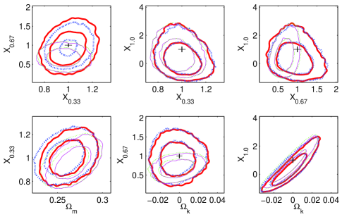
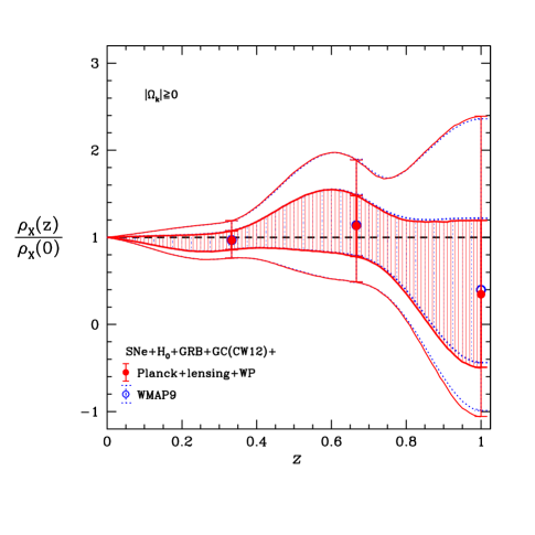
Figs.5-8 summarize our constraints on X​(z)𝑋𝑧X(z) parametrized by its value at z=1/3𝑧13z=1/3, 2/3232/3, and 1. Planck data give very similar results as WMAP9 data on X​(z)𝑋𝑧X(z), even although Planck data favor higher Ξ©msubscriptΞ©π‘š\Omega_{m}. However, note that adding Planck priors leads to a marginal inconsistency with a cosmological constant in a flat universe (see bottom right panel in Fig.6).

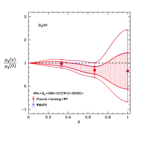
Adding BOSS data has a more significant impact: it shifts the value of X0.67subscript𝑋0.67X_{0.67} away from 1 at ∼similar-to\sim\,1.5ΟƒπœŽ\sigma (see Fig.6 and Fig.8), independent of cosmic curvature.

Refer to caption
Figure 5: The marginalized probability distributions for {X0.33,X0.67,X1.0,Ξ©m,Ξ©k,h,Ο‰b,Ξ±,Ξ²,β„³}subscript𝑋0.33subscript𝑋0.67subscript𝑋1.0subscriptΞ©π‘šsubscriptΞ©π‘˜β„Žsubscriptπœ”π‘π›Όπ›½β„³\{X_{0.33},X_{0.67},X_{1.0},\Omega_{m},\Omega_{k},h,\omega_{b},\alpha,\beta,{\cal M}\}, for SNe+H0subscript𝐻0H_{0}+GRB+GC(CW12), combined with Planck+lensing+WP (solid) and WMAP9 (dotted) data respectively.
Refer to caption
Figure 6: The joint 68% and 95% confidence contours for parameters of interest for SNe+H0subscript𝐻0H_{0}+GRB+GC(CW12), combined with Planck+lensing+WP (solid) and WMAP9 (dotted) data respectively. The thin solid and dotted contours also include GC data from BOSS.
Refer to caption
Figure 7: The 68% and 95% confidence constraints for X​(z)𝑋𝑧X(z) (cubic-splined from {X0.33,X0.67,X1.0}subscript𝑋0.33subscript𝑋0.67subscript𝑋1.0\{X_{0.33},X_{0.67},X_{1.0}\}), for SNe+H0subscript𝐻0H_{0}+GRB+GC(CW12), combined with Planck+lensing+WP (solid) and WMAP9 (dotted) data respectively.
Refer to caption
Figure 8: The 68% and 95% confidence constraints for X​(z)𝑋𝑧X(z) (cubic-splined from {X0.33,X0.67,X1.0}subscript𝑋0.33subscript𝑋0.67subscript𝑋1.0\{X_{0.33},X_{0.67},X_{1.0}\}), for SNe+H0subscript𝐻0H_{0}+GRB+GC(CW12+BOSS), combined with Planck+lensing+WP (solid) and WMAP9 (dotted) data respectively.

III.2 Constraints on a linear dark energy equation of state

We have studied the constraints on both (w0,wasubscript𝑀0subscriptπ‘€π‘Žw_{0},w_{a}) and (w0,w0.5subscript𝑀0subscript𝑀0.5w_{0},w_{0.5}), as these have different base parameters (assumed to have flat priors). In order to compare with previous work, and to display the impact of replacing WMAP9 priors with Planck+lensing+WP priors, we do not include GC data from BOSS in this comparison.

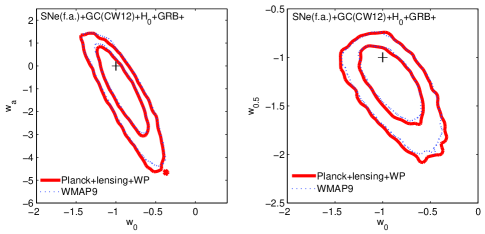
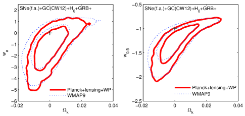
Fig.9 shows the joint 68% and 95% confidence contours for (w0,wasubscript𝑀0subscriptπ‘€π‘Žw_{0},w_{a}) (left panel) and (w0,w0.5subscript𝑀0subscript𝑀0.5w_{0},w_{0.5}) (right panel), for SNe+H0subscript𝐻0H_{0}+GRB+GC(CW12), combined with Planck+lensing+WP (solid) and WMAP9 (dotted) data respectively. Fig.10 shows the corresponding joint 68% and 95% confidence contours for (Ξ©k,wasubscriptΞ©π‘˜subscriptπ‘€π‘Ž\Omega_{k},w_{a}) (left panel) and (Ξ©k,w0.5subscriptΞ©π‘˜subscript𝑀0.5\Omega_{k},w_{0.5}) (right panel), for the same data and with the same line types. Fig.9 indicates that Planck priors do not have a significant impact on the constraints on a linear dark energy equation state; this means that the DETF FoM remains approximately the same compared to that found by Wang, Chuang, & Mukherjee (2012) using WMAP7 priors (using WMAP9 priors gives similar results as using WMAP7 priors). It is interesting to note that the right panel of Fig.10 shows that the combined data with Planck priors rule out w0.5=βˆ’1subscript𝑀0.51w_{0.5}=-1 and a flat universe at βˆΌβ€‰1.5​σsimilar-toabsent1.5𝜎\sim\,1.5\sigma. Planck data favor a small but positive Ξ©ksubscriptΞ©π‘˜\Omega_{k} (i.e., a slightly open universe).

Refer to caption
Figure 9: The joint 68% and 95% confidence contours for (w0,wasubscript𝑀0subscriptπ‘€π‘Žw_{0},w_{a}) (left panel) and (w0,w0.5subscript𝑀0subscript𝑀0.5w_{0},w_{0.5}) (right panel), for SNe+H0subscript𝐻0H_{0}+GRB+GC(CW12), combined with Planck+lensing+WP (solid) and WMAP9 (dotted) data respectively.
Refer to caption
Figure 10: The joint 68% and 95% confidence contours for (Ξ©k,wasubscriptΞ©π‘˜subscriptπ‘€π‘Ž\Omega_{k},w_{a}) (left panel) and (Ξ©k,w0.5subscriptΞ©π‘˜subscript𝑀0.5\Omega_{k},w_{0.5}) (right panel), for SNe+H0subscript𝐻0H_{0}+GRB+GC(CW12), combined with Planck+lensing+WP (solid) and WMAP9 (dotted) data respectively.

III.3 Constraints on a constant dark energy equation of state

In order to understand better the difference between the Planck+lensing+WP priors and the WMAP9 priors, we now study a constant dark energy equation of state, for the minimal combination of SNe+H0subscript𝐻0H_{0} data with the CMB priors.

Refer to caption
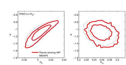
Figure 11: The joint 68% and 95% confidence contours for (Ξ©k,wsubscriptΞ©π‘˜π‘€\Omega_{k},w) (left panel) and (Ξ©m,wsubscriptΞ©π‘šπ‘€\Omega_{m},w) (right panel), for SNe+H0subscript𝐻0H_{0}, combined with Planck+lensing+WP (solid) and WMAP9 (dotted) data respectively.

Fig.11 shows the joint 68% and 95% confidence contours for (Ξ©k,wsubscriptΞ©π‘˜π‘€\Omega_{k},w) (left panel) and (Ξ©m,wsubscriptΞ©π‘šπ‘€\Omega_{m},w) (right panel), for SNe+H0subscript𝐻0H_{0}, combined with Planck+lensing+WP (solid) and WMAP9 (dotted) data respectively. Here, we see even more clearly the trend of Planck+lensing+WP priors favoring a small but postive Ξ©ksubscriptΞ©π‘˜\Omega_{k} (a slightly open universe), and a somewhat higher Ξ©msubscriptΞ©π‘š\Omega_{m}, compared to WMAP9 priors. Again, we find that adding Planck priors to other data leads to a marginal inconsistency with a cosmological constant in a flat universe.

IV Discussion and Summary

We have derived the distance priors from Planck first data release, in the form of the mean values and covariance matrix of {R,la,Ξ©b​h2,ns}𝑅subscriptπ‘™π‘ŽsubscriptΩ𝑏superscriptβ„Ž2subscript𝑛𝑠\{R,l_{a},\Omega_{b}h^{2},n_{s}\}, which give an efficient summary of Planck data in the context of dark energy constraints. As a test of the accuracy of this approach, we compare the constraints on a constant dark energy equation of state w𝑀w in a flat universe using Planck+lensing+WP data combined with SNLS SNe (no flux-averaging) in the form of MCMC chains from the Planck data archiv, with the Planck+lensing+WP data summarized by {R,la,Ξ©b​h2}𝑅subscriptπ‘™π‘ŽsubscriptΩ𝑏superscriptβ„Ž2\{R,l_{a},\Omega_{b}h^{2}\} combined with the same SN data. We find w=βˆ’1.10​(βˆ’1.18,βˆ’1.02)𝑀1.101.181.02w=-1.10\,(-1.18,-1.02) for Planck+lensing+WP data summarized by {R,la,Ξ©b​h2}𝑅subscriptπ‘™π‘ŽsubscriptΩ𝑏superscriptβ„Ž2\{R,l_{a},\Omega_{b}h^{2}\}, in excellent agreement with w=βˆ’1.12​(βˆ’1.18,βˆ’1.05)𝑀1.121.181.05w=-1.12\,(-1.18,-1.05) from the full Planck+lensing+WP data. Not surprisingly, the full CMB data give slightly tighter constraints, but the difference is not statistically significant.

We have used constraints on {R,la,Ξ©b​h2}𝑅subscriptπ‘™π‘ŽsubscriptΩ𝑏superscriptβ„Ž2\{R,l_{a},\Omega_{b}h^{2}\} from Planck data in combination with other data to probe dark energy in a conservative geometric approach. We have considered three different dark energy parametrizations: (1) Dark energy density X​(z)=ρX​(z)/ρX​(0)𝑋𝑧subscriptπœŒπ‘‹π‘§subscriptπœŒπ‘‹0X(z)=\rho_{X}(z)/\rho_{X}(0), parametrized by splining its values at z=1/3𝑧13z=1/3, 2/3, and 1.0. (2) Dark energy equation of state linear in the cosmic scale factor, wX​(z)=w0+wa​(1βˆ’a)subscript𝑀𝑋𝑧subscript𝑀0subscriptπ‘€π‘Ž1π‘Žw_{X}(z)=w_{0}+w_{a}(1-a), as well as the alternative parametrization with much less correlated parameters w0subscript𝑀0w_{0} and w0.5subscript𝑀0.5w_{0.5}, wX​(z)=w0​(3​aβˆ’2)+3​w0.5​(1βˆ’a)subscript𝑀𝑋𝑧subscript𝑀03π‘Ž23subscript𝑀0.51π‘Žw_{X}(z)=w_{0}(3a-2)+3w_{0.5}(1-a). (3) Constant dark energy equation of state wX​(z)=wsubscript𝑀𝑋𝑧𝑀w_{X}(z)=w.

In addition to CMB priors, we used SNe compiled by Conley et al. (2011) Conley11 , flux-averaged to reduce systematic errors, the Hubble constant measurement by Riess et al. (2011) Riess et al. (2011), the GRB data as summarized in Wang (2008) Wang08c , and GC data from SDSS DR7 derived by Chuang & Wang (2012) CW12 . We have chosen to use the same data as in Wang, Chuang, & Mukherjee (2012), except for the CMB priors (Planck+lensing+WP and WMAP9, versus WMAP7), in order to compare the impact of the various CMB priors. For completeness, we have added the GC data from BOSS derived by Chuang et al. (2013) Chuang et al. (2013) in constraining X​(z)𝑋𝑧X(z).

We find that when dark energy density is allowed to be a free function, current data (excluding GC data from BOSS, with either Planck+lensing+WP or WMAP priors) are fully consistent with a cosmological constant and a flat universe at 95% C.L., but deviate from a cosmological constant in a flat universe at ∼similar-to\sim\,68% C.L. (see Fig.6). The addition of BOSS data leads to a deviation from a cosmological constant at the redshift near that of the BOSS data at > 68%absentpercent68>\,68\% confidence independent of cosmic curvature (see Fig.6). In general, adding Planck+lensing+WP priors leads to a preference for a small positive Ξ©ksubscriptΞ©π‘˜\Omega_{k} (i.e., a slightly open universe) for a cosmological constant, or a flat universe with dark energy deviating from a cosmological constant, compared to adding WMAP9 priors (see Fig.6).

When dark energy equation of state is assumed to be a linear function in the cosmic scale factor a​(t)π‘Žπ‘‘a(t), the dark energy constraints depend on the base parameters used, the highly correlated {w0,wa}subscript𝑀0subscriptπ‘€π‘Ž\{w_{0},w_{a}\}, or the much less correlated {w0,w0.5}subscript𝑀0subscript𝑀0.5\{w_{0},w_{0.5}\}. The constraints on {w0,wa}subscript𝑀0subscriptπ‘€π‘Ž\{w_{0},w_{a}\} are consistent with a cosmological constant and a flat universe for both Planck+lensing+WP and WMAP9 priors, while that on {w0,w0.5}subscript𝑀0subscript𝑀0.5\{w_{0},w_{0.5}\} are marginally inconsistent with a cosmological constant in a flat universe (see Fig.9 and Fig.10) for Planck+lensing+WP priors, similar to our findings in the X​(z)𝑋𝑧X(z) case.

We find that the above trend in the Planck+lensing+WP versus WMAP9 comparison becomes more pronounced when we assume a constant dark energy equation of state. Here we only combine CMB priors with a minimal set of other data, SNe and H0subscript𝐻0H_{0}, to highlight the difference between Planck+lensing+WP and WMAP9 priors. We find that adding the Planck+lensing+WP priors to the SNe and H0subscript𝐻0H_{0} measurement leads to an inconsistency with a cosmological constant in a flat universe at > 68absent68>\,68% confidence level (see Fig.11).

To conclude, we find that Planck distance priors are significantly tighter than those from WMAP9 (see Figs.1-3). However, adding Planck distance priors does not lead to significantly improved dark energy constraints using current data, compared to adding WMAP9 distance priors. This is because Planck data appear to favor a higher matter density and lower Hubble constant Ade et al. (2013), in tension with most of the other current cosmological data sets.

In order to understand the nature of dark energy, we will need to improve our understanding of the systematic uncertainties of all data used. Future dark energy measurements from space jedi ; Cimatti09 ; euclid ; wfirst that minimize systematic uncertainties by design will enable us to make dramatic progress in our quest to shed light on dark energy.


Acknowledgments We acknowledge the use of Planck data archiv and CosmoMC. This work is supported in part by DOE grant DE-FG02-04ER41305.

References

  • Riess et al.Β  (1998) Riess, A. G, et al., 1998, Astron. J., 116, 1009
  • Perlmutter et al.Β  (1999) Perlmutter, S. et al., 1999, ApJ, 517, 565
  • (3) Copeland, E.Β J., Sami, M., Tsujikawa, S., IJMPD, 15 (2006), 1753
  • (4) Ruiz-Lapuente, P., Class. Quantum. Grav., 24 (2007), 91
  • (5) Ratra, B., Vogeley, M.Β S., arXiv:0706.1565 (2007)
  • (6) Frieman, J., Turner, M., Huterer, D., ARAA, 46, 385 (2008)
  • (7) Caldwell, R. R., & Kamionkowski, M., arXiv:0903.0866
  • (8) Uzan, J.-P., arXiv:0908.2243
  • (9) Wang, Y., Dark Energy, Wiley-VCH (2010)
  • (10) Li, M., et al., 2011, arXiv1103.5870
  • (11) Weinberg, D. H.; et al., Physics Reports, in press, arXiv:1201.2434
  • Blake & Glazebrook (2003) Blake, C.; Glazebrook, K., 2003, ApJ, 594, 665
  • Seo & Eisenstein (2003) Seo, H; Eisenstein, D J 2003, ApJ, 598, 720
  • Hu (2002) Hu, W., 2002, PRD, 66, 083515
  • Jain & Taylor (2003) Jain, B. & Taylor, A. PRL, 91, 141302 (2003)
  • Komatsu et al. (2011) Komatsu, E., et al. 2011, Astrophys.J.Suppl., 192, 18
  • Riess et al.Β  (2011) Riess, A. G, et al., 2011, ApJ, 730, 119
  • (18) Amati, L., et al. 2002, A&A, 390, 81
  • Bloom, Frail, & Kulkarni (2003) Bloom, J. S., Frail, D. A., & Kulkarni, S. R. 2003, ApJ, 594, 674
  • (20) Schaefer, B. E., 2003, ApJ, 583, L71
  • Wang (2008a) Wang, Y., Journal of Cosmology and Astroparticle Physics, 05, 021 (2008).
  • Simpson & Peacock (2010) Simpson, F., & Peacock, J.A. 2010, Phys Rev D, 81, 043512
  • Page (2003) Page, L., et al. 2003, ApJS, 148, 233
  • Wang & Mukherjee (2007) Wang, Y., & Mukherjee, P., PRD, 76, 103533 (2007)
  • (25) Li, H., et al., ApJ, 683, L1 (2008)
  • (26) Wang, Y., 2008b, Phys. Rev. D 77, 123525
  • Hu & Sugiyama (1996) Hu, W., & Sugiyama, N. 1996, ApJ, 471, 542
  • Eisenstein & Hu (1998) Eisenstein, D. & Hu, W. 1998, ApJ, 496, 605
  • Ade et al. (2013) Ade, P. A. R., et al., arXiv:1303.5076
  • Bennett et al. (2012) Bennett, C. L., et al., arXiv:1212.5225
  • Wang, Chuang, & Mukherjee (2012) Wang, Y.; Chuang, C.-H.; & Mukherjee, P., Phys. Rev. D 85, 023517 (2012)
  • (32) Chuang, C.-H.; and Wang, Y., MNRAS, 426, 226 (2012)
  • (33) Conley, A., et al., 2011, Astrophys.J.Suppl., 192, 1
  • Wang (2000) Wang, Y., ApJ 536, 531 (2000)
  • Wang & Mukherjee (2004) Wang, Y., & Mukherjee, P. 2004, ApJ, 606, 654
  • Wang (2005) Wang, Y., JCAP, 03, 005 (2005)
  • (37) Hui, L., & Greene, P.B., PRD, 73, 123526 (2006)
  • (38) Clarkson, C., et al., arXiv:1109.2484v2
  • Chuang et al. (2013) Chuang, C.H., et al., arXiv:1303.4486
  • (40) Wang, Y., 2008b, PRD, 78, 123532
  • (41) Schaefer, B. E., 2007, ApJ, 660, 16
  • (42) Butler, N.R. et al., ApJ, 2007, 671, 656
  • (43) Butler, N.R. et al., ApJ, 2009, 694, 76
  • (44) Petrosian, V.; Bouvier, A.; Ryde, F., arXiv:0909.5051
  • (45) Shahmoradi, A., & Nemiroff, R.J., MNRAS, 2011, 411, 1843
  • Wang & Garnavich (2001) Wang, Y., and Garnavich, P. 2001, ApJ, 552, 445
  • Wang & Tegmark (2004) Wang, Y., & Tegmark, M. 2004, Phys. Rev. Lett., 92, 241302
  • Wang & Freese (2006) Wang, Y., & Freese, K. 2006, Phys.Lett. B632, 449 (astro-ph/0402208)
  • Linde (1987) Linde, A. D., β€œInflation And Quantum Cosmology,” in Three hundred years of gravitation, (Eds.: Hawking, S.W. and Israel, W., Cambridge Univ. Press, 1987), 604-630.
  • (50) Wang, Y.; Kratochvil, J. M.; Linde, A.; & Shmakova, M., JCAP 0412 (2004) 006
  • Chev01 (2001) Chevallier, M., & Polarski, D. 2001, Int. J. Mod. Phys. D10, 213
  • Lewis02 (2002) Lewis, A., & Bridle, S. 2002, PRD, 66, 103511
  • (53) Crotts, A. et al., 2005, astro-ph/0507043
  • (54) Cimatti, A., et al., Experimental Astronomy, 23, 39 (2009)
  • (55) Laureijs, R.; et al., 2011, arXiv1110.3193
  • (56) Green, J.; et al., 2012, arXiv1208.4012