Abstraction and Acceleration in SMT-based Model-Checking for Array Programs

Abstract

Abstraction (in its various forms) is a powerful established technique in model-checking; still, when unbounded data-structures are concerned, it cannot always cope with divergence phenomena in a satisfactory way. Acceleration is an approach which is widely used to avoid divergence, but it has been applied mostly to integer programs. This paper addresses the problem of accelerating transition relations for unbounded arrays with the ultimate goal of avoiding divergence during reachability analysis of abstract programs. For this, we first design a format to compute accelerations in this domain; then we show how to adapt the so-called ‘monotonic abstraction’ technique to efficiently handle complex formulæ with nested quantifiers generated by the acceleration preprocessing. Notably, our technique can be easily plugged-in into abstraction/refinement loops, and strongly contributes to avoid divergence: experiments conducted with the MCMT model checker attest the effectiveness of our approach on programs with unbounded arrays, where acceleration and abstraction/refinement technologies fail if applied alone.

1 Introduction

Transitive closure is a logical construct that is far beyond first order logic: either infinite disjunctions or higher order quantifiers or, at least, fixpoints operators are required to express it. Indeed, due to the compactness of first order logic, transitive closure (even modulo the axioms of a first order theory) is first-order definable only in trivial cases. These general results do not hold if we define a theory as a class of structures $\mathcal{C}$ over a given signature. Such definition is different from the “classical” one where a theory is identified as a set of axioms. By taking a theory as a class of structures the property of compactness breaks, and it might well happen that transitive closure becomes first-order definable (the first order definition being valid just inside the class $\mathcal{C}$ - which is often reduced to a single structure).

In this paper we consider the extension of Presburger arithmetic with free unary function symbols. Inside Presburger arithmetic, various classes of relations are known to have definable acceleration (see related work section below). In our combined setting, the presence of free function symbols introduces a novel feature that, for instance, limits decidability to controlled extensions of the quantifier-free fragment [15, 22]. In this paper we show that in such theory some classes of relations admit a definable acceleration.

The theoretical problem of studying the definability of accelerated relations has an important application in program verification. The theory we focus on is widely adopted to represent programs handling arrays, where free functions model arrays of integers. In this application domain, the accelerated counterpart of relations encoding systems evolution (e.g., loops in programs) allows to compute ‘in one shot’ the reachable set of states after an arbitrary but finite number of execution steps. This has the great advantage of keeping under control sources of (possible) divergence arising in the reachability analysis.

The contributions of the paper are many-fold. First, we show that inside the combined theory of Presburger arithmetic augmented with free function symbols, the acceleration of some classes of relations – corresponding, in our application domain, to relations involving arrays and counters – can be expressed in first order language. This result comes at a price of allowing nested quantifiers. Such nested quantification can be problematic in practical applications. To address this complication, as a second contribution of the paper, we show how to take care of the quantifiers added by the accelerating procedure: the idea is to import in this setting the so-called monotonic abstraction technique [2, 1]. Such technique has been reinterpreted and analyzed in a declarative context in [5]: from a logical point of view, it amounts to a restricted form of instantiation for universal quantifiers. Third, we show that the ability to compute accelerated relations is greatly beneficial in program verification. In particular, one of the biggest problems in verifying safety properties of array programs is designing procedures for the synthesis of relevant quantified predicates. In typical sequential programs (like those illustrated in Figure1), the guarded assignments used to model the program instructions are ground and, as a consequence, the formulae representing backward reachable states are ground too. However, the invariants required to certify the safety of such programs contain quantifiers. Our acceleration procedure is able to supply the required quantified predicates. Our experimentation attests that abstraction/refinement-based strategies widely used in verification benefit from accelerated transitions. In programs with nested loops, as the allDiff procedure of Figure1 for example, the ability to accelerate the inner loop simplifies the structure of the problem, allowing abstraction to converge during verification of the entire program. For such programs, abstraction/refinement or acceleration approaches taken in isolation are not sufficient, reachability analysis converges only if they are combined together.

Related Work.  To the best of our knowledge, the only work addressing the problem of accelerating relations involving arrays is [12]. Such approach seems to be unable to handle properties of common interest with more than one quantified variable (e.g., “sortedness”) and is limited to programs without nested loops. Our technique is not affected by such limitations and can successfully handle examples outside the scope of [12].

Inside Presburger arithmetic, various classes of relations are known to have definable acceleration: these include relations that can be formalized as difference bounds constraints [19, 14], octagons [11] and finite monoid affine transformations [20] (paper [13] presents a general approach covering all these domains). Acceleration for relations over Presburger arithmetic has been also plugged into abstraction/refinement loop for verifying integer programs [16, 26].

We recall that acceleration has also been applied proficiently in the analysis of real time systems (e.g., [25, 8]), to compactly represent the iterated execution of cyclic actions (e.g., polling-based systems) and address fragmentation problems.

Our work can be proficiently combined with SMT-based techniques for the verification of programs, as it helps helps avoiding the reachability analysis divergence when it comes to abstraction of programs with arrays of unknown length. Since the technique mostly operates at pre-processing level (we add to the system accelerated transitions by collapsing branches of loops handling arrays), we believe that our technique is compatible with most approaches proposed in array-based software model checking. We summarize some of these approaches below, without pretending of being exhaustive.

The vast majority of software model-checkers implement abstraction-refinement algorithms (e.g., [24, 18, 6]). Lazy Abstraction with Interpolants [30] is one of the most effective frameworks for unbounded reachability analysis of programs. It relies on the availability of interpolation procedures (nowadays efficiently embedded in SMT-Solvers [17]) to generate new predicates as (quantifier-free) interpolants for refining infeasible counterexamples.

$${\sf function}\leavevmode\nobreak\ {\tt allDiff}\leavevmode\nobreak\ (\leavevmode\nobreak\ {\sf int}\leavevmode\nobreak\ {\tt a}[{\tt N}]\leavevmode\nobreak\ ):\leavevmode\nobreak\$$

$$1\leavevmode\nobreak\ \leavevmode\nobreak\ {\tt r}={\sf true};$$

$$2\leavevmode\nobreak\ \leavevmode\nobreak\ {\sf for}\leavevmode\nobreak\ ({\tt i}=1;\leavevmode\nobreak\ {\tt i}<{\tt N}\wedge{\tt r};{\tt i}\text{+}\text{+})\leavevmode\nobreak\$$

$$3\leavevmode\nobreak\ \leavevmode\nobreak\ \leavevmode\nobreak\ \leavevmode\nobreak\ \leavevmode\nobreak\ {\sf for}\leavevmode\nobreak\ ({\tt j}={\tt i}\text{-}1;{\tt j}\geq 0\wedge{\tt r};{\tt j}\text{-}\text{-})\leavevmode\nobreak\$$

$$4\leavevmode\nobreak\ \leavevmode\nobreak\ \leavevmode\nobreak\ \leavevmode\nobreak\ \leavevmode\nobreak\ \leavevmode\nobreak\ \leavevmode\nobreak\ {\sf if}\leavevmode\nobreak\ ({\tt a}[{\tt i}]={\tt a}[{\tt j}])\leavevmode\nobreak\ {\tt r}={\sf false};$$

$$5\leavevmode\nobreak\ \leavevmode\nobreak\ {\sf assert}\leavevmode\nobreak\ \left({\tt r}\rightarrow\left(\begin{aligned} &\forall x,y(0\leq x<y<{\tt N})\\ &\leavevmode\nobreak\ \leavevmode\nobreak\ \leavevmode\nobreak\ \leavevmode\nobreak\ \leavevmode\nobreak\ \rightarrow({\tt a}[x]\neq{\tt a}[y])\end{aligned}\right)\right)$$

(a)

$${\sf function}\leavevmode\nobreak\ {\tt Reverse}\leavevmode\nobreak\ (\leavevmode\nobreak\ {\sf int}\leavevmode\nobreak\ {\tt I}[{\tt N}+1];\leavevmode\nobreak\ {\sf int}\leavevmode\nobreak\ {\tt O}[{\tt N}+1];\leavevmode\nobreak\ {\sf int}\leavevmode\nobreak\ {\tt c}\leavevmode\nobreak\ ):$$

$$1\leavevmode\nobreak\ \leavevmode\nobreak\ {\tt c}=0;$$

$$2\leavevmode\nobreak\ \leavevmode\nobreak\ {\sf while}\leavevmode\nobreak\ ({\tt c}\neq N+1)\leavevmode\nobreak\ \{{\tt O}[{\tt c}]={\tt I}[N-{\tt c}];{\tt c\!+\!+};\}$$

$$3\leavevmode\nobreak\ \leavevmode\nobreak\ {\sf assert}\leavevmode\nobreak\ \left(\begin{aligned} &\forall x\geq 0,y\geq 0\\ &\leavevmode\nobreak\ \leavevmode\nobreak\ \leavevmode\nobreak\ (x+y={\tt N}\to{\tt I}[x]={\tt O}[y]\leavevmode\nobreak\ )\leavevmode\nobreak\ \end{aligned}\right)$$

(b)

Figure 1: Motivating examples.

For programs with arrays of unknown length the classical interpolation-based lazy abstraction works only if there is a support to handle quantified predicates [3] (the approach of [3] is the basis of our experiments below). Effectiveness and performances of abstraction/refinement approaches strongly depend on their ability in generating the “right” predicates to stop divergence of verification procedures. In case of programs with arrays, this quest can rely on ghost variables [21] retrieved from the post-conditions, on the backward propagation of post-conditions along spurious counterexamples [33] or can be constraint-based [34, 9]. Recently, constraint-based techniques have been significantly extended to the generation of loop invariants outside the array property fragment [29]. This solution exploits recent advantages in SMT-Solving, namely those devoted to finding solutions of constraints over non-linear integer arithmetic [10]. Other ways to generate predicates are by means of saturation-based theorem provers [28, 31] or interpolation procedures [27, 3].

All the aforementioned techniques suffer from a certain degree of randomness due to the fact that detecting the “right” predicate is an undecidable problem. For example, predicate abstraction approaches (i.e., [3, 4, 33]) fail verifying the procedures in Figure1, which are commonly considered to be challenging for verifiers because they cause divergence. Acceleration, on the other side, provides a precise and systematic way for addressing the verification of programs. Its combination, as a preprocessing procedure, with standard abstraction-refinement techniques allows to successfully solve challenging problems like the ones in Figure1.

The paper is structured as follows: Section 2 recalls the background notions about Presburger arithmetic and extensions. In order to identify the classes of relations whose acceleration we want to study, we are guided by software model checking applications. To this end, we provide in Section 3 classification of the guarded assignments we are interested in. Section 4 demonstrates the practical application of the theoretical results. In particular, it presents a backward reachability procedure and shows how to plug acceleration with monotonic abstraction in it. The details of the theoretical results are presented later. The main definability result for accelerations is in Section 6, while Section 5 introduces the abstract notion of an iterator. Section 7 discusses our experiments and Section 8 concludes the paper.

2 Preliminaries

We work in Presburger arithmetic enriched with free function symbols and with definable function symbols (see below); when we speak about validity or satisfiability of a formula, we mean satisfiability and validity in all structures having the standard structure of natural numbers as reduct. Thus, satisfiability and validity are decidable if we limit to quantifier-free formulæ (by adapting Nelson-Oppen combination results [32, 35]), but may become undecidable otherwise (because of the presence of free function symbols).

We use $x,y,z,\dots$ or $i,j,k,\dots$ for variables; $t,u,\dots$ for terms, $c,d,\dots$ for free constants, $a,b,\dots$ for free function symbols, $\phi,\psi,\dots$ for quantifier-free formulæ. Bold letters are used for tuples and $|-|$ indicates tuples length; hence for instance ${\bf u}$ indicates a tuple of terms like $u_{1},\dots,u_{m}$, where ${m=|{\bf u}|}$ (these tuples may contain repetitions). For variables, we use underline letters $\underline{x},\underline{y},\dots,\underline{i},\underline{j},\dots$ to indicates tuples without repetitions. Vector notation can also be used for equalities: if ${\bf u}=u_{1},\dots,u_{n}$ and ${\bf v}=v_{1},\dots,v_{n}$, we may use ${\bf u}={\bf v}$ to mean the formula $\bigwedge_{i=1}^{n}u_{i}=v_{i}$.

If we write $t(x_{1},\dots,x_{n}),{\bf u}(x_{1},\dots,x_{n}),\phi(x_{1},\dots,x_{n})$ (or $t(\underline{x}),{\bf u}(\underline{x}),\phi(\underline{x}),\dots$, in case $\underline{x}=x_{1},\dots,x_{n}$), we mean that the term $t$, the tuple of terms ${\bf u}$, the quantifier-free formula $\phi$ contain variables only from the tuple $x_{1},\dots,x_{n}$. Similarly, we may use $t({\bf a},{\bf c},\underline{x}),\phi({\bf a},{\bf c},\underline{x}),\dots$ to mean both that the term $t$ or the quantifier-free formula $\phi$ have free variables included in $\underline{x}$ and that the free function, free constants symbols occurring in them are among ${\bf a},{\bf c}$. Notations like $t({\bf u}/\underline{x}),\phi({\bf u}/\underline{x}),\dots$ or $t(u_{1}/x_{1},\dots,u_{n}/x_{n}),\phi(u_{1}/x_{1},\dots,u_{n}/x_{n}),\dots$ - or occasionally just $t({\bf u}),\phi({\bf u}),\dots$ if confusion does not arise - are used for simultaneous substitutions within terms and formulæ. For a given natural number $n$, we use the standard abbreviations $\bar{n}$ and $n*y$ to denote the numeral of $n$ (i.e. the term $s^{n}(0)$, where $s$ is the successor function) and the sum of $n$ addends all equal to $y$, respectively. If confusion does not arise, we may write just $n$ for $\bar{n}$.

By a definable function symbol, we mean the following. Take a quantifier-free formula $\phi(\underline{j},y)$ such that $\forall\underline{j}\exists!y\phi(\underline{j},y)$ is valid ($\exists!y$ stands for ‘there is a unique $y$ such that …’). Then a definable function symbol $F$ (defined by $\phi$) is a fresh function symbol, matching the length of $\underline{j}$ as arity, which is constrained to be interpreted in such a way that the formula $\forall y.F(\underline{j})=y\leftrightarrow\phi(\underline{j},y)$ is true. The addition of definable function symbols does not affect decidability of quantifier-free formulæ and can be used for various purposes, for instance in order to express directly case-defined functions, array updates, etc. For instance, if $a$ is a unary free function symbol, the term $wr(a,i,x)$ (expressing the update of the array $a$ at position $i$ by over-writing $x$) is a definable function; formally, we have $\underline{j}:=i,x,j$ and $\phi(\underline{j},y)$ is given by $(j=i\wedge y=x)\vee(j\neq i\wedge y=a(j))$. This formula $\phi(\underline{j},y)$ (and similar ones) can be abbreviated like

$$y\leavevmode\nobreak\ =\leavevmode\nobreak\ (\mathtt{if}\leavevmode\nobreak\ j=i\leavevmode\nobreak\ \mathtt{then}\leavevmode\nobreak\ x\leavevmode\nobreak\ \mathtt{else}\leavevmode\nobreak\ a(j))\vspace{-0.15cm}$$

to improve readability. Another useful definable function is integer division by a fixed natural number $n$: to show that integer division by $n$ is definable, recall that in Presburger arithmetic we have that $\forall x\leavevmode\nobreak\ \exists!y\leavevmode\nobreak\ \bigvee_{r=0}^{n-1}(x=n*y+r)$ is valid.

3 Programs representation

As a first step towards our main definability result, we provide a classification of the relations we are interested in. Such relations are guarded assignments required to model programs handling arrays of unknown length.

In our framework a program $\mathcal{P}$ is represented by a tuple $({\bf v},l_{I},l_{E},T)$; the tuple ${\bf v}:={\bf a},{\bf c},pc$ models system variables; formally, we have that

-

the tuple ${\bf a}=a_{1},\dots,a_{s}$ contains free unary function symbols, i.e., the arrays manipulated by the program;

-

the tuple ${\bf c}=c_{1},\dots,c_{t}$ contains free constants, i.e., the integer data manipulated by the program;

-

the additional free constant $pc$ (called program counter) is constrained to range over a finite set $L=\{l_{1},...,l_{n}\}$ of program locations over which we distinguish the initial and error locations denoted by $l_{I}$ and $l_{E}$, respectively.

$T$ is a set of finitely many formulæ $\{\tau_{1}({\bf v},{\bf v}^{\prime}),\dots,\tau_{r}({\bf v},{\bf v}^{\prime})\}$ called transition formulæ representing the program’s body (here ${\bf v}^{\prime}$ are renamed copies of the ${\bf v}$ representing the next-state variables). $\mathcal{P}=({\bf v},l_{I},l_{E},T)$ is safe iff there is no satisfiable formula like

$$(pc^{0}=l_{I})\wedge\tau_{i_{1}}({\bf v}^{0},{\bf v}^{1})\wedge\cdots\wedge\tau_{i_{N}}({\bf v}^{N-1},{\bf v}^{N})\wedge(pc^{N}=l_{E})$$

where ${\bf v}^{0},\dots,{\bf v}^{N}$ are renamed copies of the ${\bf v}$ and each $\tau_{i_{h}}$ belongs to $T$.

Sentences denoting sets of states reachable by $\mathcal{P}$ can be:

-

ground sentences, i.e., sentences of the kind $\phi({\bf c},{\bf a},pc)$;

-

$\Sigma^{0}_{1}$-sentences, i.e., sentences of the form $\exists\underline{i}.\;\phi(\underline{i},{\bf a},{\bf c},pc)$;

-

$\Sigma^{0}_{2}$-sentences, i.e., sentences of the form $\exists\underline{i}\,\forall\underline{j}.\;\phi(\underline{i},\underline{j},{\bf a},{\bf c},pc)$.

We remark that in our context satisfiability can be fully decided only for ground sentences and $\Sigma^{0}_{1}$-sentences (by Skolemization, as a consequence of the general combination results [32, 35]), while only subclasses of $\Sigma^{0}_{2}$-sentences enjoy a decision procedure [15, 22]. Transition formulæ can also be classified in three groups:

-

ground assignments, i.e., transitions of the form

$$pc=l\leavevmode\nobreak\ \wedge\leavevmode\nobreak\ \phi_{L}({\bf c},{\bf a})\leavevmode\nobreak\ \wedge\leavevmode\nobreak\ pc^{\prime}=l^{\prime}\leavevmode\nobreak\ \wedge\leavevmode\nobreak\ {\bf a}^{\prime}=\lambda j.\;G({\bf c},{\bf a},j)\leavevmode\nobreak\ \wedge\leavevmode\nobreak\ {\bf c}^{\prime}=H({\bf c},{\bf a})$$ (1)

-

$\Sigma^{0}_{1}$-assignments, i.e., transitions of the form

$$\exists\underline{k}\;\left(\begin{split}pc=l\leavevmode\nobreak\ \wedge\leavevmode\nobreak\ \phi_{L}({\bf c},{\bf a},\underline{k})\leavevmode\nobreak\ \wedge\leavevmode\nobreak\ pc^{\prime}=l^{\prime}\leavevmode\nobreak\ \wedge\leavevmode\nobreak\ \leavevmode\nobreak\ \leavevmode\nobreak\ \leavevmode\nobreak\ \leavevmode\nobreak\ \\ {\bf a}^{\prime}=\lambda j.\;G({\bf c},{\bf a},\underline{k},j)\leavevmode\nobreak\ \wedge\leavevmode\nobreak\ {\bf c}^{\prime}=H({\bf c},{\bf a},\underline{k})\end{split}\right)$$ (2)

-

$\Sigma^{0}_{2}$-assignments, i.e., transitions of the form

$$\exists\underline{k}\;\left(\begin{split}pc=l\leavevmode\nobreak\ \wedge\leavevmode\nobreak\ \phi_{L}({\bf c},{\bf a},\underline{k})\leavevmode\nobreak\ \wedge\leavevmode\nobreak\ \forall\underline{j}\leavevmode\nobreak\ \psi_{U}({\bf c},{\bf a},\underline{k},\underline{j})\leavevmode\nobreak\ \wedge\leavevmode\nobreak\ \leavevmode\nobreak\ \leavevmode\nobreak\ \leavevmode\nobreak\ \leavevmode\nobreak\ \leavevmode\nobreak\ \\ pc^{\prime}=l^{\prime}\leavevmode\nobreak\ \wedge\leavevmode\nobreak\ {\bf a}^{\prime}=\lambda j.\;G({\bf c},{\bf a},\underline{k},j)\wedge\leavevmode\nobreak\ {\bf c}^{\prime}=H({\bf c},{\bf a},\underline{k})\end{split}\right)$$ (3)

where $G=G_{1},\dots,G_{s}$, $H=H_{1},\dots,H_{t}$ are tuples of definable functions (vectors of equations like ${\bf a}^{\prime}=\lambda j.\;G({\bf c},{\bf a},\underline{k}j)$ can be replaced by the corresponding first order sentences $\forall j.\leavevmode\nobreak\ \bigwedge_{h=1}^{s}a_{h}^{\prime}(j)=G_{h}({\bf c},{\bf a},\underline{k},j)$).

The composition $\tau_{1}\circ\tau_{2}$ of two transitions $\tau_{1}({\bf v},{\bf v}^{\prime})$ and $\tau_{2}({\bf v},{\bf v}^{\prime})$ is expressed by the formula $\exists{\bf v}_{1}(\tau_{1}({\bf v},{\bf v}_{1})\wedge\tau_{2}({\bf v}_{1},{\bf v}^{\prime}))$ (notice that composition may result in an inconsistent formula, e.g., in case of location mismatch). The preimage $Pre(\tau,K)$ of the set of states satisfying the formula $K({\bf v})$ along the transition $\tau({\bf v},{\bf v}^{\prime})$ is the set of states satisfying the formula $\exists{\bf v}^{\prime}(\tau({\bf v},{\bf v}^{\prime})\wedge K({\bf v}^{\prime}))$. The following proposition is immediate by straightforward syntactic manipulations:

Proposition 3.1.

Let $\tau,\tau_{1},\tau_{2}$ be transition formulæ and let $K({\bf v})$ be a formula. We have that: (i) if $\tau_{1},\tau_{2},\tau,K$ are ground, then $\tau_{1}\circ\tau_{2}$ is a ground assignment and $Pre(\tau,K)$ is a ground formula; (ii) if $\tau_{1},\tau_{2},\tau,K$ are $\Sigma^{0}_{1}$, then $\tau_{1}\circ\tau_{2}$ is a $\Sigma^{0}_{1}$-assignment and $Pre(\tau,K)$ is a $\Sigma^{0}_{1}$-sentence; (iii) if $\tau_{1},\tau_{2},\tau,K$ are $\Sigma^{0}_{2}$, then $\tau_{1}\circ\tau_{2}$ is a $\Sigma^{0}_{2}$-assignment and $Pre(\tau,K)$ is a $\Sigma^{0}_{2}$-sentence.

4 Backward search and acceleration

This section demonstrates the practical applicability of the theoretical results of the paper in program verification. In particular, it presents the application of the accelerated transitions during reachability analysis for guarded-assignments representing programs handling arrays. For readability, we first present a basic reachability procedure. We subsequently analyze the divergence problems and show how acceleration can be applied to solve them. Acceleration application is not straightforward, though. The presence of accelerated transitions might generate undesirable $\Sigma^{0}_{2}$-sentences. The solution we propose is to over-approximate such sentences by adopting a selective instantiation schema, known in literature as monotonic abstraction. An enhanced reachability procedure integrating acceleration and monotonic abstraction concludes the Section.

The methodology we exploit to check safety of a program $\mathcal{P}=({\bf v},l_{I},l_{E},T)$ is backward search: we successively explore, through symbolic representation, all states leading to the error location $l_{E}$ in one step, then in two steps, in three steps, etc. until either we find a fixpoint or until we reach $l_{I}$. To do this properly, it is convenient to build a tree: the tree has arcs labeled by transitions and nodes labeled by formulæ over ${\bf v}$. Leaves of the tree might be marked ‘checked’, ‘unchecked’ or ‘covered’. The tree is built according to the following non-deterministic rules.

Backward Search

Initialization: a single node tree labeled by $pc=l_{E}$ and is marked ‘unchecked’.

Check: pick an unchecked leaf $L$ labeled with $K$. If $K\wedge pc=l_{I}$ is satisfiable (‘safety test’), exit and return unsafe. If it is not satisfiable, check whether there is a set $S$ of uncovered nodes such that (i) $L\not\in S$ and (ii) $K$ is inconsistent with the conjunction of the negations of the formulæ labeling the nodes in $S$ (‘fixpoint check’). If it is so, mark $L$ as ‘covered’ (by $S$). Otherwise, mark $L$ as ‘checked’.

Expansion: pick a checked leaf $L$ labeled with $K$. For each transition $\tau_{i}\in T$, add a new leaf below $L$ labeled with $Pre(\tau_{i},L)$ and marked as ‘unchecked’. The arc between $L$ and the new leaf is labeled with $\tau_{i}$.

Safety Exit: if all leaves are covered, exit and return safe.

The algorithm may not terminate (this is unavoidable by well-known undecidability results). Its correctness depends on the possibility of discharging safety tests with complete algorithms. By Proposition 3.1, if transitions are ground- or $\Sigma^{0}_{1}$-assignments, completeness of safety tests arising during the backward reachability procedure is guaranteed by the fact that satisfiability of $\Sigma^{0}_{1}$-formulæ is decidable. For fixpoint tests, sound but incomplete algorithms may compromise termination, but not correctness of the answer; hence for fixpoint tests, we can adopt incomplete pragmatic algorithms (e.g. if in fixpoint tests we need to test satisfiability of $\Sigma^{0}_{2}$-sentences, the obvious strategy is to Skolemize existentially quantified variables and to instantiate the universally quantified ones over sets of terms chosen according to suitable heuristics). To sum up, we have:

Proposition 4.1.

The above Backward Search procedure is partially correct for programs whose transitions are $\Sigma^{0}_{1}$-assignments, i.e., when the procedure terminates it gives a correct information about the safety of the input program.

Divergence phenomena are usually not due to incomplete algorithms for fixpoint tests (in fact, divergence persists even in cases where fixpoint tests are precise).

Example 4.1.

Consider a running example in Figure 1(b): it reverses the content of the array ${\tt I}$ into ${\tt O}$. In our formalism, it is represented by the following transitions:

$$\tau_{1}\equiv\leavevmode\nobreak\ {\tt pc}=1\wedge{\tt pc}^{\prime}=2\wedge{\tt c}^{\prime}=0$$

$$\tau_{2}\equiv\leavevmode\nobreak\ {\tt pc}=2\wedge{\tt c}\neq N+1\wedge{\tt c}^{\prime}={\tt c}+1\wedge O^{\prime}=wr(O,{\tt c},I(N-{\tt c}))$$

$$\tau_{3}\equiv\leavevmode\nobreak\ {\tt pc}=2\wedge{\tt c}=N+1\wedge{\tt pc}^{\prime}=3$$

$$\tau_{4}\equiv\leavevmode\nobreak\ {\tt pc}=3\wedge\exists z_{1}\geq 0,z_{2}\geq 0\leavevmode\nobreak\ (z_{1}+z_{2}=N\wedge I(z_{1})\neq O(z_{2})\leavevmode\nobreak\ )\wedge{\tt pc}^{\prime}=4.$$

Notice that $\tau_{1}-\tau_{3}$ all are ground assignments; only $\tau_{4}$ (that translates the error condition) is a $\Sigma^{0}_{1}$-assignment. If we apply our tree generation procedure, we get an infinite branch, whose nodes - after routine simplifications - are labeled as follows

$$\cdots$$

$$(K_{i}) \leavevmode\nobreak\ \leavevmode\nobreak\ {\tt pc}=2\wedge\exists z_{1},z_{2}\;\psi(z_{1},z_{2})\wedge{\tt c}=N-i\wedge z_{2}\neq N\wedge\cdots\wedge z_{2}\neq N-i$$

$$\cdots$$

where $\psi(z_{1},z_{2})$ stands for $z_{1}\geq 0\wedge z_{2}\geq 0\wedge z_{1}+z_{2}=N\wedge I(z_{1})\neq O(z_{2})$. ∎

As demonstrated by the above example, a divergence source comes from the fact that we are unable to represent in one shot the effect of executing finitely many times a given sequence of transitions. Acceleration can solve this problem.

Definition 4.1.

The $n$-th composition of a transition $\tau({\bf v},{\bf v}^{\prime})$ with itself is recursively defined by $\tau^{1}:=\tau$ and $\tau^{n+1}:=\tau\circ\tau^{n}$. The acceleration $\tau^{+}$ of $\tau$ is $\bigvee_{n\geq 1}\tau^{n}$.

In general, acceleration requires a logic supporting infinite disjunctions. Notable exceptions are witnessed by Theorem 6.1. For now we focus on examples where accelerations yield $\Sigma^{0}_{2}$-assignments starting from ground assignments.

Example 4.2.

Recall transition $\tau_{2}$ from the running example.

$$\tau_{2}\equiv\leavevmode\nobreak\ {\tt pc}=2\wedge{\tt c}\neq N+1\wedge pc^{\prime}=2\wedge{\tt c}^{\prime}={\tt c}+1\wedge I^{\prime}=I\wedge O^{\prime}=wr(O,{\tt c},I(N-{\tt c}))$$

(here we displayed identical updates for completeness). Notice that the variable ${\tt pc}$ is left unchanged in this transition (this is essential, otherwise the acceleration gives an inconsistent transition that can never fire). If we accelerate it, we get the $\Sigma^{0}_{2}$-assignment

$$\exists n>0\leavevmode\nobreak\ \left(\begin{split}{\tt pc}=2\leavevmode\nobreak\ \wedge\leavevmode\nobreak\ \forall j\leavevmode\nobreak\ ({\tt c}\leq j<{\tt c}+n\to j\neq N+1)\leavevmode\nobreak\ \wedge\leavevmode\nobreak\ {\tt c}^{\prime}={\tt c}+n\leavevmode\nobreak\ \wedge\leavevmode\nobreak\ \leavevmode\nobreak\ \leavevmode\nobreak\ \leavevmode\nobreak\ \\ \wedge\leavevmode\nobreak\ {\tt pc}^{\prime}=2\leavevmode\nobreak\ \wedge\leavevmode\nobreak\ O^{\prime}=\lambda j\leavevmode\nobreak\ ({\tt if}\leavevmode\nobreak\ {\tt c}\leq j<{\tt c}+n\leavevmode\nobreak\ {\tt then}\leavevmode\nobreak\ I(N\!-\!j)\leavevmode\nobreak\ {\tt else}\leavevmode\nobreak\ O(j))\end{split}\right)$$ (4)

∎

In presence of these accelerated $\Sigma^{0}_{2}$-assignments, Backward Search can produce problematic $\Sigma^{0}_{2}$-sentences (see Proposition 3.1 above) which cannot be handled precisely by existing solvers. As a solution to this problem we propose applying to such sentences a suitable abstraction, namely monotonic abstraction.

Definition 4.2.

Let $\psi:\equiv\exists\underline{i}\,\forall\underline{j}.\;\phi(\underline{i},\underline{j},{\bf a},{\bf c},pc)$ be a $\Sigma^{0}_{2}$-sentences and let $\mathcal{S}$ be a finite set of terms of the kind $t(\underline{i},{\bf v})$. The monotonic $\mathcal{S}$-approximation of $\psi$ is the $\Sigma^{0}_{1}$-sentence

$$\exists\underline{i}\;\bigwedge_{\sigma:\underline{j}\to\mathcal{S}}\phi(\underline{i},\underline{j}\sigma/\underline{j},{\bf a},{\bf c},pc)$$ (5)

(here $\underline{j}\sigma$, if $\underline{j}=j_{1},\dots,j_{n}$, is the tuple of terms $\sigma(j_{1}),\dots,\sigma(j_{n})$).

By Definition 4.2, universally quantified variables are eliminated through instantiation; the larger the set $\mathcal{S}$ is, the better approximation you get. In practice, the natural choices for $\mathcal{S}$ are $\underline{i}$ or the set of terms of the kind $t(\underline{i},{\bf v})$ occurring in $\psi$ (we adopted the former choice in our implementation). As a result of replacing $\Sigma^{0}_{2}$-sentences by their monotonic approximation, spurious unsafe traces might occur. However, those can be disregarded if accelerated transitions contribute to their generation. This is because if $\mathcal{P}$ is unsafe, then unsafety can be discovered without appealing to accelerated transitions.

To integrate monotonic abstraction, the above Backward Search procedure is modified as follows. In a Preprocessing step, we add some accelerated transitions of the kind $(\tau_{1}\circ\cdots\circ\tau_{n})^{+}$ to $T$. These transitions can be found by inspecting cycles in the control flow graph of the program and accelerating them following the procedure described in Sections 5, 6. The natural cycles to inspect are those corresponding to loop branches in the source code. It should be noticed, however, that identifying the good cycles to accelerate is subject to specific heuristics that deserve separate investigation in case the program has infinitely many cycles. (choosing cycles from branches of innermost loops is the simplest example of such heuristics and the one we implemented).

After this extra preprocessing step, the remaining instructions are left unchanged, with the exception of Check that is modified as follows:

Check’: pick an unchecked leaf $L$ labeled by a formula $K$. If $K$ is a $\Sigma^{0}_{2}$-sentence, choose a suitable $\mathcal{S}$ and replace $K$ by its monotonic $\mathcal{S}$-abstraction $K^{\prime}$. If $K^{\prime}\wedge pc=l_{I}$ is inconsistent, mark $L$ as ‘covered’ or ‘checked’ according to the outcome of the fixpoint check, as was done in the original Check. If $K^{\prime}\wedge pc=l_{I}$ is satisfiable, analyze the path from the root to $L$. If no accelerated transition $\tau^{+}$ is found in it return unsafe, otherwise remove the sub-tree $D$ from the target of $\tau^{+}$ to the leaves. Each node $N$ covered by a node in $D$ will be flagged as ‘unchecked’ (to make it eligible in future for the Expansion instruction).

The new procedure will be referred as Backward Search’. It is quite straightforward to see that Proposition 4.1 still applies to the modified algorithm. Notice that, although termination cannot be ensured (given well-known undecidability results), spurious traces containing approximated accelerated transitions cannot be produced again and again: when the sub-tree $D$ from the target node $v$ of $\tau^{+}$ is removed by Check’, the node $v$ is not a leaf (the arcs labeled by the transitions $\tau$ are still there), hence it cannot be expanded anymore according to the Expansion instruction.

Example 4.3.

Let again consider our running example and demonstrate how acceleration and monotonic abstraction work. In the preprocessing step, we add the accelerated transition $\tau_{2}^{+}$ given by (4) to the transitions we already have. After having computed $(K^{\prime})\equiv Pre(\tau_{4},K),(K^{\prime\prime})\equiv Pre(\tau_{3},K^{\prime})$, we compute $(\tilde{K})\equiv Pre(\tau_{2}^{+},K^{\prime\prime})$ and get

$$\exists n>0\,\exists z_{1},z_{2}\,\left(\begin{split}{\tt pc}=2\leavevmode\nobreak\ \wedge\leavevmode\nobreak\ \forall j\leavevmode\nobreak\ ({\tt c}\leq j<{\tt c}\!+\!n\to j\neq N\!+\!1)\leavevmode\nobreak\ \wedge\leavevmode\nobreak\ \leavevmode\nobreak\ \leavevmode\nobreak\ \leavevmode\nobreak\ \leavevmode\nobreak\ \leavevmode\nobreak\ \leavevmode\nobreak\ \leavevmode\nobreak\ \\ \wedge\leavevmode\nobreak\ {\tt c}\!+\!n=N\!+\!1\leavevmode\nobreak\ \wedge z_{1}\geq 0\leavevmode\nobreak\ \wedge\leavevmode\nobreak\ z_{2}\geq 0\leavevmode\nobreak\ \wedge z_{1}+z_{2}=N\leavevmode\nobreak\ \wedge\leavevmode\nobreak\ \\ \wedge\leavevmode\nobreak\ I(z_{1})\neq\lambda j\leavevmode\nobreak\ ({\tt if}\leavevmode\nobreak\ {\tt c}\leq j<{\tt c}+n\leavevmode\nobreak\ {\tt then}\leavevmode\nobreak\ I(N\!-\!j)\leavevmode\nobreak\ {\tt else}\leavevmode\nobreak\ O(j))(z_{2})\end{split}\right)$$

We approximate using the set of terms $\mathcal{S}=\{z_{1},z_{2},n\}$. After simplifications we get

$$\exists z_{1},z_{2}\,({\tt pc}=2\leavevmode\nobreak\ \wedge\leavevmode\nobreak\ {\tt c}\leq N\leavevmode\nobreak\ \wedge z_{1}\geq 0\leavevmode\nobreak\ \wedge\leavevmode\nobreak\ z_{2}\geq 0\leavevmode\nobreak\ \wedge\leavevmode\nobreak\ z_{1}+z_{2}=N\leavevmode\nobreak\ \wedge\leavevmode\nobreak\ O(z_{2})\neq I(z_{1})\leavevmode\nobreak\ \wedge\leavevmode\nobreak\ {\tt c}>z_{2})\vspace{-0.1cm}$$

Generating this formula is enough to stop divergence. ∎

Notice that in the computations of the above example we eventually succeeded in eliminating the extra quantifier $\exists n$ introduced by the accelerated transition. This is not always possible: sometimes in fact, to get the good invariant one needs more quantified variables than those occurring in the annotated program and accelerated transitions might be the way of getting such additional quantified variables. As an example of this phenomenon, consider the init+test program included in our benchmark suite of Section 7 below.

5 Iterators

This Section introduces iterators and selectors, two main ingredients used to supply a useful format to compute accelerated transitions. Iterators are meant to formalize the notion of a counter scanning the indexes of an array: the most simple iterators are increments and decrements, but one may also build more complex ones for different scans, like in binary search. We give their formal definition and then we supply some examples. We need to handle tuples of terms because we want to consider the case in which we deal with different arrays with possibly different scanning variables. Given a $m$-tuple of terms

$${\bf u}(\underline{x})\leavevmode\nobreak\ :=\leavevmode\nobreak\ u_{1}(x_{1},\dots,x_{m}),\dots,u_{m}(x_{1},\dots,x_{m})$$ (6)

containing the $m$ variables $\underline{x}=x_{1},\dots,x_{m}$, we indicate with ${\bf u}^{n}$ the term expressing the $n$-times composition of (the function denoted by) ${\bf u}$ with itself. Formally, we have ${\bf u}^{0}(\underline{x}):=\underline{x}$ and

$${\bf u}^{n+1}(\underline{x})\leavevmode\nobreak\ :=\leavevmode\nobreak\ u_{1}({\bf u}^{n}(\underline{x})),\dots,u_{m}({\bf u}^{n}(\underline{x}))\leavevmode\nobreak\ .$$

Definition 5.1.

A tuple of terms ${\bf u}$ like (6) is said to be an iterator iff there exists an $m$-tuple of $m+1$-ary terms ${\bf u}^{*}(\underline{x},y)\leavevmode\nobreak\ :=\leavevmode\nobreak\ u^{*}_{1}(x_{1},\dots,x_{m},y),\dots,u^{*}_{m}(x_{1},\dots,x_{m},y)$ such that for any natural number $n$ it happens that the formula

$${\bf u}^{n}(\underline{x})={\bf u}^{*}(\underline{x},\bar{n})$$ (7)

is valid. Given an iterator ${\bf u}$ as above, we say that an $m$-ary term $\kappa(x_{1},\dots,x_{m})$ is a selector for ${\bf u}$ iff there is an $m+1$-ary term $\iota(x_{1},\dots,x_{m},y)$ yielding the validity of the formula

$$z=\kappa({\bf u}^{*}(\underline{x},y))\to y=\iota(\underline{x},z)\leavevmode\nobreak\ \leavevmode\nobreak\ .$$ (8)

The meaning of condition (8) is that, once the input $\underline{x}$ and the selected output $z$ are known, it is possible to identify uniquely (through $\iota$) the number of iterations $y$ that are needed to get $z$ by applying $\kappa$ to ${\bf u}^{*}(\underline{x},y)$. The term $\kappa$ is a selector function that selects (and possibly modifies) one of the ${\bf u}$; in most applications (though not always) $\kappa$ is a projection, represented as a variable $x_{i}$ (for $1\leq i\leq m$), so that $\kappa({\bf u}^{*}(\underline{x},y))$ is just the $i$-th component $u^{*}_{i}(\underline{x},y)$ of the tuple of terms ${\bf u}^{*}(\underline{x},y)$. In these cases, the formula (8) reads as

$$z=u^{*}_{i}(\underline{x},y)\to y=\iota(\underline{x},z)\leavevmode\nobreak\ .$$ (9)

Example 5.1.

The canonical example is when we have $m=1$ and ${\bf u}:=u_{1}(x_{1}):=x_{1}+1$; this is an iterator with $u_{1}^{*}(x_{1},y):=x_{1}+y$; as a selector, we can take $\kappa(x_{1}):=x_{1}$ and $\iota(x_{1},z):=z-x_{1}$. ∎

Example 5.2.

The previous example can be modified, by choosing ${\bf u}$ to be $x_{1}+\bar{n}$, for some integer $n\neq 0$: then we have $u^{*}(x_{1},y):=x_{1}+n*y$, $\kappa(x_{1}):=x_{1}$, and $\iota(x_{1},z)=(z-x_{1})//n$ where // is integer division (recall that integer division by a given $n$ is definable in Presburger arithmetic). ∎

Example 5.3.

If we move to more expressive arithmetic theories, like Primitive Recursive Arithmetic (where we have a symbol for every primitive recursive function), we can get much more examples. As an example with $m>1$, we can take ${\bf u}:=x_{1}+x_{2},x_{2}$ and get $u_{1}^{*}(x_{1},x_{2},y)=x_{1}+y*x_{2}$, $u_{2}^{*}(x_{1},x_{2},y)=x_{2}$. Here a selector is for instance $\kappa_{1}(x_{1},x_{2}):=\bar{7}+x_{1}$, $\iota(x_{1},x_{2},z):=(z-x_{1}-\bar{7})//x_{2}$. ∎

6 Accelerating local ground assignments

Back to our program $\mathcal{P}=({\bf v},l_{I},l_{E},T)$, we look for conditions on transitions from $T$ allowing to accelerate them via a $\Sigma^{0}_{2}$-assignment. Given an iterator ${\bf u}(\underline{x})$, a selector assignment for ${\bf a}:=a_{1},\dots,a_{s}$ (relative to ${\bf u}$) is a tuple of selectors $\kappa:=\kappa_{1},\dots,\kappa_{s}$ for ${\bf u}$. Intuitively, the components of the tuple are meant to indicate the scanners of the arrays ${\bf a}$ and as such might not be distinct (although, of course, just one selector is assigned to each array). A formula $\psi$ (resp. a term $t$) is said to be purely arithmetical over a finite set of terms $V$ iff it is obtained from a formula (resp. a term) not containing the extra free function symbols ${\bf a},{\bf c}$ by replacing some free variables in it by terms from $V$. Let ${\bf v}=v_{1},\dots,v_{s}$ and ${\bf w}=w_{1},\dots,w_{s}$ be $s$-tuples of terms; below $wr({\bf a},{\bf v},{\bf w})$ and ${\bf a}({\bf v})$ indicate the tuples $wr(a_{1},v_{1},w_{1}),\dots,wr(a_{s},v_{s},w_{s})$ and $a_{1}(v_{1}),\dots,a_{s}(v_{s})$, respectively (recall from Section 3 that $s=|{\bf a}|$).

Definition 6.1.

A local ground assignment is a ground assignment of the form

$$pc=l\leavevmode\nobreak\ \wedge\leavevmode\nobreak\ \phi_{L}({\bf c},{\bf a})\leavevmode\nobreak\ \wedge\leavevmode\nobreak\ pc^{\prime}=l\leavevmode\nobreak\ \wedge\leavevmode\nobreak\ {\bf a}^{\prime}=wr({\bf a},\kappa(\tilde{}{\bf c}),{\bf t}({\bf c},{\bf a}))\leavevmode\nobreak\ \wedge\leavevmode\nobreak\ \tilde{}{\bf c}^{\prime}={\bf u}(\tilde{}{\bf c})\leavevmode\nobreak\ \wedge{\bf d}^{\prime}={\bf d}$$ (10)

where (i) ${\bf c}=\tilde{}{\bf c},{\bf d}$; (ii) ${\bf u}=u_{1},\dots,u_{|\tilde{}{\bf c}|}$ is an iterator; (iii) the terms $\kappa$ are a selector assignment for ${\bf a}$ relative to ${\bf u}$; (iv) the formula $\phi_{L}({\bf c},{\bf a})$ and the terms ${\bf t}({\bf c},{\bf a})$ are purely arithmetical over the set of terms $\{{\bf c},{\bf a}(\kappa(\tilde{}{\bf c}))\}\cup\{a_{i}(d_{j})\}_{1\leq i\leq s,1\leq j\leq|{\bf d}|}$; (v) the guard $\phi_{L}$ contains the conjuncts $\kappa_{i}(\tilde{}{\bf c})\neq d_{j}$, for $1\leq i\leq s$ and $1\leq j\leq|{\bf d}|$.

Thus in a local ground assignment, there are various restrictions: (a) the numerical variables are split into ‘idle’ variables ${\bf d}$ and variables $\tilde{}{\bf c}$ subject to update via an iterator ${\bf u}$; (b) the program counter is not modified; (c) the guard does not depend on the values of the $a_{i}$ at cells different from $\kappa_{i}(\tilde{}{\bf c}),{\bf d}$; (d) the update of the ${\bf a}$ are simultaneous writing operations modifying only the entries $\kappa(\tilde{}{\bf c})$. Thus, the assignment is local and the relevant modifications it makes are determined by the selectors locations. The ‘idle’ variables ${\bf d}$ are useful to accelerate branches of nested loops; the inequalities mentioned in (v) are automatically generated by making case distinctions in assignment guards.

Example 6.1.

For our running example, we show that transition $\tau_{2}$ (the one we want to accelerate) is a local ground assignment. We have ${\bf d}=\emptyset$ and $\tilde{}{\bf c}={\mathtt{c}}$ and ${\bf a}=I,O$. The counter ${\tt c}$ is incremented by 1 at each application of $\tau_{2}$. Thus, our iterator is ${\bf u}:=x_{1}+1$ and the selector assignment assigns $\kappa_{1}:=N-x_{1}$ to $I$ and $\kappa_{2}:=x_{1}$ to $O$. In this way, $I$ is modified (identically) at $N-{\tt c}$ via $I^{\prime}=wr(I,N-{\tt c},I(N-{\tt c}))$ and $O$ is modified at ${\tt c}$ via $O^{\prime}=wr(O,{\tt c},I(N-{\tt c}))$. The guard $\tau_{2}$ is ${\tt c}\neq N+1$. Since the formula ${\tt c}\neq N+1$ and the term $I(N-{\tt c})$ are purely arithmetical over $\{{\tt c},I(N-{\tt c}),O({\tt c})\}$, we conclude that $\tau_{2}$ is local. ∎

Theorem 6.1.

If $\tau$ is a local ground assignment, then $\tau^{+}$ is a $\Sigma^{0}_{2}$-assignment.

Proof.

(Sketch, see Appendix A for full details). Let us fix the local ground assignment (10); let ${\bf a}[{\bf d}]$ indicate the $s*|{\bf d}|$-tuple of terms $\{a_{i}(d_{j})\}_{1\leq i\leq s,1\leq j\leq|{\bf d}|}$; since $\phi_{L}$ and ${\bf t}:=t_{1},\dots,t_{s}$ are purely arithmetical over $\{\tilde{}{\bf c},{\bf d},{\bf a}(\kappa(\tilde{}{\bf c})),{\bf a}[{\bf d}]\}$, we have that they can be written as $\tilde{\phi}_{L}(\tilde{}{\bf c},{\bf d},{\bf a}(\kappa(\tilde{}{\bf c})),{\bf a}[{\bf d}])$, $\tilde{}{\bf t}(\tilde{}{\bf c},{\bf d},{\bf a}(\kappa(\tilde{}{\bf c})),{\bf a}[{\bf d}])$, respectively, where $\tilde{\phi}_{L},\tilde{}{\bf t}$ do not contain occurrences of the free function and constant symbols ${\bf a},{\bf c}$. The transition $\tau^{+}$ can be expressed as a $\Sigma^{0}_{2}$-assignment by

$$\exists y>0\left(\begin{split}\forall z\leavevmode\nobreak\ (0\leq\!z\!<y\!\to\!\tilde{\phi}_{L}({\bf u}^{*}(\tilde{}{\bf c},z),{\bf d},{\bf a}(\kappa({\bf u}^{*}({\bf c},z))),{\bf a}[{\bf d}])\wedge{\bf d}^{\prime}={\bf d}\,\wedge\\ \wedge\leavevmode\nobreak\ pc=l\leavevmode\nobreak\ \wedge\leavevmode\nobreak\ pc^{\prime}=l\leavevmode\nobreak\ \wedge\leavevmode\nobreak\ \tilde{}{\bf c}^{\prime}={\bf u}^{*}(\tilde{}{\bf c},y)\leavevmode\nobreak\ \wedge\leavevmode\nobreak\ {\bf a}^{\prime}=\lambda j.\;F({\bf c},{\bf a},y,j)\end{split}\right)$$

where the tuple $F=F_{1},\dots,F_{s}$ of definable functions is given by

$$\begin{split}F_{h}({\bf c},{\bf a},y,j)\leavevmode\nobreak\ =\leavevmode\nobreak\ \lambda j.\leavevmode\nobreak\ \leavevmode\nobreak\ \mathtt{if}\leavevmode\nobreak\ \leavevmode\nobreak\ 0\leq\iota_{h}(\tilde{}{\bf c},j)<y\leavevmode\nobreak\ \wedge j=\kappa_{h}({\bf u}^{*}({\bf c},\iota_{h}(\tilde{}{\bf c},j)))\leavevmode\nobreak\ \mathtt{then}\;\\ \tilde{t}_{h}({\bf u}^{*}(\tilde{}{\bf c},\iota_{h}(\tilde{}{\bf c},j)),{\bf d},{\bf a}(\kappa({\bf u}^{*}(\tilde{}{\bf c},\iota_{h}(\tilde{}{\bf c},j)))),{\bf a}[{\bf d}])\;\mathtt{else}\;a_{h}[j]\end{split}$$

for $h=1,\dots,s$ (here $\iota_{1},\dots,\iota_{s}$ are the terms corresponding to $\kappa_{1},\dots,\kappa_{s}$ according to the definition of a selector for the iterator ${\bf u}$). $\hfill\dashv$ ∎

We point out that the effective use of Theorem 6.1 relies on the implementation of a repository of iterators and selectors and of algorithms recognizing them. The larger the repository is, the more possibilities the model checker has to exploit the full power of acceleration.

In most applications it is sufficient to consider accelerated transitions of the canonical form of Example 5.1. Let us examine in details this special case; here ${\bf c}$ is a single counter ${\tt c}$ that is incremented by one (otherwise said, the iterator is $x_{1}+1$) and the selector assignment is trivial, namely it is just $x_{1}$. We call these local ground assignments simple. Thus, a simple local ground assignment has the form

$$pc=l\leavevmode\nobreak\ \wedge\leavevmode\nobreak\ \phi_{L}({\tt c},{\bf a})\leavevmode\nobreak\ \wedge\leavevmode\nobreak\ pc^{\prime}=l\wedge{\tt c}^{\prime}={\tt c}+1\leavevmode\nobreak\ \wedge\leavevmode\nobreak\ {\bf a}^{\prime}=wr({\bf a},{\tt c},{\bf t}({\tt c},{\bf a}))$$ (11)

where the first occurrence of ${\tt c}$ in $wr({\bf a},{\tt c},{\bf t}({\tt c},{\bf a}))$ stands in fact for an $s$-tuple of terms all identical to ${\tt c}$, and where $\phi_{L},{\bf t}$ are purely arithmetical over the terms ${\tt c}$, $a_{1}[{\tt c}],\dots,a_{s}[{\tt c}]$. The accelerated transition computed in the proof of Theorem 6.1 for (11) can be rewritten as follows:

$$\exists k\left(\begin{split}k>0\leavevmode\nobreak\ \wedge\leavevmode\nobreak\ pc=l\leavevmode\nobreak\ \wedge\leavevmode\nobreak\ \forall j\leavevmode\nobreak\ ({\tt c}\leq j<{\tt c}+k\to\phi_{L}(j,{\bf a}))\leavevmode\nobreak\ \wedge\leavevmode\nobreak\ pc^{\prime}=l\leavevmode\nobreak\ \wedge\leavevmode\nobreak\ \\ \wedge\leavevmode\nobreak\ {\tt c}^{\prime}={\tt c}+k\leavevmode\nobreak\ \wedge\leavevmode\nobreak\ {\bf a}^{\prime}=\lambda j.\;(\mathtt{if}\leavevmode\nobreak\ {\tt c}\leq j<{\tt c}+k\leavevmode\nobreak\ \mathtt{then}\leavevmode\nobreak\ {\bf t}(j,{\bf a})\leavevmode\nobreak\ \mathtt{else}\leavevmode\nobreak\ {\bf a}[j])\end{split}\right)$$ (12)

A slight extension of the notion of a simple assignment leads to a further subclass of local ground assignments useful to accelerated branches of nested loops (see Appendix B for more details).

7 Experimental evaluation

We implemented the algorithm described in Section 4 - 6 as a preprocessing module inside the mcmt model checker [23]. To perform a feasibility study, we intentionally focused our implementation on simple and simple+ local ground assignments. For a thorough and unbiased evaluation we compared/combined the new technique with an abstraction algorithm suited for array programs [3] implemented in the same tool. This section describes benchmarks and discusses experimental results. A clear outcome from our experiments is that abstraction/refinement and acceleration techniques can be gainfully combined.

Benchmarks.  We evaluated the new algorithm on 55 programs with arrays, each annotated with an assertion. We considered only quantifier-free or $\forall$-assertions. Our set of benchmarks comprises programs used to evaluate the Lazy Abstraction with Interpolation for Arrays framework [4] and other focused benchmarks where abstraction diverges. These are problems involving array manipulations as copying, comparing, searching, sorting, initializing, testing, etc. About one third of the programs contain bugs.

Evaluation.  Experiments have been run on a machine equipped with a i7@2.66 GHz CPU and 4GB of RAM running OS X. Time limit for each experiment has been set to 60 seconds. We run mcmt with four different configurations:

• Backward Search - mcmt executes the procedure described at the beginning of Section 4.

• Abstraction - mcmt integrates the backward reachability algorithm with the abstraction/refinement loop [3].

• Acceleration - The transition system is pre-processed in order to compute accelerated transitions (when it is possible) and then the Backward Search’ procedure is executed.

• Accel. + Abstr. - This configuration enables both the preprocessing step in charge of computing accelerated transitions and the abstraction/refinement engine on the top of the Backward Search’ procedure.

The complete statistics can be found in Appendix C.

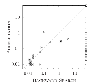
(a)

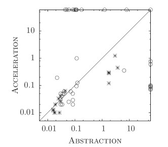
(b)

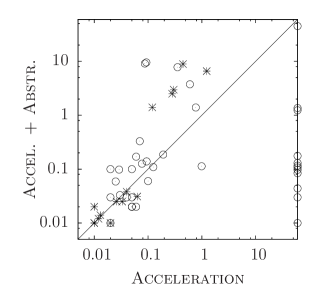
(c)

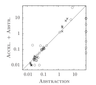
(d)

Figure 2: Comparison of time for different options of Backward Search. Stars and circles represent buggy and correct programs respectively.

In summary, the comparative analysis of timings presented in Figure2 confirms that acceleration indeed helps to avoid divergence for problematic programs where abstraction fails. The first comparison (Figure2(a)) highlights the benefits of using acceleration: Backward Search diverges on all 39 safe instances. Acceleration stops divergence in 23 cases, and moreover the overhead introduced by the preprocessing step does not affect unsafe instances. Figure2(b) shows that acceleration and abstraction are two complementary techniques, since mcmt times out in both cases but for two different sets of programs. Figure2(c) and Figure2(d) attest that acceleration and abstraction/refinement techniques mutually benefit from each other: with both techniques mcmt solves all the 55 benchmarks.

8 Conclusion and Future Work

We identified a class of transition relations involving array updates that can be accelerated, showed how it is possible to compute the accelerated transition and describe a solution for dealing with universal quantifiers arising from the acceleration process. Our paper lays theoretical foundations for this interesting research topic and confirms by our prototype experiments on challenging benchmarks its advantages over stand-alone verification approaches since it’s able to solve problems on which other techniques fail to converge.

As future directions, a challenging task is to enlarge the definability result of Theorem 6.1 so as to cover classes of transitions modeling more and more loop branches arising from concrete programs. In addition, one may want to consider more sophisticated strategies for instantiation in order to support acceleration. Considering increasing larger $\mathcal{S}$ or handling $\Sigma^{0}_{2}$-sentences when they belong to decidable fragments [15, 22] may lead to further improvements.

Appendix A Proof of Theorem 6.1

In this technical Appendix, we supply the proof of Theorem 6.1.

Proof.

As a preliminary observation, we notice that the bi-implications of the kind

$$(\bigvee_{n\geq 0}\psi(\underline{x},\bar{n}))\leftrightarrow\exists y\;(y\geq 0\wedge\psi(\underline{x},y))\leavevmode\nobreak\ .$$ (13)

are valid because we interpret our formulæ in the standard structure of natural numbers (enriched with extra free symbols).

As a second preliminary observation, we notice that (8) can be equivalently re-writtem in the form of a bi-implication as:

$$z=\kappa({\bf u}^{*}(\underline{x},y))\quad\leftrightarrow\quad[\;y=\iota(\underline{x},z)\leavevmode\nobreak\ \wedge\leavevmode\nobreak\ z=\kappa({\bf u}^{*}(\underline{x},\iota(\underline{x},z)))\;]\leavevmode\nobreak\ \leavevmode\nobreak\$$ (14)

(to see why (14) is equivalent to (8) it is sufficient to apply the logical laws of pure identity).

Let us fix a local ground assignment of the form (10); let ${\bf a}[{\bf d}]$ indicate the $s*|{\bf d}|$-tuple of terms $\{a_{i}(d_{j})\}_{1\leq i\leq s,1\leq j\leq|{\bf d}|}$; since $\phi_{L}$ and ${\bf t}$ are purely arithmetical over $\{\tilde{}{\bf c},{\bf d},{\bf a}(\kappa(\tilde{}{\bf c})),{\bf a}[{\bf d}]\}$, we have that they can be written as $\tilde{\phi}_{L}(\tilde{}{\bf c},{\bf d},{\bf a}(\kappa(\tilde{}{\bf c})),{\bf a}[{\bf d}])$, $\tilde{}{\bf t}(\tilde{}{\bf c},{\bf d},{\bf a}(\kappa(\tilde{}{\bf c})),{\bf a}[{\bf d}])$, respectively, where $\tilde{\phi}_{L},\tilde{}{\bf t}$ do not contain occurrences of the free function and constant symbols ${\bf a},{\bf c}$.

Claim. As a first step, we show by induction on $n$ that $\tau^{n}$ can be expressed as follows (we omit here and below the conjuncts $pc=l\wedge pc^{\prime}=l\wedge{\bf d}^{\prime}={\bf d}$ that do not play any role)

$$\bigwedge_{0\leq k<n}\tilde{\phi}_{L}({\bf u}^{*}(\tilde{}{\bf c},\bar{k}),{\bf d},{\bf a}(\kappa({\bf u}^{*}(\tilde{}{\bf c},\bar{k}))),{\bf a}[{\bf d}])\leavevmode\nobreak\ \wedge\leavevmode\nobreak\ \tilde{}{\bf c}^{\prime}={\bf u}^{*}(\tilde{}{\bf c},\bar{n})\leavevmode\nobreak\ \wedge\leavevmode\nobreak\ {\bf a}^{\prime}=\lambda j.\;F({\bf c},{\bf a},\bar{n},j)$$ (15)

where the tuple $F=F_{1},\dots,F_{s}$ of definable functions is given by

$$\begin{split}F_{h}({\bf c},{\bf a},y,j)\leavevmode\nobreak\ =\leavevmode\nobreak\ \lambda j.\leavevmode\nobreak\ \leavevmode\nobreak\ \mathtt{if}\leavevmode\nobreak\ \leavevmode\nobreak\ 0\leq\iota_{h}(\tilde{}{\bf c},j)<y\leavevmode\nobreak\ \wedge j=\kappa_{h}({\bf u}^{*}({\bf c},\iota_{h}(\tilde{}{\bf c},j)))\leavevmode\nobreak\ \mathtt{then}\;\\ \tilde{t}_{h}({\bf u}^{*}(\tilde{}{\bf c},\iota_{h}(\tilde{}{\bf c},j)),{\bf d},{\bf a}(\kappa({\bf u}^{*}(\tilde{}{\bf c},\iota_{h}(\tilde{}{\bf c},j)))),{\bf a}[{\bf d}])\;\mathtt{else}\;a_{h}[j]\end{split}$$ (16)

for $h=1,\dots,s$ (here $\iota_{1},\dots,\iota_{s}$ are the terms corresponding to $\kappa_{1},\dots,\kappa_{s}$ according to the definition of a selector for the iterator ${\bf u}$).

Proof of the Claim. For $n=1$, notice that $\tilde{\phi}_{L}({\bf u}^{*}(\tilde{}{\bf c},0),{\bf d},{\bf a}(\kappa({\bf u}^{*}(\tilde{}{\bf c},0))),{\bf a}[{\bf d}])$ is equivalent to $\tilde{\phi}_{L}(\tilde{}{\bf c},{\bf d},{\bf a}(\kappa(\tilde{}{\bf c})),{\bf a}[{\bf d}])$, that $\tilde{}{\bf c}^{\prime}={\bf u}^{*}(\tilde{}{\bf c},\bar{1})$ is equivalent to $\tilde{}{\bf c}^{\prime}={\bf u}(\tilde{}{\bf c})$ and that $\lambda j.\;F(\tilde{}{\bf c},{\bf d},{\bf a},\bar{1},j)=wr({\bf a},\kappa(\tilde{}{\bf c}),{\bf t}(\tilde{}{\bf c},{\bf d},{\bf a}(\kappa(\tilde{}{\bf c})),{\bf a}[{\bf d}]))$ holds (the latter because for every $h$, $\iota_{h}(\tilde{}{\bf c},j)=0\wedge j=\kappa_{h}({\bf u}^{*}({\bf c},\iota_{h}(\tilde{}{\bf c},j))$ is equivalent to $j=\kappa_{h}({\bf u}^{*}(\tilde{}{\bf c},0))=\kappa_{h}(\tilde{}{\bf c})$ by (14)).

For the induction step, we suppose the Claim holds for $n$ and show it for $n+1$. As a preliminary remark, notice that from (10), we get not only ${\bf d}^{\prime}={\bf d}$, but also ${\bf a}^{\prime}[{\bf d}^{\prime}]={\bf a}[{\bf d}]$, because of (v) of Definition 6.1. As a consequence, after $n$ iterations of $\tau$, the values ${\bf d},{\bf a}[{\bf d}]$ are left unchanged; thus, for notation simplicity, we will not display anymore below the dependence of $\phi_{L},\tilde{}{\bf t}$ on ${\bf d},{\bf a}[{\bf d}]$. We need to show that $\tau\circ\tau^{n}$ matches the required shape (15)-(16) with $n+1$ instead of $n$. After unraveling the definitions, this splits into three sub-claims, concerning the update of the ${\bf c}$, the guard and the update of the ${\bf a}$, respectively:

(i)

the equality ${\bf u}({\bf u}^{*}(\tilde{}{\bf c},\bar{n}))={\bf u}^{*}(\tilde{}{\bf c},\overline{n+1})$ is valid;

(ii)

$$\bigwedge_{0\leq k<n}\tilde{\phi}_{L}({\bf u}^{*}(\tilde{}{\bf c},\bar{k}),{\bf a}(\kappa({\bf u}^{*}(\tilde{}{\bf c},\bar{k}))))\leavevmode\nobreak\ \wedge\leavevmode\nobreak\ \tilde{\phi}_{L}({\bf u}^{*}(\tilde{}{\bf c},\overline{n}),\lambda j.\;F({\bf c},{\bf a},\bar{n},j)(\kappa({\bf u}^{*}(\tilde{}{\bf c},\overline{n}))))$$

is equivalent to

$$\bigwedge_{0\leq k<n+1}\tilde{\phi}_{L}({\bf u}^{*}({\bf c},\bar{k}),{\bf a}(\kappa({\bf u}^{*}({\bf c},\bar{k}))));$$

(iii)

$wr(\lambda j.\,F({\bf c},{\bf a},\bar{n},j),\kappa({\bf u}^{*}(\tilde{}{\bf c},\overline{n})),\tilde{}{\bf t}({\bf u}^{*}(\tilde{}{\bf c},\overline{n}),\lambda j.\,F({\bf c},{\bf a},\bar{n},j)(\kappa({\bf u}^{*}(\tilde{}{\bf c},\bar{n}))))$ is the same function as $\lambda j.\;F({\bf c},{\bf a},\overline{n+1},j)$.

Indeed statement (i) is trivial, because ${\bf u}({\bf u}^{*}(\tilde{}{\bf c},\bar{n}))={\bf u}({\bf u}^{n}(\tilde{}{\bf c}))={\bf u}^{n+1}(\tilde{}{\bf c})={\bf u}^{*}(\tilde{}{\bf c},\overline{n+1})$ holds by (7).

To show (ii), it is sufficient to check that

$${\bf a}(\kappa({\bf u}^{*}(\tilde{}{\bf c},\overline{n})))\leavevmode\nobreak\ =\leavevmode\nobreak\ \lambda j.\;F({\bf c},{\bf a},\bar{n},j)(\kappa({\bf u}^{*}(\tilde{}{\bf c},\overline{n})))$$ (17)

is true. In turn, this follows from (16) and the validity of the following implications (varying $h=1,\dots,s$)

$$\iota_{h}(\tilde{}{\bf c},j)\neq\bar{n}\leavevmode\nobreak\ \to\leavevmode\nobreak\ j\neq\kappa_{h}({\bf u}^{*}(\tilde{}{\bf c},\overline{n}))\leavevmode\nobreak\$$ (18)

(in fact, $a_{h}$ and $F_{h}$ can possibly differ only for the $j$ satisfying $0\leq\iota_{h}(\tilde{}{\bf c},j)<\bar{n}$, i.e. in particular for the $j$ such that $\iota_{h}(\tilde{}{\bf c},j)\neq n$). To see why (18) is valid, notice that in view of (8), what (18) says is that we cannot have simultaneously both $\iota_{h}(\tilde{}{\bf c},j)=\overline{n}$ and $\iota_{h}(\tilde{}{\bf c},j)=\bar{m}$, for some $m\neq n$: indeed it is so by the definition of a function.

It remains to prove (iii); in view of (17) just shown, we need to check that

$$wr(\lambda j.\,F({\bf c},{\bf a},\bar{n},j),\kappa({\bf u}^{*}(\tilde{}{\bf c},\overline{n})),\tilde{}{\bf t}({\bf u}^{*}(\tilde{}{\bf c},\overline{n}),{\bf a}(\kappa({\bf u}^{*}(\tilde{}{\bf c},\overline{n})))))$$

is the same as $\lambda j.\;F({\bf c},{\bf a},\overline{n+1},j)$. For every $h=1,\dots,s$, this is split into three cases, corresponding to the validity check for the three implications:

$$\leavevmode\nobreak\ \leavevmode\nobreak\ \leavevmode\nobreak\ \leavevmode\nobreak\ i_{h}(\tilde{}{\bf c},j)<\bar{n}\to wr(\lambda j.\,F_{h}({\bf c},{\bf a},\bar{n},j),\kappa_{h}({\bf u}^{*}(\tilde{}{\bf c},\overline{n})),\tilde{t}_{h})(j)=F_{h}({\bf c},{\bf a},\overline{n+1},j)$$

$$\leavevmode\nobreak\ \leavevmode\nobreak\ \leavevmode\nobreak\ \leavevmode\nobreak\ i_{h}(\tilde{}{\bf c},j)=\overline{n}\to wr(\lambda j.\,F_{h}({\bf c},{\bf a},\bar{n},j),\kappa_{h}({\bf u}^{*}(\tilde{}{\bf c},\overline{n})),\tilde{t}_{h})(j)=F_{h}({\bf c},{\bf a},\overline{n+1},j)$$

$$\leavevmode\nobreak\ \leavevmode\nobreak\ \leavevmode\nobreak\ \leavevmode\nobreak\ i_{h}(\tilde{}{\bf c},j)>\overline{n}\to wr(\lambda j.\,F_{h}({\bf c},{\bf a},\bar{n},j),\kappa_{h}({\bf u}^{*}(\tilde{}{\bf c},\overline{n})),\tilde{t}_{h})(j)=F_{h}({\bf c},{\bf a},\overline{n+1},j)$$

where we wrote simply $\tilde{t}_{h}$ instead of $\tilde{t}_{h}({\bf u}^{*}(\tilde{}{\bf c},\overline{n}),{\bf a}(\kappa({\bf u}^{*}(\tilde{}{\bf c},\overline{n}))))$. However, keeping in mind (18) and (14), the three implications can be rewritten as follows (the second one is split into two subcases)

$$i_{h}(\tilde{}{\bf c},j)<\bar{n}\to\,F_{h}({\bf c},{\bf a},\bar{n},j)=F_{h}({\bf c},{\bf a},\overline{n+1},j)$$

$$i_{h}(\tilde{}{\bf c},j)=\overline{n}\wedge j=\kappa_{h}({\bf u}^{*}({\bf c},\iota_{h}(\tilde{}{\bf c},j)))\to\tilde{t}_{h}=F_{h}({\bf c},{\bf a},\overline{n+1},j)$$

$$i_{h}(\tilde{}{\bf c},j)=\overline{n}\wedge j\neq\kappa_{h}({\bf u}^{*}({\bf c},\iota_{h}(\tilde{}{\bf c},j)))\to\,F_{h}({\bf c},{\bf a},\bar{n},j)=F_{h}({\bf c},{\bf a},\overline{n+1},j)$$

$$i_{h}(\tilde{}{\bf c},j)>\overline{n}\to\,F_{h}({\bf c},{\bf a},\bar{n},j)=F_{h}({\bf c},{\bf a},\overline{n+1},j)$$

The above four implications all hold by the definitions (16) of the $F_{h}$.

Proof of Theorem 6.1 (continued). As a consequence of the Claim, since the formula

$$\bigwedge_{0\leq k<n}\tilde{\phi}_{L}({\bf u}^{*}(\tilde{}{\bf c},\bar{k}),{\bf d},{\bf a}(\kappa({\bf u}^{*}(\tilde{}{\bf c},\bar{k}))),{\bf a}[{\bf d}])$$

is equivalent to $\forall z\leavevmode\nobreak\ (0\leq z<\bar{n}\to\tilde{\phi}_{L}({\bf u}^{*}(\tilde{}{\bf c},z),{\bf d},{\bf a}(\kappa({\bf u}^{*}({\bf c},z))),{\bf a}[{\bf d}]),$ we can use (13) to express $\tau^{+}$ as

$$\exists y>0\left(\begin{split}\forall z\leavevmode\nobreak\ (0\leq\!z\!<y\!\to\!\tilde{\phi}_{L}({\bf u}^{*}(\tilde{}{\bf c},z),{\bf d},{\bf a}(\kappa({\bf u}^{*}({\bf c},z))),{\bf a}[{\bf d}])\wedge{\bf d}^{\prime}={\bf d}\,\wedge\\ \wedge\leavevmode\nobreak\ pc=l\leavevmode\nobreak\ \wedge\leavevmode\nobreak\ pc^{\prime}=l\leavevmode\nobreak\ \wedge\leavevmode\nobreak\ \tilde{}{\bf c}^{\prime}={\bf u}^{*}(\tilde{}{\bf c},y)\leavevmode\nobreak\ \wedge\leavevmode\nobreak\ {\bf a}^{\prime}=\lambda j.\;F({\bf c},{\bf a},y,j)\end{split}\right)$$ (19)

The latter shows that $\tau^{+}$ is a $\Sigma^{0}_{2}$-assignment, as desired. $\hfill\dashv$

∎

Appendix B A worked out example

Simple assignements might not be sufficient for nested loops where an array is scanned by a couple of counters, one of which is kept fixed (think for instance of inner loops of sorting algorithms). To cope with these more complicated cases, we introduce a larger class of assignments (these assignments are still local, hence covered by Theorem 6.1). We call simple+ the ground assignments of the form

$$pc=l\;\wedge\;\phi_{L}({\tt c},{\bf d},{\bf a})\;\wedge\;pc^{\prime}=l\wedge{\tt c}^{\prime}={\tt c}\pm 1\,\wedge\,{\bf d}^{\prime}={\bf d}\;\wedge\;{\bf a}^{\prime}=wr({\bf a},{\tt c},{\bf t}({\tt c},{\bf d},{\bf a}))$$ (20)

where (i) ${\bf d}=d_{1},\dots,d_{l}$ is a tuple of integer constants, (ii) the first occurrence of ${\tt c}$ in $wr({\bf a},{\tt c},{\bf t}({\tt c},{\bf d},{\bf a}))$ stands for a tuple of terms all identical to ${\tt c}$, (iii) the guard $\phi_{L}$ contains the conjuncts ${\tt c}\neq d_{i}$ ($1\leq i\leq l$), and (iv) $\phi_{L},{\bf t}$ are purely arithmetical over ${\tt c},{\bf d},a_{1}[{\tt c}],\dots a_{s}[{\tt c}],a_{1}[d_{1}],\dots,a_{s}[d_{l}]$. Basically, simple+ local ground assignments differ from plain simple ones just because there are some ‘idle’ indices ${\bf d}$; in addition, the counter ${\tt c}$ can also be decremented.

The accelerated transition for (20) computed by Theorem 6.1 can be re-written as follows (we write $j\in[{\tt c},{\tt c}\pm k]$ for ${\tt c}\leq j\leq{\tt c}+k$ or ${\tt c}-k\leq j\leq{\tt c}$, depending on whether we have increment or decrement in (20)):

$$\exists k\left(\begin{split}k>0\leavevmode\nobreak\ \wedge\leavevmode\nobreak\ pc=l\leavevmode\nobreak\ \wedge\leavevmode\nobreak\ \forall j\leavevmode\nobreak\ (j\in[{\tt c},{\tt c}\pm k]\to\phi_{L}(j,{\bf d},{\bf a}))\leavevmode\nobreak\ \wedge\leavevmode\nobreak\ pc^{\prime}=l\leavevmode\nobreak\ \wedge\leavevmode\nobreak\ {\bf d}^{\prime}={\bf d}\leavevmode\nobreak\ \wedge\\ \wedge\leavevmode\nobreak\ {\tt c}^{\prime}={\tt c}\pm k\leavevmode\nobreak\ \wedge\leavevmode\nobreak\ {\bf a}^{\prime}=\lambda j.\;(\mathtt{if}\leavevmode\nobreak\ j\in[{\tt c},{\tt c}\pm k]\leavevmode\nobreak\ \mathtt{then}\leavevmode\nobreak\ {\bf t}(j,{\bf d},{\bf a})\leavevmode\nobreak\ \mathtt{else}\leavevmode\nobreak\ {\bf a}[j])\end{split}\right)$$ (21)

To show how acceleration and abstraction/refinement techniques can mutually benefit from each other, consider the procedure allDiff, represented by the all diff 2 entry in TableLABEL:tab:experiments. This function tests whether all entries of the array ${\tt a}$ are pairwise different:

$${\sf function}\leavevmode\nobreak\ {\tt allDiff}\leavevmode\nobreak\ (\leavevmode\nobreak\ {\sf int}\leavevmode\nobreak\ {\tt a}[{\tt N}]\leavevmode\nobreak\ ):\leavevmode\nobreak\$$

$$1\leavevmode\nobreak\ \leavevmode\nobreak\ {\tt r}={\sf true};$$

$$2\leavevmode\nobreak\ \leavevmode\nobreak\ {\sf for}\leavevmode\nobreak\ ({\tt i}=1;\leavevmode\nobreak\ {\tt i}<{\tt N}\wedge{\tt r};{\tt i}\text{+}\text{+})\leavevmode\nobreak\$$

$$3\leavevmode\nobreak\ \leavevmode\nobreak\ \leavevmode\nobreak\ \leavevmode\nobreak\ \leavevmode\nobreak\ {\sf for}\leavevmode\nobreak\ ({\tt j}={\tt i}\text{-}1;{\tt j}\geq 0\wedge{\tt r};{\tt j}\text{-}\text{-})\leavevmode\nobreak\$$

$$4\leavevmode\nobreak\ \leavevmode\nobreak\ \leavevmode\nobreak\ \leavevmode\nobreak\ \leavevmode\nobreak\ \leavevmode\nobreak\ \leavevmode\nobreak\ {\sf if}\leavevmode\nobreak\ ({\tt a}[{\tt i}]={\tt a}[{\tt j}])\leavevmode\nobreak\ {\tt r}={\sf false};$$

$$5\leavevmode\nobreak\ \leavevmode\nobreak\ {\sf assert}\leavevmode\nobreak\ \left({\tt r}\rightarrow\left(\forall x,y(0\leq x<y<{\tt N})\rightarrow({\tt a}[x]\neq{\tt a}[y])\right)\right)$$

This function is represented by the transition system specified below (in the specification, we omit identical updates to improve readability).

$$I({\bf v})=\left(r=0\wedge{\tt i}=1\wedge{\tt j}=0\wedge pc=l_{1}\right)$$

$$U({\bf v})=pc=l_{4}\wedge\exists x,y.\left(0\leq x<y<{\tt a.Length}\wedge a[x]=a[y]\right)$$

$$\tau_{1}=\left(\begin{aligned} &pc=l_{1}\wedge{\tt i}\leq{\tt a.Length}\wedge r=0\leavevmode\nobreak\ \wedge\\ &pc^{\prime}=l_{2}\wedge{\tt j}^{\prime}={\tt i}-1\end{aligned}\right)$$

$$\tau_{2}=\left(\begin{aligned} &pc=l_{1}\wedge{\tt i}>{\tt a.Length}\leavevmode\nobreak\ \wedge\\ &pc^{\prime}=l_{4}\end{aligned}\right)$$

$$\tau_{3}=\left(\begin{aligned} &pc=l_{1}\wedge r=1\leavevmode\nobreak\ \wedge\\ &pc^{\prime}=l_{4}\end{aligned}\right)$$

$$\tau_{4}=\left(\begin{aligned} &pc=l_{3}\leavevmode\nobreak\ \wedge\\ &pc^{\prime}=l_{1}\wedge{\tt i}^{\prime}={\tt i}+1\end{aligned}\right)$$

$$\tau_{5}=\left(\begin{aligned} &pc=l_{2}\wedge r=0\wedge{\tt j}\geq 0\wedge a[{\tt i}]=a[{\tt j}]\leavevmode\nobreak\ \wedge\\ &pc^{\prime}=l_{2}\wedge{\tt j}^{\prime}={\tt j}-1\wedge r=1\end{aligned}\right)$$

$$\tau_{6}=\left(\begin{aligned} &pc=l_{2}\wedge r=0\wedge{\tt j}\geq 0\wedge a[{\tt i}]\neq a[{\tt j}]\leavevmode\nobreak\ \wedge\\ &pc^{\prime}=l_{2}\wedge{\tt j}^{\prime}={\tt j}-1\end{aligned}\right)$$

$$\tau_{7}=\left(\begin{aligned} &pc=l_{2}\wedge j<0\leavevmode\nobreak\ \wedge\\ &pc^{\prime}=l_{3}\end{aligned}\right)$$

$$\tau_{8}=\left(\begin{aligned} &pc=l_{2}\wedge r=1\leavevmode\nobreak\ \wedge\\ &pc^{\prime}=l_{3}\end{aligned}\right)$$

For this problem, the transition we want to accelerate is $\tau_{6}$. Accelerating transition $\tau_{6}$ is not sufficient to avoid divergence caused by the outer loop, though. On the other side, accelerating the inner loop simplifies the problem, which can be successfully verified by the model checker by exploiting abstraction/refinement techniques in 1.36 seconds (see TableLABEL:tab:experiments for more details).

The acceleration of transition $\tau_{6}$ requires simple+-assignements (implemented in the current release of mcmt). We follow mcmt implementation quite closely to explain what happens.

As a first observation, mcmt specification language requires that whenever two counters ${\tt i}$ and ${\tt j}$ both occur in array applications $a[{\tt i}],a[{\tt j}]$ (like in $\tau_{6}$ above), the guard of the transition must contain either the literal ${\tt i}={\tt j}$ or the literal ${\tt i}\neq{\tt j}$. Thus such transitions must be duplicated; in our case, the copy of $\tau_{6}$ with ${\tt i}={\tt j}$ can be ignored because it has an inconsistent guard. The copy with ${\tt i}{\mathtt{\neq}}{\tt j}$ in the guard satisfies the conditions for being a simple+-assignment. Thus, its acceleration, according to (21), can be written as

$$\exists k\left(\begin{split}k>0\leavevmode\nobreak\ \wedge\leavevmode\nobreak\ \forall j\leavevmode\nobreak\ (j\in[{\tt j},{\tt j}\pm k]\to{\tt i}\neq j\wedge r=0\wedge j\geq 0\wedge a[{\tt i}]\neq a[j])\leavevmode\nobreak\ \wedge\leavevmode\nobreak\ \\ \wedge\leavevmode\nobreak\ pc=2\leavevmode\nobreak\ \wedge pc^{\prime}=2\leavevmode\nobreak\ \wedge\leavevmode\nobreak\ {\tt i}^{\prime}={\tt i}\leavevmode\nobreak\ \wedge\leavevmode\nobreak\ r^{\prime}=r\leavevmode\nobreak\ \wedge\leavevmode\nobreak\ {\tt j}^{\prime}={\tt j}\pm k\leavevmode\nobreak\ \wedge\leavevmode\nobreak\ {\bf a}^{\prime}={\bf a}\end{split}\right)$$

In the current release, mcmt is able to compute by itself the above accelerated transition and thus to certify safety of allDiff procedure.

Appendix C Experimental evaluation

Complete statistics for the experiments performed with mcmt are reported in TableLABEL:tab:experiments. Benchmarks have been taken from different sources:

• The benchmarks “filter test”, “max in array test”, “filter”, “max in array 1”, “max in array 2”, “max in array 3” have been taken and/or adapted from programs on http://proval.lri.fr/.

• The “heap as array” program has been suggested by K. Rustan M. Leino and it is reported in FigureLABEL:fig:heap_program.

• all the programs $pN$ have been taken from “I. Dillig, T. Dillig, and A. Aiken. Fluid updates: Beyond strong vs. weak updates. In ESOP, pages 246-266, 2010.”.

• The “bubble sort” example comes from the “Eureka” project http://www.ai-lab.it/eureka and has been used as a benchmark in the paper “A. Armando, M. Benerecetti, and J. Mantovani. Abstraction refinement of linear programs with arrays. In TACAS, pages 373-388, 2007.”

• “all diff 1” and “all diff 2” have been suggested by Madhusudan Parthasarath and his group. They represent two different encoding of an algorithm that initializes an array to different values and then check if the array has been correctly initialized.

• “compare”, “copy”, “find 1”, “find 2”, “init”, “init test”, “partition” have been taken/adapted from “Krystof Hoder, Laura Kovács, Andrei Voronkov: Interpolation and Symbol Elimination in Vampire. In IJCAR, pages 188-195, 2010”.

• The “linear search” program is used as a running example on the book “Aaron R. Bradley, Zohar Manna: The calculus of computation - decision procedures with applications to verification. Springer 2007, pp. I-XV, 1-366”.

• “selection sort” example has been used in “M. N. Seghir, A. Podelski, and T. Wies. Abstraction Refinement for Quantified Array Assertions. In SAS, pages 3-18, 2009.”

• “strcmp”, “strcpy” and “strlen” have been adapted from the standard string C library.

The benchmarks named with “ * test ” refer to benchmarks with quantified assertions substituted by a for loop. For those programs, the postcondition does not have quantifiers: in these benchmarks it is even harder to come up with a quantified safe inductive invariant to prove that the program is correct. Thus, it is a remarkable fact that our tool can automatically synthetize such invariants.

Program						Status	No options	Abstraction	Acceleration	Accel. + Abstr.
filter test						safe	$\times$	0.08	$\times$	0.08
heap as array	safe	$\times$	0.12	$\times$	0.12
init test	safe	$\times$	11.72	$\times$	0.16
max in array test	safe	$\times$	0.18	$\times$	0.18
p01	safe	$\times$	$\times$	0.09	9.08
p02	safe	$\times$	$\times$	0.09	9.52
p03	safe	$\times$	0.11	0.09	0.14
p08	safe	$\times$	0.12	0.12	0.11
p09	safe	$\times$	0.12	0.99	0.11
p14	safe	$\times$	6.39	0.35	7.78
p17	safe	$\times$	0.02	0.19	0.19
p04	unsafe	0.02	0.03	0.03	0.02
p10	unsafe	0.07	0.04	0.06	0.03
p11	unsafe	0.02	0.03	0.04	0.04
p15	unsafe	1.4	1.74	0.3	2.97
p16	unsafe	4.27	3.70	0.45	8.89
p18	unsafe	0.01	0.02	0.01	0.01
p19	unsafe	0.02	0.02	0.01	0.01
p20	unsafe	0.02	0.02	0.03	0.02
p22	unsafe	0.02	0.03	0.02	0.17
all diff 1						safe	$\times$	$\times$	0.08	0.13
all diff 2	safe	$\times$	$\times$	$\times$	1.36
bubble sort	safe	$\times$	1.23	$\times$	1.23
compare	safe	$\times$	0.04	$\times$	0.04
copy	safe	$\times$	0.03	0.03	0.03
filter	safe	$\times$	0.11	$\times$	0.11
find 1	safe	$\times$	0.06	$\times$	0.06
find 2	safe	$\times$	0.07	0.06	0.17
init	safe	$\times$	0.08	0.03	0.1
linear search	safe	$\times$	0.04	0.05	0.02
max in array 1	safe	$\times$	0.1	$\times$	0.1
max in array 2	safe	$\times$	0.11	$\times$	0.13
max in array 3	safe	$\times$	0.06	$\times$	0.01
minusN	safe	$\times$	$\times$	0.77	1.4
partition	safe	$\times$	0.05	$\times$	0.03
selection sort	safe	$\times$	7.87	$\times$	45.07
strcat 1	safe	$\times$	$\times$	$\times$	3.5
strcat 2	safe	$\times$	$\times$	$\times$	3.62
strcmp	safe	$\times$	0.04	0.06	0.02
strcpy	safe	$\times$	0.03	0.02	0.01
strlen	safe	$\times$	$\times$	0.1	0.06
p01	safe	$\times$	0.08	0.02	0.1
p02	safe	$\times$	0.08	0.05	0.1
p03	safe	$\times$	0.03	0.02	0.03
p08	safe	$\times$	0.03	0.05	0.03
p09	safe	$\times$	0.03	0.04	0.03
p18	safe	$\times$	$\times$	0.07	0.33
p20	safe	$\times$	0.04	0.05	0.02
p04	unsafe	0.07	0.02	0.01	0.01
p11	unsafe	0.01	0.02	0.02	0.01
p14	unsafe	0.31	1.79	0.28	2.5
p15	unsafe	0.09	1.77	0.12	1.4
p16	unsafe	0.11	2.97	1.23	6.57
p17	unsafe	0.02	0.03	0.01	0.02
p19	unsafe	0.02	0.02	0.01	0.01

References

- [1] P.A. Abdulla, G. Delzanno, N.B. Henda, and A. Rezine. Regular model checking without transducers. In TACAS, volume 4424 of LNCS, pages 721–736, 2007.
- [2] P.A. Abdulla, G. Delzanno, and A. Rezine. Parameterized verification of infinite-state processes with global conditions. In CAV, LNCS, pages 145–157, 2007.
- [3] F. Alberti, R. Bruttomesso, S. Ghilardi, S. Ranise, and N. Sharygina. Lazy Abstraction with Interpolants for Arrays. In LPAR, pages 46–61, 2012.
- [4] F. Alberti, R. Bruttomesso, S. Ghilardi, S. Ranise, and N. Sharygina. SAFARI: SMT-Based Abstraction for Arrays with Interpolants. In CAV, 2012.
- [5] F. Alberti, S. Ghilardi, E. Pagani, S. Ranise, and G.P. Rossi. Universal Guards, Relativization of Quantifiers, and Failure Models in Model Checking Modulo Theories. JSAT, pages 29–61, 2012.
- [6] Thomas Ball and Sriram K. Rajamani. The slam toolkit. In CAV, pages 260–264, 2001.
- [7] Clark Barrett, Aaron Stump, and Cesare Tinelli. The SMT-LIB Standard: Version 2.0. www.SMT-LIB.org, 2010.
- [8] G. Behrmann, J. Bengtsson, A. David, K.G. Larsen, P. Pettersson, and W. Yi. Uppaal implementation secrets. In FTRTFT, pages 3–22, 2002.
- [9] Dirk Beyer, Thomas A. Henzinger, Rupak Majumdar, and Andrey Rybalchenko. Path invariants. In PLDI, pages 300–309, 2007.
- [10] Cristina Borralleras, Salvador Lucas, Albert Oliveras, Enric Rodríguez-Carbonell, and Albert Rubio. Sat modulo linear arithmetic for solving polynomial constraints. J. Autom. Reasoning, 48(1):107–131, 2012.
- [11] M. Bozga, C. Girlea, and R. Iosif. Iterating octagons. In TACAS, LNCS, pages 337–351, 2009.
- [12] M. Bozga, P. Habermehl, R. Iosif, F. Konecný, and T. Vojnar. Automatic verification of integer array programs. In CAV, pages 157–172, 2009.
- [13] M. Bozga, R. Iosif, and F. Konecny. Fast acceleration of ultimately periodic relations. In CAV, LNCS, 2010.
- [14] M. Bozga, R. Iosif, and Y. Lakhnech. Flat parametric counter automata. Fundamenta Informaticae, (91):275–303, 2009.
- [15] A.R. Bradley, Z. Manna, and H.B. Sipma. What’s decidable about arrays? In VMCAI, pages 427–442, 2006.
- [16] Nicolas Caniart, Emmanuel Fleury, Jérôme Leroux, and Marc Zeitoun. Accelerating interpolation-based model-checking. In TACAS, pages 428–442, 2008.
- [17] Alessandro Cimatti, Alberto Griggio, and Roberto Sebastiani. Efficient generation of craig interpolants in satisfiability modulo theories. ACM Trans. Comput. Log., 12(1):7, 2010.
- [18] E.M. Clarke, O. Grumberg, S. Jha, Y. Lu, and H. Veith. Counterexample-Guided Abstraction Refinement. In CAV, pages 154–169, 2000.
- [19] H. Comon and Y. Jurski. Multiple counters automata, safety analysis and presburger arithmetic. In CAV, volume 1427 of LNCS, pages 268–279. Springer, 1998.
- [20] A. Finkel and J. Leroux. How to compose presburger-accelerations: Applications to broadcast protocols. In FST TCS ‘02, pages 145–156. Springer, 2002.
- [21] C. Flanagan and S. Qadeer. Predicate abstraction for software verification. In POPL, pages 191–202, 2002.
- [22] Y. Ge and L. de Moura. Complete instantiation for quantified formulas in satisfiabiliby modulo theories. In CAV, pages 306–320, 2009.
- [23] S. Ghilardi and S. Ranise. MCMT: A Model Checker Modulo Theories. In IJCAR, pages 22–29, 2010.
- [24] S. Graf and H. Saïdi. Construction of Abstract State Graphs with PVS. In CAV, pages 72–83, 1997.
- [25] M. Hendriks and K.G. Larsen. Exact acceleration of real-time model checking. Electr. Notes Theor. Comput. Sci., 65(6):120–139, 2002.
- [26] H. Hojjat, R. Josif, F. Konecny, V. Kuncak, and P. Rümmer. On accelerating interpolants. In ATVA, 2012.
- [27] R. Jhala and K.L. McMillan. Array Abstractions from Proofs. In CAV, 2007.
- [28] L. Kovács and A. Voronkov. Interpolation and Symbol Elimination. In CADE, 2009.
- [29] Daniel Larraz, Enric Rodríguez-Carbonell, and Albert Rubio. Smt-based array invariant generation. In VMCAI, pages 169–188, 2013.
- [30] K.L. McMillan. Lazy Abstraction with Interpolants. In CAV, 2006.
- [31] K.L. McMillan. Quantified Invariant Generation Using an Interpolating Saturation Prover. In TACAS, 2008.
- [32] G. Nelson and D.C. Oppen. Simplification by cooperating decision procedures. ACM Transaction on Programming Languages and Systems, 1(2):245–257, 1979.
- [33] M. N. Seghir, A. Podelski, and T. Wies. Abstraction Refinement for Quantified Array Assertions. In SAS, pages 3–18, 2009.
- [34] S. Srivastava and S. Gulwani. Program Verification using Templates over Predicate Abstraction. In PLDI, 2009.
- [35] C. Tinelli and M. T. Harandi. A new correctness proof of the Nelson-Oppen combination procedure. In Proc. of FroCoS 1996, pages 103–119. Kluwer, 1996.