Optimizing snake locomotion in the plane. II. Large transverse friction

Abstract

We determine analytically the form of optimal snake locomotion when the coefficient of transverse friction is large, the typical regime for biological and robotic snakes. We find that the optimal snake motion is a retrograde traveling wave, with a wave amplitude that decays as the -1/4 power of the coefficient of transverse friction. This result agrees well with our numerical computations.


Keywords: snake; friction; sliding; locomotion; optimization.

I Introduction

In AlbenSnake2013I we considered the problem of optimizing snake locomotion in the plane numerically. The mechanics of snake locomotion has been described previously by biologists and engineers, and modeled by applied mathematicians (gray1950kinetics, ; GuMa2008a, ; HuNiScSh2009a, ; HaCh2010b, ; MaHu2012a, ; HuSh2012a, ). As with other terrestrial locomoting animals (dickinson2000animals, ), a terrestrial snake pushes against the ground with its body, and obtains a reaction force from the ground which propels it forward. However, a wide range of possible kinematics can be employed, and determining which are most effective (i.e. efficient) in different environments, and why, has been a major theme of locomotion studies (BeKoSt2003a, ; AvGaKe2004a, ; TaHo2007a, ; fu2007theory, ; spagnolie2010optimal, ; crowdy2011two, ; lighthill1975mathematica, ; childress1981mechanics, ; sparenberg1994hydrodynamic, ; alben2009passive, ; michelin2009resonance, ; peng2012bb, ).

A first approximation to snake locomotion is to consider motions confined to two dimensions GuMa2008a ; HuNiScSh2009a ; HuSh2012a . Here the reaction force in the plane of snake motion is due to friction, and Coulomb friction provides a simple model. Hu and Shelley HuNiScSh2009a ; HuSh2012a emphasized the importance of frictional anisotropy in snake locomotion. In particular, they found that when the curvature of the snake backbone is prescribed as a sinusoidal traveling wave, high speed and efficiency is obtained when the coefficient of transverse friction is large compared to the coefficient of forward friction. Jing and Alben JiAl2013 found that the same holds for two- and three-link snakes. In biological snakes, the ratio of transverse to forward friction is thought to be greater than one HuNiScSh2009a ; HuSh2012a , although how much greater is not clear. In HuNiScSh2009a ; HuSh2012a , a ratio of only 1.7 was measured for anaesthetized snakes. These works noted that active snakes use their scales to increase frictional anisotropy, so the ratio in locomoting snakes is potentially much larger, and indeed, a ratio of 10 was found to give better agreement between the Coulomb friction model and a biological snake HuSh2012a . Wheeled snake robots have been employed very successfully for locomotion hirosebiologically ; hopkins2009survey , and for most wheels the frictional coefficient ratio (with forward friction defined by the rolling resistance coefficient of the wheel) is much greater than 10 persson2000sliding .

In this paper, we develop an analytical solution for the optimal locomotion of a snake in the plane, when the ratio of transverse to forward friction is large. We make few assumptions on the snake kinematics at the outset, but use numerical computations from AlbenSnake2013I to provide guiding intuition. We find first that the optimal form of the prescribed backbone curvature is a traveling wave. We then find that the root-mean-square (RMS) amplitude of the curvature should decay as the $-1/4$ power of the ratio of transverse to forward friction coefficients. Surprisingly, any periodic traveling wave motion can achieve the optimal efficiency, subject to the aforementioned restriction on its RMS amplitude, and to the requirement that its wavelength, normalized by the snake length, tend to zero. In the limit of large transverse friction, the power required to move a snake optimally is simply that needed to tow a straight snake forward.

II Model

We use the same frictional snake model as (HuNiScSh2009a, ; HuSh2012a, ; JiAl2013, ; AlbenSnake2013I, ), so we only summarize it here. The snake’s position is given by $\mathbf{X}(s,t)=(x(s,t),y(s,t))$, a planar curve which is parametrized by arc length $s$ and varies with time $t$. A schematic diagram is shown in figure 1.

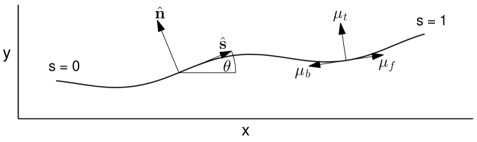
Figure 1: Schematic diagram of snake position, parametrized by arc length $s$ (nondimensionalized by snake length), at an instant in time. The tangent angle and unit vectors tangent and normal to the curve at a point are labeled. Vectors representing forward, backward and transverse velocities are shown with the corresponding friction coefficients $\mu_{f}$, $\mu_{b}$, and $\mu_{t}$.

The unit vectors tangent and normal to the curve are $\hat{\mathbf{s}}$ and $\hat{\mathbf{n}}$ respectively. The tangent angle and curvature are denoted $\theta(s,t)$ and $\kappa(s,t)$, and satisfy $\partial_{s}x=\cos\theta$, $\partial_{s}y=\sin\theta$, and $\kappa=\partial_{s}\theta$. We consider the problem of prescribing the curvature of the snake as a function of time, $\kappa(s,t)$, in order to obtain efficient locomotion. When $\kappa(s,t)$ is prescribed, the tangent angle and position are obtained by integration:

$$\theta(s,t) =\theta_{0}(t)+\int_{0}^{s}\kappa(s^{\prime},t)ds^{\prime},$$ (1)

$$x(s,t) =x_{0}(t)+\int_{0}^{s}\cos\theta(s^{\prime},t)ds^{\prime},$$ (2)

$$y(s,t) =y_{0}(t)+\int_{0}^{s}\sin\theta(s^{\prime},t)ds^{\prime}.$$ (3)

The trailing-edge position $(x_{0},y_{0})$ and tangent angle $\theta_{0}$ are determined by the force and torque balance for the snake, i.e. Newton’s second law:

$$\int_{0}^{L}\rho\partial_{tt}xds =\int_{0}^{L}f_{x}ds,$$ (4)

$$\int_{0}^{L}\rho\partial_{tt}yds =\int_{0}^{L}f_{y}ds,$$ (5)

$$\int_{0}^{L}\rho\mathbf{X}^{\perp}\cdot\partial_{tt}\mathbf{X}ds =\int_{0}^{L}\mathbf{X}^{\perp}\cdot\mathbf{f}ds.$$ (6)

Here $\rho$ is the snake’s mass per unit length and $L$ is the snake length. The snake is locally inextensible, and $\rho$ and $L$ are constant in time. $\mathbf{f}$ is the force per unit length on the snake due to Coulomb friction with the ground HuNiScSh2009a :

$$\mathbf{f}(s,t)=-\rho g\mu_{t}\left(\widehat{\partial_{t}{\mathbf{X}}}\cdot\hat{\mathbf{n}}\right)\hat{\mathbf{n}}-\rho g\left(\mu_{f}H(\widehat{\partial_{t}{\mathbf{X}}}\cdot\hat{\mathbf{s}})+\mu_{b}(1-H(\widehat{\partial_{t}{\mathbf{X}}}\cdot\hat{\mathbf{s}}))\right)\left(\widehat{\partial_{t}{\mathbf{X}}}\cdot\hat{\mathbf{s}}\right)\hat{\mathbf{s}}.$$ (7)

Here $H$ is the Heaviside function and the hats denote normalized vectors. When $\|\partial_{t}{\mathbf{X}}\|=\mathbf{0}$ we define $\widehat{\partial_{t}{\mathbf{X}}}$ to be $\mathbf{0}$. According to (7) the snake experiences friction with different coefficients for motions in different directions. The frictional coefficients are $\mu_{f}$, $\mu_{b}$, and $\mu_{t}$ for motions in the forward ($\hat{\mathbf{s}}$), backward ($-\hat{\mathbf{s}}$), and transverse (i.e. normal) directions ($\pm\hat{\mathbf{n}}$), respectively. In general the snake velocity at a given point has both tangential and normal components, and the frictional force density has components acting in each direction. A similar decomposition of force into directional components occurs for viscous fluid forces on slender bodies (cox1970motion, ).

We assume that the snake curvature $\kappa(s,t)$ is a prescribed function of $s$ and $t$ that is periodic in $t$ with period $T$. Many of the motions commonly observed in real snakes are essentially periodic in time (HuNiScSh2009a, ). We nondimensionalize equations (4)–(6) by dividing lengths by the snake length $L$, time by $T$, and mass by $\rho L$. Dividing both sides by $\mu_{f}g$ we obtain:

$$\frac{L}{\mu_{f}gT^{2}}\int_{0}^{1}\partial_{tt}xds =\int_{0}^{1}f_{x}ds,$$ (8)

$$\frac{L}{\mu_{f}gT^{2}}\int_{0}^{1}\partial_{tt}yds =\int_{0}^{1}f_{y}ds,$$ (9)

$$\frac{L}{\mu_{f}gT^{2}}\int_{0}^{1}\mathbf{X}^{\perp}\cdot\partial_{tt}\mathbf{X}ds =\int_{0}^{1}\mathbf{X}^{\perp}\cdot\mathbf{f}ds.$$ (10)

In (8)–(10) and from now on, all variables are dimensionless. For most of the snake motions observed in nature, $L/\mu_{f}gT^{2}\ll 1$ (HuNiScSh2009a, ), which means that the snake’s inertia is negligible. By setting this parameter to zero we simplify the problem considerably while maintaining a good representation of real snakes. (8)–(10) become:

$$\mathbf{b}=(b_{1},b_{2},b_{3})^{\top}=\mathbf{0}\quad;\quad b_{1} \equiv\int_{0}^{1}f_{x}ds,$$ (11)

$$b_{2} \equiv\int_{0}^{1}f_{y}ds,$$ (12)

$$b_{3} \equiv\int_{0}^{1}\mathbf{X}^{\perp}\cdot\mathbf{f}ds.$$ (13)

In (11)–(13), the dimensionless force $\mathbf{f}$ is

$$\mathbf{f}(s,t)=-\frac{\mu_{t}}{\mu_{f}}\left(\widehat{\partial_{t}{\mathbf{X}}}\cdot\hat{\mathbf{n}}\right)\hat{\mathbf{n}}-\left(H(\widehat{\partial_{t}{\mathbf{X}}}\cdot\hat{\mathbf{s}})+\frac{\mu_{b}}{\mu_{f}}(1-H(\widehat{\partial_{t}{\mathbf{X}}}\cdot\hat{\mathbf{s}}))\right)\left(\widehat{\partial_{t}{\mathbf{X}}}\cdot\hat{\mathbf{s}}\right)\hat{\mathbf{s}}$$ (14)

The equations (11)–(13) thus involve only two parameters, which are ratios of the friction coefficients. From now on, for simplicity, we refer to $\mu_{t}/\mu_{f}$ as $\mu_{t}$ and $\mu_{b}/\mu_{f}$ as $\mu_{b}$. Without loss of generality, we assume $\mu_{b}\geq 1$. This amounts to defining the backward direction as that with the higher of the tangential frictional coefficients, when they are unequal. $\mu_{t}$ may assume any nonnegative value. The same model was used in (HuNiScSh2009a, ; HuSh2012a, ; JiAl2013, ), and was found to agree well with the motions of biological snakes in (HuNiScSh2009a, ).

Given the curvature $\kappa(s,t)$, we solve the three nonlinear equations (11)–(13) at each time $t$ for the three unknowns $x_{0}(t)$, $y_{0}(t)$ and $\theta_{0}(t)$. Then we obtain the snake’s position as a function of time by (1)–(3). The distance traveled by the snake’s center of mass over one period is

$$d=\sqrt{\left(\int_{0}^{1}x(s,1)-x(s,0)\,ds\right)^{2}+\left(\int_{0}^{1}y(s,1)-y(s,0)\,ds\right)^{2}}.$$ (15)

The work done by the snake against friction over one period is

$$W =\int_{0}^{1}\int_{0}^{1}\mathbf{f}(s,t)\cdot\partial_{t}\mathbf{X}(s,t)\,ds\,dt$$ (16)

We define the cost of locomotion as

$$\eta=\frac{W}{d}$$ (17)

and our objective here is to find $\kappa(s,t)$ which minimizes $\eta$ as $\mu_{t}\to\infty$.

III Large-$\mu_{t}$ analysis

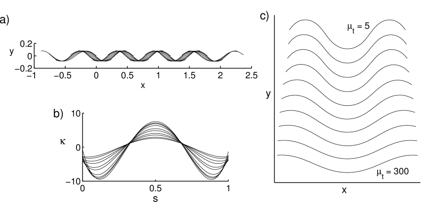
Figure 2: Numerical traveling-wave optima from AlbenSnake2013I for ten different $\mu_{t}\gg 1$. a) Snake trajectory over one period, from one snake optimization run for $\mu_{b}=1$ and $\mu_{t}=30$. b) Curvature versus arc length at the instant when a curvature maximum crosses the snake midpoint, for ten $\mu_{t}$ values: 5, 6, 7, 10, 20, 30, 60, 100, 200, and 300. c) Snake shapes corresponding to the curvatures in (b).

We now analytically determine the optimal snake motion in the limit of large $\mu_{t}$. Figure 2 shows a few numerical results from AlbenSnake2013I , which provide some intuition as we develop the analytical solution. In AlbenSnake2013I we show that for $\mu_{t}\gtrsim 6$, the numerically-computed optimal motions are always (retrograde) traveling waves, an example of which is shown in panel a for $\mu_{t}=30$. A sequence of snapshots of the snake is shown over a period of motion. The snake moves from left to right, and appears to follow a sinusoidal path, very similar to what has been observed biologically and studied numerically HuSh2012a . We have computed similar traveling-wave optima at a range of $\mu_{t}\gg 1$. In panel b we compare the curvatures from these optimal motions at a particular instant when a curvature maximum occurs at the snake midpoint, for ten different values of $\mu_{t}$: 5, 6, 7, 10, 20, 30, 60, 100, 200, and 300. The profiles are similar, but the amplitudes decay monotonically as $\mu_{t}$ increases. Panel c shows the ten snake shapes corresponding to the curvatures in panel b. Consistently, we see the decay of the traveling-wave amplitude as $\mu_{t}$ increases. With this picture from the numerics, we now proceed to derive the analyical solution in the asymptotic limit of large $\mu_{t}$.

We begin with the position of the snake in terms of its components:

$$\mathbf{X}(s,t)=(x(s,t),y(s,t)).$$ (18)

If $\mu_{t}$ is large, the snake moves more easily in the tangential direction than in the transverse direction. Furthermore, the most efficient curvature function will give motion mainly in the tangential direction, to avoid large work done against friction. We assume that the mean direction of motion is aligned with the $x$-axis, and that the deflections from the $x$-axis are small—that is, $|y|,|\partial_{t}y|,|\partial_{s}y|$ and higher derivatives are $O(\mu_{t}^{\alpha})$ for some negative $\alpha$. This has been observed in the numerical solutions, and makes intuitive sense. Small deflections allow the snake to move along a nearly straight path, which is more efficient than a more curved path, which requires more tangential motion (and work done against tangential friction) for a given forward motion, i.e. $d$.

We expand each of the terms in the force and torque balance equations in powers of $|y|$ and retain only the terms which are dominant at large $\mu_{t}$. We expand the cost of locomotion similarly, and find the dynamics which minimize it, in terms of $y(s,t)$.

We first expand $x(s,t)$. We decompose $x(s,t)$ into its $s$-average $\bar{x}$ and a zero-$s$-average remainder:

$$x(s,t)=\overline{x(s,t)}+-\int^{s}\cos{\theta(s^{\prime},t)}\,ds^{\prime}$$ (19)

where $-\int^{s}$ means the constant of integration is chosen so that the integrated function has zero $s$-average. Hence

$$\partial_{t}x(s,t)=\overline{\partial_{t}x(s,t)}+-\int^{s}-\partial_{t}\theta(s^{\prime},t)\sin{\theta(s^{\prime},t)}\,ds^{\prime}.$$ (20)

We denote the $s$-averaged horizontal velocity (the horizontal velocity of the snake center of mass) by

$$U(t)\equiv\overline{\partial_{t}x(s,t)}.$$ (21)

We expand the integrand in (20) in powers of $|y|$ and its derivatives:

$$-\partial_{t}\theta(s,t)\sin{\theta(s,t)}=-\partial_{st}y(s,t)\partial_{s}y(s,t)+O(|\partial_{s}y|^{4}).$$ (22)

The quartic remainder term in (22), $O(|\partial_{s}y|^{4})$, actually includes other quartic terms involving time derivatives of $\partial_{s}y$, but for brevity we use the assumption (which will be correct for our solution) that $|y|$ and all its derivatives are of the same order of smallness with respect to $\mu_{t}$. We define

$$h(s,t)=-\int^{s}-\partial_{s^{\prime}t}y(s^{\prime},t)\partial_{s^{\prime}}y(s^{\prime},t)ds^{\prime}$$ (23)

and with the small-deflection assumption, (20) becomes

$$\partial_{t}x(s,t)=U(t)+h(s,t)+O(|\partial_{s}y|^{4}),$$ (24)

and

$$\partial_{t}\mathbf{X}(s,t)=(U(t)+h(s,t),\partial_{t}y(s,t))+O(|\partial_{s}y|^{4}).$$ (25)

We will see that for a general class of shape dynamics near the optimum, $U(t)$ is $O$(1), i.e. of the same order as one snake length per actuation period, even in the limit of large $\mu_{t}$. $U$ is therefore the dominant term in (24) and (25). We use this assumption on $U$ to expand the velocity 2-norm:

$$\|\partial_{t}\mathbf{X}(s,t)\| =\sqrt{\partial_{t}x^{2}+\partial_{t}y^{2}}=U\left(1+\frac{h}{U}+\frac{1}{2}\frac{\partial_{t}y^{2}}{U^{2}}\right)+O(|y|^{4}).$$ (26)

In writing $O(|y|^{4})$ we have again lumped terms with four or more powers of $|y|$ and/or its $s$- and $t$-derivatives. Dividing (25) by (26), we obtain the expansion for the normalized velocity:

$$\widehat{\partial_{t}{\mathbf{X}}}(s,t)=\left({\begin{array}[]{c}1-\dfrac{1}{2}\dfrac{\partial_{t}y^{2}}{U^{2}}+O(|y|^{4})\vspace{0.3cm}\\ \dfrac{\partial_{t}y}{U}\left(1-\dfrac{h}{U}-\dfrac{1}{2}\dfrac{\partial_{t}y^{2}}{U^{2}}\right)+O(|y|^{5})\\ \end{array}}\right).$$ (27)

We next expand the unit tangent and normal vectors:

$$\hat{\mathbf{s}}=\left({\begin{array}[]{c}\partial_{s}x\\ \partial_{s}y\end{array}}\right)=\left({\begin{array}[]{c}\sqrt{1-\partial_{s}y^{2}}\\ \partial_{s}y\end{array}}\right) =\left({\begin{array}[]{c}1-\frac{1}{2}\partial_{s}y^{2}\\ \partial_{s}y\end{array}}\right)+O(|y|^{4}).$$ (34)

$$\hat{\mathbf{n}} =\left({\begin{array}[]{c}-\partial_{s}y\\ 1-\frac{1}{2}\partial_{s}y^{2}\end{array}}\right)+O(|y|^{4}).$$ (37)

Using (27) – (37),

$$\widehat{\partial_{t}{\mathbf{X}}}\cdot\hat{\mathbf{s}} =1-\frac{1}{2}\left(\partial_{s}y-\frac{\partial_{t}y}{U}\right)^{2}+O(|y|^{4}),$$ (38)

$$\widehat{\partial_{t}{\mathbf{X}}}\cdot\hat{\mathbf{n}} =\left(\frac{\partial_{t}y}{U}-\partial_{s}y\right)\left(1-\frac{1}{2}\frac{\partial_{t}y^{2}}{U^{2}}\right)+\frac{\partial_{t}y}{U}\left(-\frac{h}{U}-\frac{1}{2}\partial_{s}y^{2}\right)+O(|y|^{5}).$$ (39)

Using (38) and (39) we can write the force and torque balance equations (11)–(13) and the cost of locomotion $\eta$ in terms of $U$, $h$, and derivatives of $y$.

III.1 Traveling-wave optimum

We first expand $\eta$ and use it to argue that the optimal shape dynamics is approximately a traveling wave. This allows us to neglect certain terms, which simplifies the formulae for the rest of the analysis. If the power expended at time $t$ is $P(t)$, the cost of locomotion is

$$\eta =\int_{0}^{1}P(t)dt{\Bigg{/}}\int_{0}^{1}U(t)dt.$$ (40)

$$=\int_{0}^{1}U(t)\int_{0}^{1}\left[\left(\widehat{\partial_{t}{\mathbf{X}}}\cdot\hat{\mathbf{s}}\right)^{2}+\mu_{t}\left(\widehat{\partial_{t}{\mathbf{X}}}\cdot\hat{\mathbf{n}}\right)^{2}\right]\frac{\|\partial_{t}\mathbf{X}\|}{U(t)}\,ds\,dt{\Bigg{/}}\int_{0}^{1}U(t)\,dt.$$ (41)

In (41) we have assumed that the tangential motion of the snake is entirely forward, with no portion moving backward, so the coefficient in front of the tangential term is unity (i.e. $\mu_{f}$, rather than a term involving both $\mu_{f}$ and $\mu_{b}$). This assumption is not required but it simplifies the equations from this point onward and will be seen to be correct shortly. The numerator of (41) can be separated into a part involving tangential velocity and a part involving normal velocity with a factor of $\mu_{t}$. Using (26), (38), and (39), we can list the terms with the lowest powers of $y$ in each part:

$$\left(\widehat{\partial_{t}{\mathbf{X}}}\cdot\hat{\mathbf{s}}\right)^{2}\frac{\|\partial_{t}\mathbf{X}\|}{U(t)} =1+O(|y|^{2})$$ (42)

$$\mu_{t}\left(\widehat{\partial_{t}{\mathbf{X}}}\cdot\hat{\mathbf{n}}\right)^{2}\frac{\|\partial_{t}\mathbf{X}\|}{U(t)} =\mu_{t}\left(\partial_{s}y-\frac{\partial_{t}y}{U}\right)^{2}+O(\mu_{t}|y|^{4}).$$ (43)

The optimal shape dynamics is a $y(s,t)$ that minimizes $\eta$ subject to the constraints of force and torque balance. The leading-order term in (42) is 1, which is independent of the shape dynamics. At the next (quadratic) order in $y$, terms appear in both (42) and (43); only that in (43) is given explicitly. It is multiplied by $\mu_{t}$, so it appears to be dominant in the large $\mu_{t}$ limit. Thus, to a first approximation, minimizing $\eta$ is achieved by setting

$$\left(\partial_{s}y-\frac{\partial_{t}y}{U}\right)=0,$$ (44)

so a first guess for the solution is a traveling wave, i.e. a function of $s+Ut$ with $U$ constant. However, such a function does not satisfy the $x$-component of the force balance equation (11), which is:

$$\int\left[\left(\widehat{\partial_{t}{\mathbf{X}}}\cdot\hat{\mathbf{s}}\right)s_{x}+\mu_{t}\left(\widehat{\partial_{t}{\mathbf{X}}}\cdot\hat{\mathbf{n}}\right)n_{x}\right]\,ds=0.$$ (45)

Inserting (38) and (39) and retaining only the lowest powers in $y$ from each expression,

$$\int_{0}^{1}1+\mu_{t}\left(\partial_{s}y-\frac{\partial_{t}y}{U}\right)\partial_{s}y\;ds=0.$$ (46)

which cannot be satistied by a function of $s+Ut$. Physically, the first term (unity) in (46) represents the leading-order drag force on the body due to forward friction. For a function of $s+Ut$, in which the deflection wave speed equals the forward speed, the snake body moves purely tangentially (up to this order of expansion in $y$) along a fixed path on the ground, with no transverse forces to balance the drag from tangential frictional forces. Also, when a function of $s+Ut$ is inserted into (46) all factors of $U$ cancel out and $U$ is left undetermined. This is related to a more fundamental reason why posing the shape dynamics as a function of $s+Ut$ is invalid: the problem of solving for the snake dynamics given in section II is not then well-posed. In the well-posed problem we provide the snake curvature and curvature velocity versus time as inputs, and solve the force and torque balance equations to obtain the average translational and rotational velocities as outputs. Thus $U(t)$ is one of the three outputs (or unknowns) that is needed to solve the three equations.

Instead we pose the shape dynamics as

$$y(s,t)=g(s+U_{w}t),$$ (47)

which is a traveling wave with a prescribed wave speed $U_{w}$, different from $U$ in general. Since $y$ is periodic in $t$ with period 1, $g$ is periodic with a period of $U_{w}$. Inserting (47) into (46), we obtain an equation for $U$ in terms of $U_{w}$ and $g$:

$$1+\mu_{t}\left(1-\frac{U_{w}}{U}\right)\int_{0}^{1}g^{\prime}(s+U_{w}t)^{2}ds=0.$$ (48)

In (48), as $\mu_{t}\to\infty$, $(1-U_{w}/U)\to 0^{-}$. In the solution given by (47) and (48), the shape wave moves backwards along the snake at speed $U_{w}$, which propels the snake forward at a speed $U$, with $U$ slightly less than $U_{w}$. Therefore the snake slips transversely to itself, in the backward direction, which provides a forward thrust to balance the backward drag due to forward tangential friction. We refer to $(1-U_{w}/U)$ in (48), a measure of the amount of backward slipping of the snake, as the “slip.” In figure 2a, the snake slips transversely to itself, and backward (leftward), even as it moves rightward. Here the slip is fairly small because $\mu_{t}$ is 30, fairly large.

We now solve (48) for $(1-U_{w}/U)$ and insert the result into (41) to find $g$ and $U_{w}$ which minimize $\eta$. Using the lowest order expansions (42) and (43) with (48) we obtain:

$$\eta =\int_{0}^{1}P(t)dt{\Bigg{/}}\int_{0}^{1}U(t)dt.$$ (49)

$$=\int_{0}^{1}U(t)\int_{0}^{1}1+\mu_{t}\left(\partial_{s}y-\frac{\partial_{t}y}{U}\right)^{2}+O(|y|^{2},\mu_{t}|y|^{4})dsdt{\Bigg{/}}\int_{0}^{1}U(t)\,dt.$$ (50)

$$=1{\Bigg{/}}\int_{0}^{1}\cfrac{1}{1+\cfrac{1}{\mu_{t}\langle g^{\prime}(s+U_{w}t)^{2}\rangle+O(|g|^{2},\mu_{t}|g|^{4})}}\,dt.$$ (51)

where

$$\langle g^{\prime}(s+U_{w}t)^{2}\rangle\equiv\int_{0}^{1}g^{\prime}(s+U_{w}t)^{2}ds.$$ (52)

If we minimize (51) over possible $g$ for a given $\mu_{t}$, using only the terms in the expansion that are given explicitly, we find that $\eta$ tends to a minimum of 1 as the amplitude of $g$ diverges. However, in this limit our small-$y$ power series expansions are no longer valid. We therefore add the next-order terms in our expansions of $\eta$ and the $F_{x}$ equation and search again for an $\eta$-minimizer.

III.2 Optimal wave amplitude

We now expand to higher order the components of $\eta$, (42) and (43),

$$\left(\widehat{\partial_{t}{\mathbf{X}}}\cdot\hat{\mathbf{s}}\right)^{2}\frac{\|\partial_{t}\mathbf{X}\|}{U(t)} =1-\left(\partial_{s}y-\frac{\partial_{t}y}{U}\right)^{2}+\frac{h}{U}+\frac{1}{2}\frac{\partial_{t}y^{2}}{U^{2}}+O(|y|^{4})$$ (53)

$$\mu_{t}\left(\widehat{\partial_{t}{\mathbf{X}}}\cdot\hat{\mathbf{n}}\right)^{2}\frac{\|\partial_{t}\mathbf{X}\|}{U(t)} =\mu_{t}\left[\left(\frac{\partial_{t}y}{U}-\partial_{s}y\right)+\frac{\partial_{t}y}{U}\left(-\frac{h}{U}-\frac{1}{2}\partial_{s}y^{2}\right)\right]^{2}\left(1+O(|y|^{2})\right),$$ (54)

and equation (11),

$$\int 1+\mu_{t}\left(\partial_{s}y-\frac{\partial_{t}y}{U}+\frac{\partial_{t}y}{U}\left(\frac{h}{U}+\frac{1}{2}\partial_{s}y^{2}\right)\right)\partial_{s}y\;ds=0.$$ (55)

We again assume the traveling wave form of $y$ (47), and use this to evaluate $h$ given by (23) in terms of $g$:

$$h(s,t)=-\frac{U_{w}}{2}g^{\prime}(s+U_{w}t)^{2}+\frac{U_{w}}{2}\langle g^{\prime}(s+U_{w}t)^{2}\rangle.$$ (56)

Inserting the traveling-wave forms of $y$ (47) and $h$ (56) into (55) we obtain

$$1+\mu_{t}\left[\left(1-\frac{U_{w}}{U}\right)\langle g^{\prime}(s+U_{w}t)^{2}\rangle+\frac{1}{2}\langle g^{\prime}(s+U_{w}t)^{2}\rangle^{2}\right]=0.$$ (57)

To obtain (57) we’ve used the fact that the slip $(1-U_{w}/U)\to 0$ as $\mu_{t}\to\infty$, which will be verified subsequently. One can also proceed without this assumption, at the expense of a lengthier version of (57). We insert the traveling-wave forms of $y$ and $h$ into (53) and (54) to obtain $\eta$, again with the assumption that $(1-U_{w}/U)\to 0$ as $\mu_{t}\to\infty$ to simplify the result:

$$\eta=1+\int_{0}^{1}\frac{1}{2}\langle g^{\prime}(s+U_{w}t)^{2}\rangle+\mu_{t}\left(1-\frac{U_{w}}{U}+\frac{1}{2}\langle g^{\prime}(s+U_{w}t)^{2}\rangle\right)^{2}\langle g^{\prime}(s+U_{w}t)^{2}\rangle\;dt$$ (58)

Solving for the slip $(1-U_{w}/U)$ from (57) and inserting into (58), we obtain an improved version of (51):

$$\eta=1{\Bigg{/}}\int_{0}^{1}\cfrac{1}{1+\frac{1}{2}\langle g^{\prime}(s+U_{w}t)^{2}\rangle+\cfrac{1}{\mu_{t}\langle g^{\prime}(s+U_{w}t)^{2}\rangle}+O(|g|^{4},\mu_{t}|g|^{8})}\,dt.$$ (59)

(59) is a more accurate version of (51), with an additional term in the denominator of the integrand which penalizes large amplitudes for $g$. If we approximate $\langle g^{\prime}(s+U_{w}t)^{2}\rangle$ as constant in time, we obtain

$$\eta=1+\frac{1}{2}\langle g^{\prime 2}\rangle+\cfrac{1}{\mu_{t}\langle g^{\prime 2}\rangle}+O(|g|^{4},\mu_{t}|g|^{8}).$$ (60)

which is minimized for

$$\langle g^{\prime 2}\rangle^{1/2}=2^{1/4}\mu_{t}^{-1/4}.$$ (61)

Thus the RMS amplitude of the optimal $g$ should scale as $\mu_{t}^{-1/4}$. (61) represents a balance between competing effects. At smaller amplitudes, the forward component of normal friction is not large enough to balance the forward component of tangential friction, so the snake slips more, which reduces its forward motion and does more work in the normal direction. At larger amplitudes, as already noted, the snake’s path is more curved, which requires more work done against tangential friction for a given forward distance traveled. (61) is only a criterion for the amplitude of the motion. To obtain information about the shape of the optimal $g$, we now consider the balances of the $y$-component of the force and the torque.

III.3 Small-wavelength shapes

So far we have searched for the optimal shape dynamics in terms of $y(s,t)$, but in fact it is the curvature $\kappa(s,t)$ which is prescribed. We obtain $y(s,t)$ from the curvature by integrating twice in $s$:

$$y(s,t) =y(0,t)+\int_{0}^{s}\sin\theta(s^{\prime},t)ds^{\prime}$$ (62)

$$=y(0,t)+\int_{0}^{s}\theta(s^{\prime},t)ds^{\prime}+O(y^{3})$$ (63)

$$=y(0,t)+\int_{0}^{s}\left[\theta(0,t)+\int_{0}^{s^{\prime}}\kappa(s^{\prime\prime},t)ds^{\prime\prime}\right]ds^{\prime}+O(y^{3}).$$ (64)

$$=y(0,t)+\theta(0,t)s+\int_{0}^{s}\int_{0}^{s^{\prime}}\kappa(s^{\prime\prime},t)ds^{\prime\prime}ds^{\prime}+O(y^{3}).$$ (65)

$$\equiv Y(t)+sR(t)+k(s,t)+O(y^{3}).$$ (66)

where $Y$ and $R$ are defined for notational convenience. Prescribing the curvature is equivalent to prescribing $k(s,t)$. We set

$$k(s,t)=g(s+U_{w}t)$$ (67)

so we have the same form for $y$ as before, with an additional translation $Y(t)$ and rotation $R(t)$. $Y$ and $R$ are determined by the $y$-force and torque balance equations:

$$\int_{0}^{1}\left[\left(\widehat{\partial_{t}{\mathbf{X}}}\cdot\hat{\mathbf{s}}\right)s_{y}+\mu_{t}\left(\widehat{\partial_{t}{\mathbf{X}}}\cdot\hat{\mathbf{n}}\right)n_{y}\right]\,ds=0.$$ (68)

$$\int_{0}^{1}\left[\left(\widehat{\partial_{t}{\mathbf{X}}}\cdot\hat{\mathbf{s}}\right)(xs_{y}-ys_{x})+\mu_{t}\left(\widehat{\partial_{t}{\mathbf{X}}}\cdot\hat{\mathbf{n}}\right)(xn_{y}-yn_{x})\right]\,ds=0.$$ (69)

We expand these to leading order in $y$ and obtain

$$\int_{0}^{1}\partial_{s}y-\frac{\partial_{t}y}{U}+\frac{\partial_{t}y}{U}\left(\frac{h}{U}+\frac{1}{2}\partial_{s}y^{2}\right)\,ds=0.$$ (70)

$$\int_{0}^{1}s\left(\partial_{s}y-\frac{\partial_{t}y}{U}+\frac{\partial_{t}y}{U}\left(\frac{h}{U}+\frac{1}{2}\partial_{s}y^{2}\right)\right)\,ds=0.$$ (71)

We insert (66) with (67) into the three equations (55), (70), and (71) to solve for the three unknowns, $U$, $Y$, and $R$ in terms of $g$ and $U_{w}$. We obtain:

$$\int_{0}^{1}1+\mu_{t}\left[\left(-\frac{U_{w}}{U}+1+\frac{1}{2}\langle g^{\prime 2}\rangle\right)g^{\prime 2}+\left(-\frac{Y^{\prime}}{U}-\frac{R^{\prime}s}{U}+R\right)g^{\prime}\right]ds=0.$$ (72)

$$\int_{0}^{1}\left(-\frac{U_{w}}{U}+1+\frac{1}{2}\langle g^{\prime 2}\rangle\right)g^{\prime}-\frac{Y^{\prime}}{U}-\frac{R^{\prime}s}{U}+R\,ds=0.$$ (73)

$$\int_{0}^{1}s\left[\left(-\frac{U_{w}}{U}+1+\frac{1}{2}\langle g^{\prime 2}\rangle\right)g^{\prime}-\frac{Y^{\prime}}{U}-\frac{R^{\prime}s}{U}+R\right]\,ds=0.$$ (74)

We solve (73) and (74) for $Y$ and $R$ in terms of $U$:

$$\frac{Y^{\prime}}{U}-R =4B-6A$$ (75)

$$\frac{R^{\prime}}{U} =12A-6B$$ (76)

$$A \equiv\left(-\frac{U_{w}}{U}+1+\frac{1}{2}\langle g^{\prime 2}\rangle\right)\langle sg^{\prime}\rangle$$ (77)

$$B \equiv\left(-\frac{U_{w}}{U}+1+\frac{1}{2}\langle g^{\prime 2}\rangle\right)\langle g^{\prime}\rangle$$ (78)

We then solve (72) for $U$ in terms of $g$:

$$\frac{U_{w}}{U}=1+\frac{1}{2}\langle g^{\prime 2}\rangle+\frac{1}{\mu_{t}\left(\langle g^{\prime 2}\rangle-\langle g^{\prime}\rangle^{2}-3\left(\langle g^{\prime}\rangle-2\langle sg^{\prime}\rangle\right)^{2}\right)}.$$ (79)

We now form $\eta$, (41) with terms given by (53) and (54), using the updated from of $y$ ((66) with (67)) and (79). We obtain a more correct version of (59):

$$\eta=1{\Bigg{/}}\int_{0}^{1}\cfrac{1}{1+\frac{1}{2}\langle g^{\prime 2}\rangle+\cfrac{1}{\mu_{t}\left(\langle g^{\prime 2}\rangle-\langle g^{\prime}\rangle^{2}-3\left(\langle g^{\prime}\rangle-2\langle sg^{\prime}\rangle\right)^{2}\right)}+O(|g|^{4},\mu_{t}|g|^{8})}\,dt.$$ (80)

We can find $\eta$-minimizing $g$ in a few steps. First, let $\{L_{k}\}$ be the family of orthonormal polynomials with unit weight on $[0,1]$ (essentially the Legendre polynomials):

$$\int_{0}^{1}L_{i}L_{j}\,ds=\delta_{ij}\quad;\quad L_{0}\equiv 1\;,\;L_{1}=\sqrt{12}(s-1/2)\;,\ \ldots.$$ (81)

At a fixed time $t$ we expand $g^{\prime}$ in the basis of the $L_{k}$:

$$g^{\prime}(s+U_{w}t)=\sum_{k=0}^{\infty}c_{k}(t)L_{k}(s).$$ (82)

Then we have:

$$\langle g^{\prime 2}\rangle =\sum_{k=0}^{\infty}c_{k}(t)^{2},$$ (83)

$$\langle g^{\prime}\rangle^{2} =c_{0}(t)^{2},$$ (84)

$$3\left(\langle g^{\prime}\rangle-2\langle sg^{\prime}\rangle\right)^{2} =\langle L_{1}g^{\prime}\rangle^{2}=c_{1}(t)^{2}.$$ (85)

Inserting into (80), $\eta$ becomes

$$\eta=1{\Bigg{/}}\int_{0}^{1}\cfrac{1}{1+\frac{1}{2}\left(c_{0}(t)^{2}+c_{1}(t)^{2}+\sum_{k=2}^{\infty}c_{k}(t)^{2}\right)+\cfrac{1}{\mu_{t}\left(\sum_{k=2}^{\infty}c_{k}(t)^{2}\right)}+O(|g|^{4},\mu_{t}|g|^{8})}\,dt.$$ (86)

The denominator of the integrand in (86) is minimized when

$$c_{0}(t)=0\;;\;c_{1}(t)=0\;;\;\sum_{k=2}^{\infty}c_{k}(t)^{2}=\sqrt{2}\mu_{t}^{-1/2}.$$ (87)

The function $g(s+U_{w}t)$ that minimizes $\eta$ is that for which (87) holds for all $t$. Then the integral in (86) is maximized, so $\eta$ is minimized. Recall that $g$ is a periodic function with period $U_{w}$. The relations (87) hold for any such $g$ in the limit that $U_{w}\to 0$, as long as $g$ is normalized appropriately. Define

$$A\equiv\left(\frac{1}{U_{w}}\int_{0}^{U_{w}}g^{\prime}(x)^{2}dx\right)^{1/2}.$$ (88)

Then

$$\int_{0}^{1}g^{\prime}(s+U_{w}t)^{2}ds =A^{2}+O(U_{w})$$ (89)

$$\int_{0}^{1}g^{\prime}(s+U_{w}t)ds =O(U_{w})$$ (90)

$$\int_{0}^{1}sg^{\prime}(s+U_{w}t)ds =O(U_{w}).$$ (91)

(89) – (91) are fairly straightforward to show, and we show them in Appendix A for completeness. If (89) – (91) hold, then in the limit that $U_{w}\to 0$, (87) holds with $A=2^{1/4}\mu_{t}^{-1/4}$, by (83) – (85). A physical interpretation of the small-wavelength limit is that the net vertical force and torque on the snake due to the traveling wave alone ($g$) become zero in this limit, so no additional heaving motion ($Y$) or rotation ($R$) are needed, and thus the additional work associated with these motions is avoided. Similar “recoil” conditions were proposed as kinematic constraints in the context of fish swimming lighthill1975mathematica . We also note two other scaling laws. For a given $g\sim\mu_{t}^{-1/4}$, by (79) the slip $(1-U_{w}/U)\sim\mu_{t}^{-1/2}$ and by (75)–(78), $Y,R\sim\mu_{t}^{-3/4}$.

III.4 Optimal cost of locomotion and comparison with numerics

To obtain an $\eta$-minimizing function $g^{*}$, let $g$ be any periodic function with period $U_{w}$. Define

$$g^{*}(s+U_{w}t)\equiv\frac{2^{1/4}\mu_{t}^{-1/4}}{A}g(s+U_{w}t)$$ (92)

where $A$ is given in (88). Then in the limit $U_{w}\to 0$,

$$\eta(g^{*})\to 1+\sqrt{2}\mu_{t}^{-1/2}+O(\mu_{t}^{-1}),$$ (93)

by the estimate in (80). Thus the optimal traveling wave motions become more efficient as $\mu_{t}\to\infty$, which agrees with the numerical solutions in AlbenSnake2013I . The numerically-determined optima in figure 2 do not have small wavelengths, due to the finite number of modes used. This is explained further in the Supplementary Material of AlbenSnake2013I .

Figure 3: The $\mu_{t}$-scalings of the numerical traveling-wave optima from figure 2 and AlbenSnake2013I . (a) The cost of locomotion $\eta$ minus unity, on a log scale, for the numerical optima (squares) of AlbenSnake2013I together with $\eta-1$ for the analytical optimum (solid line). (b) The curvature from figure 2b rescaled by $\mu_{t}^{1/4}$. (c) The deflection from figure 2c rescaled by $\mu_{t}^{1/4}$.

We compare the numerically-found optima to the theoretical results in figure 3. Here we take the plots of figure 2 and transform them according to the theory. In figure 3a we plot $\eta-1$ versus $\mu_{t}$ for the numerical solutions (squares) from AlbenSnake2013I , along with the small-$U_{w}$ theoretical result (solid line), which is given by (93). The numerics follow the same scaling as the theory, but with a consistent upward shift. Some degree of upward shift is expected from the finite-mode truncation in the numerical computation, which makes the numerical result underperform the analytical result, as explained in AlbenSnake2013I . The circle shows the efficiency for a curvature function with a higher wavelength than those which could be represented in the numerical optimization, and its distance from the solid line is $O(\mu_{t}^{-1})$, of the order of the next term in the asymptotic expansion of $\eta-1$.

Figure 3b shows the curvature, rescaled by $\mu_{t}^{1/4}$ to give a collapse according to (61). The data collapse well compared to the unscaled data in figure 2b. Figure 3c shows the body shapes from figure 2c with the vertical coordinate rescaled, and the shapes plotted with all centers of mass located at the origin. We again find a good collapse, consistent with the curvature collapse.

IV Conclusion

We have studied the optimization of planar snake motions for efficiency, using a fairly simple model for the motion of snakes using friction. When the coefficient of transverse friction is large, our analysis shows that a traveling-wave motion of small amplitude is optimal. The amplitude tends to zero as the transverse friction coefficient tends to infinity, scaling as the transverse friction coefficient to the -1/4 power, and the efficiency tends to unity in this limit. The corresponding power is that for a straight snake towed forward.

In AlbenSnake2013I we were able to compute many optimal motions at moderate and small $\mu_{t}$ also. Those found at small $\mu_{t}$ also corresponded to traveling waves (direct now, not retrograde), and at zero $\mu_{t}$, a simple triangular-wave solution was found with optimal efficiency. It remains to determine optimal motions with small but nonzero $\mu_{t}$ analytically. At moderate $\mu_{t}$, a region of standing-wave or ratcheting motions was found. It may be possible to compute some of these motions analytically using a set of assumptions specialized to the moderate-$\mu_{t}$ regime.

Appendix A Small-wavelength integrals

To show (89) – (91), we first note that since $g$ is periodic, $g^{\prime}$ is periodic with zero average over a period. To show (89), we decompose the integral in (89) into two intervals:

$$\int_{0}^{1}g^{\prime}(s+U_{w}t)^{2}ds=\int_{0}^{U_{w}\lfloor{1/U_{w}}\rfloor}g^{\prime}(s+U_{w}t)^{2}ds+\int_{U_{w}\lfloor{1/U_{w}}\rfloor}^{1}g^{\prime}(s+U_{w}t)^{2}ds.$$ (94)

The first integral on the right of (94) is over an integral number of periods of $g^{\prime 2}$, and is thus $\lfloor{1/U_{w}}\rfloor U_{w}A^{2}=A^{2}+O(U_{w})$. The second integral is over an interval of length $<U_{w}$, and is thus $O(U_{w})$, which shows (89). To show (90), we use (94) again but with $g^{\prime}$ in place of $g^{\prime 2}$:

$$\int_{0}^{1}g^{\prime}(s+U_{w}t)ds=\int_{0}^{U_{w}\lfloor{1/U_{w}}\rfloor}g^{\prime}(s+U_{w}t)ds+\int_{U_{w}\lfloor{1/U_{w}}\rfloor}^{1}g^{\prime}(s+U_{w}t)ds.$$ (95)

The first integral on the right of (95) is over an integral number of periods of $g^{\prime}$, and is thus zero. The second integral is over an interval of length $<U_{w}$, and is thus $O(U_{w})$. To show (91), we decompose the integral into three parts:

$$\int_{0}^{1}s g^{\prime}(s+U_{w}t)ds=\int_{0}^{U_{w}\lfloor{1/U_{w}}\rfloor}{U_{w}\lfloor{s/U_{w}}\rfloor}g^{\prime}(s+U_{w}t)ds$$

$$+\int_{0}^{U_{w}\lfloor{1/U_{w}}\rfloor}(s-{U_{w}\lfloor{s/U_{w}}\rfloor})g^{\prime}(s+U_{w}t)ds+\int_{U_{w}\lfloor{1/U_{w}}\rfloor}^{1}sg^{\prime}(s+U_{w}t)ds.$$ (96)

The first integral on the right of (96) substitutes a constant approximation to $s$ on each subinterval of period length. It is identically zero since $g^{\prime}$ has mean zero. The second integral is the error in the constant approximation to $s$, $O(U_{w})$ on each subinterval, of which there are $O(1/U_{w})$, each of length $U_{w}$. Thus the second integral is $O(U_{w})$. The third integral is also $O(U_{w})$, as explained for (94) and (95), so (91) holds.

References

• [1] S Alben. Optimizing snake locomotion in the plane. I. Computations. submitted, 2013.
• [2] Z V Guo and L Mahadevan. Limbless undulatory propulsion on land. Proceedings of the National Academy of Sciences, 105(9):3179, 2008.
• [3] D L Hu, J Nirody, T Scott, and M J Shelley. The mechanics of slithering locomotion. Proceedings of the National Academy of Sciences, 106(25):10081, 2009.
• [4] R L Hatton and H Choset. Generating gaits for snake robots: annealed chain fitting and keyframe wave extraction. Autonomous Robots, 28(3):271–281, 2010.
• [5] Hamidreza Marvi and David L Hu. Friction enhancement in concertina locomotion of snakes. Journal of The Royal Society Interface, 9(76):3067–3080, 2012.
• [6] D L Hu and M Shelley. Slithering Locomotion. Natural Locomotion in Fluids and on Surfaces, pages 117–135, 2012.
• [7] J Gray and HW Lissmann. The kinetics of locomotion of the grass-snake. Journal of Experimental Biology, 26(4):354–367, 1950.
• [8] Michael H Dickinson, Claire T Farley, Robert J Full, MAR Koehl, Rodger Kram, and Steven Lehman. How animals move: an integrative view. Science, 288(5463):100–106, 2000.
• [9] L E Becker, S A Koehler, and H A Stone. On self-propulsion of micro-machines at low Reynolds number: Purcell’s three-link swimmer. Journal of Fluid Mechanics, 490(1):15–35, 2003.
• [10] J E Avron, O Gat, and O Kenneth. Optimal swimming at low Reynolds numbers. Physical Review Letters, 93(18):186001, 2004.
• [11] D Tam and A E Hosoi. Optimal stroke patterns for Purcell’s three-link swimmer. Physical Review Letters, 98(6):68105, 2007.
• [12] Henry C Fu, Thomas R Powers, and Charles W Wolgemuth. Theory of swimming filaments in viscoelastic media. Physical Review Letters, 99(25):258101, 2007.
• [13] Saverio E Spagnolie and Eric Lauga. The optimal elastic flagellum. Physics of Fluids, 22:031901, 2010.
• [14] Darren Crowdy, Sungyon Lee, Ophir Samson, Eric Lauga, and AE Hosoi. A two-dimensional model of low-Reynolds number swimming beneath a free surface. Journal of Fluid Mechanics, 681:24–47, 2011.
• [15] James Lighthill. Mathematical Biofluiddynamics. SIAM, 1975.
• [16] Stephen Childress. Mechanics of swimming and flying. Cambridge University Press, 1981.
• [17] JA Sparenberg. Hydrodynamic Propulsion and Its Optimization:(Analytic Theory), volume 27. Kluwer Academic Pub, 1994.
• [18] S. Alben. Passive and active bodies in vortex-street wakes. Journal of Fluid Mechanics, 642:95–125, 2009.
• [19] Sébastien Michelin and Stefan G Llewellyn Smith. Resonance and propulsion performance of a heaving flexible wing. Physics of Fluids, 21:071902, 2009.
• [20] J. Peng and S. Alben. Effects of shape and stroke parameters on the propulsion performance of an axisymmetric swimmer. Bioinspiration and Biomimetics, 7:016012, 2012.
• [21] F Jing and S Alben. Optimization of two- and three-link snake-like locomotion. Physical Review E, 87(2):022711, 2013.
• [22] S Hirose. Biologically Inspired Robots: Snake-Like Locomotors and Manipulators. Oxford University Press, 1993.
• [23] James K Hopkins, Brent W Spranklin, and Satyandra K Gupta. A survey of snake-inspired robot designs. Bioinspiration & Biomimetics, 4(2):021001, 2009.
• [24] Bo NJ Persson. Sliding Friction: Physical Principles and Applications, volume 1. Springer, 2000.
• [25] RG Cox. The motion of long slender bodies in a viscous fluid. Part 1. General theory. Journal of Fluid Mechanics, 44(04):791–810, 1970.