Coexistence of spin-triplet superconductivity with magnetism within a single mechanism for orbitally degenerate correlated electrons: Statistically-consistent Gutzwiller approximation.

Abstract

An orbitally degenerate two-band Hubbard model is analyzed with inclusion of the Hund’s rule induced spin-triplet paired states and their coexistence with magnetic ordering. The so-called statistically consistent Gutzwiller approximation (SGA) has been applied to the case of a square lattice. The superconducting gaps, the magnetic moment, and the free energy are analyzed as a function of the Hund’s rule coupling strength and the band filling. Also, the influence of the intersite hybridization on the stability of paired phases is discussed. In order to examine the effect of correlations the results are compared with those calculated earlier within the Hartree-Fock (HF) approximation combined with the Bardeen-Cooper-Schrieffer (BCS) approach. Significant differences between the two used methods (HF+BCS vs. SGA+real-space pairing) appear in the stability regions of the considered phases. Our results supplement the analysis of this canonical model used widely in the discussions of pure magnetic phases with the detailed elaboration of the stability of the spin-triplet superconducting states and the coexistent magnetic-superconducting states. At the end, we briefly discuss qualitatively the factors that need to be included for a detailed quantitative comparison with the corresponding experimental results.

1 Introduction

The question of coexistence of magnetism and superconductivity appears very often in correlated electron systems. In this context, both the spin-singlet and the spin-triplet paired states should be considered. A general motivation for considering here the spin-triplet pairing is provided by the discoveries of superconductivity in Sr₂RuO₄ [1, 2], UGe₂ [3, 4], URhGe [5], UIr [6], and UCoGe [7, 8, 9]. In the last four compounds, superconductivity indeed coexists with ferromagnetism. Moreover, for both, the spin-singlet high-temperature superconductors and the heavy-fermion systems, the antiferromagnetism and the superconductivity can have the same origin. Hence, it is natural to ask whether ferromagnetism and spin-triplet superconductivity also have the same origin in the itinerant uranium ferromagnets. A related and a very nontrivial question is concerned with the coexistence of antiferromagnetism with triplet superconducting state as in UNi₂Al₃ [10, 11, 12] and UPt₃ [13, 14].

It has been argued earlier [15, 17, 18, 19] that for the case of indistinguishable fermions, the intra-atomic Hund’s rule exchange can lead in a natural manner to the coexistence of spin-triplet superconductivity with magnetic ordering - ferromagnetism or antiferromagnetism in the simplest situations. This idea has been elaborated subsequently by us [20, 21, 22] by means of the combined Hartree-Fock(HF)-Bardeen-Cooper-Shrieffer(BCS) approach. In particular, the phase diagrams have been determined which contain regions of stability of the pure superconducting phase of type A (i.e., the equal-spin-paired phase), as well as superconductivity coexisting with either ferromagnetism or antiferromagnetism.

The HF approximation, as a rule, overestimates the stability of phases with a broken symmetry. Therefore, in this work, we apply the Gutzwiller approximation for the same selection of phases in order to examine explicitly the effects of interelectronic correlations. The extension of the Gutzwiller method to the multi-band case [23, 24, 25] provides us with the so-called renormalization factors for our degenerate two-band models. With these factors we construct an effective Hamiltonian by means of the statistically consistent Gutzwiller approximation, SGA, in which additional constraints are added to the standard Gutzwiller approximation (GA) and with the incorporation of which the single-particle state has been determined (see [26, 27, 28, 29] for exemplary applications of the SGA method). The detailed phase diagram and the corresponding order parameters are determined as functions of the microscopic parameters such as the band filling, $n$, the Hund’s rule exchange integral, $J$, and the Hubbard interaction parameters, $U$ and $U^{\prime}$. The obtained results are compared with those coming out from the Hartree-Fock approximation. In this manner, the paper extends the discussion of itinerant magnetism within the canonical (extended Hubbard) model, appropriate for this purpose, to the analysis of pure and coexisting superconducting-magnetic states within a single unified approach. Additionally, at the end, we dwell briefly on the applicability of our original concepts to more realistic systems. It should be noted that theoretical investigations regarding the spin-triplet pairing have been performed recently also for other systems [30, 31, 32, 33, 34, 35].

The paper is composed as follows. In Sec. II we provide the principal aspects of real-space spin-triplet pairing induced by the Hund’s rule coupling, and introduce the band-renormalization factors for our two-band model. Furthermore, in subsections A and B of Sec. II we explain how the effective Hamiltonian is constructed, according to the statistically consistent Gutzwiller approximation, for all the phases considered in this work. In Sec. III we discuss the phase diagram, and the principal order parameters in the considered phases, whereas Sec. IV contains the concluding remarks and outlook concerning future investigations to make the approach applicable to real systems.

2 Model and method

We consider the extended orbitally-degenerate Hubbard Hamiltonian, which has the form

$$\begin{split}\hat{H}&=\sum_{ij(i\neq j)ll^{\prime}\sigma}t^{ll^{\prime}}_{ij}\hat{c}_{il\sigma}^{{\dagger}}\hat{c}_{jl^{\prime}\sigma}+(U^{\prime}+J)\sum_{i}\hat{n}_{i1}\hat{n}_{i2}\\ &+U\sum_{il}\hat{n}_{il\uparrow}\hat{n}_{il\downarrow}-J\sum_{ill^{\prime}(l\neq l^{\prime})}\bigg{(}\mathbf{\hat{S}}_{il}\cdotp\mathbf{\hat{S}}_{il^{\prime}}+\frac{3}{4}\hat{n}_{il}\hat{n}_{il^{\prime}}\bigg{)}\\ &=\hat{H}^{0}+\hat{H}^{at}\;,\end{split}$$ (1)

where $l=1,2$ label the orbitals and the first term describes electron hopping between atomic sites $i$ and $j$. For $l\neq l^{\prime}$ this term represents electron hopping with change of the orbital (i.e., hybridization in momentum space). The next two terms describe the Coulomb interactions between electrons on the same atomic site. However the second term contains also the contribution, originating from the exchange interaction ($J$). The last term expresses the Hund’s rule i.e., the ferromagnetic exchange between electrons localized on the same site, but on different orbitals. This term contributes to magnetic coupling and is responsible for the spin-triplet pairing leading to magnetic ordering, superconductivity and coexistent magnetic-superconducting phases. In the Hamiltonian (1), we have disregarded the pair hopping term $(J/2)\sum_{l\neq l^{\prime}}\hat{c}^{\dagger}_{il\uparrow}\hat{c}^{\dagger}_{il\downarrow}\hat{c}_{il^{\prime}\downarrow}\hat{c}_{il^{\prime}\uparrow}$ because it hardly influences the ordered phases which we analyze in this work. In our variational method we assume that the correlated state $|\Psi_{G}\rangle$ of the system can be expressed in the following manner

$$|\Psi_{G}\rangle=\hat{P}_{G}|\Psi_{0}\rangle\;,$$ (2)

where $|\Psi_{0}\rangle$ is the normalized non-correlated state to be determined later and $\hat{P}_{G}$ is the Gutzwiller correlator selected in the following form

$$\hat{P}_{G}=\prod_{i}\hat{P}_{G|i}=\prod_{i}\sum_{I,I^{\prime}}\lambda^{(i)}_{I,I^{\prime}}|I\rangle_{ii}\langle I^{\prime}|\;.$$ (3)

Here, $\lambda^{(i)}_{I,I^{\prime}}$ are the variational parameters, which are assumed to be real. In the two-band situation the local basis consists of 16 states (see Table 4), which are defined as follows

$$|I\rangle_{i}=\hat{C}^{\dagger}_{i,I}|0\rangle_{i}\equiv\prod_{\gamma\in I}\hat{c}_{i\gamma}^{\dagger}|0\rangle_{i}=\hat{c}^{\dagger}_{i\gamma_{1}}...\hat{c}^{\dagger}_{i{\gamma}_{|I|}}|0\rangle_{i}\;,$$ (4)

where $\gamma=1,2,3,4$ labels the four spin-orbital states (in the $l\sigma$ notation: $1\uparrow,1\downarrow,2\uparrow,2\downarrow$, respectively) and $|I|$ is the number of electrons in the local state $|I\rangle$. In general, an index $I$ can be interpreted as a set in the usual mathematical sense. The creation operators in (4) are placed in ascending order, i.e., $\gamma_{1}<...<\gamma_{|I|}$. In an analogous manner, one can define the product of annihilation operators

$$\hat{C}_{i,I}=\prod_{\gamma\in I}\hat{c}_{i\gamma}=\hat{c}_{i\gamma_{1}}...\hat{c}_{i\gamma_{|I|}}\;,$$ (5)

which are placed in descending order $\gamma_{1}>...>\gamma_{|I|}$.

Table 1: The local basis consisting of 16 configurations containing $N_{e}=0,...,4$ electrons, which are enumerated as shown below.

$|0,0\rangle$	1	$|0,\downarrow\rangle$	5	$|\downarrow,\downarrow\rangle$	9	$|\uparrow\downarrow,\uparrow\rangle$	13
$|\uparrow,0\rangle$	2	$|\uparrow\downarrow,0\rangle$	6	$|\uparrow,\downarrow\rangle$	10	$|\downarrow,\uparrow\downarrow\rangle$	14
$|0,\uparrow\rangle$	3	$|0,\uparrow\downarrow\rangle$	7	$|\downarrow,\uparrow\rangle$	11	$|\uparrow\downarrow,\downarrow\rangle$	15
$|\downarrow,0\rangle$	4	$|\uparrow,\uparrow\rangle$	8	$|\uparrow,\uparrow\downarrow\rangle$	12	$|\uparrow\downarrow,\uparrow\downarrow\rangle$	16

The operator $|I\rangle_{ii}\langle I^{\prime}|$ can be expressed in terms of $\hat{C}^{\dagger}_{I}$ and $\hat{C}_{I}$ in the following manner

$$\hat{m}_{I,I^{\prime}|i}\equiv|I\rangle_{ii}\langle I^{\prime}|=\hat{C}^{\dagger}_{i,I}\hat{C}_{i,I^{\prime}}\hat{n}^{h}_{I\cup I^{\prime}|i}\;,$$ (6)

where

$$\hat{n}^{h}_{I\cup I^{\prime}|i}=\prod_{\gamma\in\overline{I\cup I^{\prime}}}(1-\hat{n}_{i\gamma})\;.$$ (7)

In the subsequent discussion, we write expectation values with respect to $|\Psi_{0}\rangle$ as

$$\langle\hat{O}\rangle_{0}=\langle\Psi_{0}|\hat{O}|\Psi_{0}\rangle\;,$$ (8)

while the expectation values with respect to $|\Psi_{G}\rangle$ will be denoted by

$$\langle\hat{O}\rangle_{G}=\frac{\langle\Psi_{G}|\hat{O}|\Psi_{G}\rangle}{\langle\Psi_{G}|\Psi_{G}\rangle}\;.$$ (9)

The most important step within the Gutzwiller approach is to derive the formula for the expectation value of the Hamiltonian $\hat{K}=\hat{H}-\mu\hat{N}$ with respect to $|\Psi_{G}\rangle$. This can be done in the limit of infinite dimensions by a diagrammatic approach [25] which uses the variational analog of Feynmann diagrams. By applying this method to the interaction part of the Hamiltonian (1), which is completely of intra-site character, one obtains

$$\langle\hat{H}^{at}\rangle_{G}=L\sum_{I_{1},I_{4}}\bar{E}_{I_{1},I_{4}}\langle\hat{m}_{I_{1},I_{4}}\rangle_{0}\;,$$ (10)

where

$$\bar{E}_{I_{1},I_{4}}=\sum_{I_{2},I_{3}}\lambda_{I_{1},I_{2}}\lambda_{I_{3},I_{4}}\langle I_{2}|\hat{H}^{at}|I_{3}\rangle\;,$$ (11)

and $L$ is the number of atomic sites. In (10) we have assumed that our system is homogeneous. Note that, with the use of Wick’s theorem, the purely local expectation values $\langle\hat{m}_{I_{1},I_{4}}\rangle_{0}$ can be expressed in terms of the local single-particle density matrix elements $\langle\hat{c}^{\alpha}_{i\gamma}\hat{c}^{\alpha^{\prime}}_{i\gamma^{\prime}}\rangle_{0}$. Here, $\hat{c}^{\alpha}_{i\gamma}$ are either creation or annihilation operators.

The expectation value of the single-particle part in the Hamiltonian (1) can be cast to the form

$$\langle\hat{H^{0}}\rangle_{G}=\sum_{ij(i\neq j)}\sum_{\gamma\gamma^{\prime}\tilde{\gamma}\tilde{\gamma}^{\prime}}t^{\gamma\gamma^{\prime}}_{ij}\big{(}q_{\gamma\tilde{\gamma}}q_{\gamma^{\prime}\tilde{\gamma}^{\prime}}-\bar{q}_{\gamma\tilde{\gamma}}\bar{q}_{\gamma^{\prime}\tilde{\gamma}^{\prime}}\big{)}\langle\hat{c}^{\dagger}_{i,\tilde{\gamma}}\hat{c}_{j,\tilde{\gamma}^{\prime}}\rangle_{0}$$ (12)

where we have assumed that the renormalization factors $q$ and $\bar{q}$ are real numbers and $t^{\gamma\gamma^{\prime}}=t^{\gamma^{\prime}\gamma}$. Moreover, in the equation above we have neglected the part containing the inter-site pairing terms $\langle\hat{c}^{\dagger}_{i,\gamma}\hat{c}^{\dagger}_{j,\gamma^{\prime}}\rangle_{0}$ and $\langle\hat{c}_{i,\gamma}\hat{c}_{j,\gamma^{\prime}}\rangle_{0}$ as we are going to concentrate on the Hund’s rule induced intra-site spin-triplet paired states. The inter-site pairing amplitudes are much smaller than the intra-site terms, in the considered model. The renormalization factors, introduced in (12), have the form

$$q_{\gamma\tilde{\gamma}}=\sum_{I(\tilde{\gamma}\notin I)}\bigg{[}\sum_{I^{\prime}}\mbox{fsgn}(\tilde{\gamma},I)m^{0(\tilde{\gamma})}_{I,I^{\prime}}c^{*}_{I\cup\tilde{\gamma},I^{\prime}|\gamma}+\sum_{I^{\prime}(\tilde{\gamma}\notin I^{\prime})}\mbox{fsgn}(\tilde{\gamma},I)m^{0}_{I^{\prime},I\cup\tilde{\gamma}}c^{*}_{I^{\prime},I|\gamma}\bigg{]}\;,$$ (13)

where $m^{0}_{I,I^{\prime}}=\langle\hat{m}_{I,I^{\prime}}\rangle_{0}$ and $m^{0(\tilde{\gamma})}_{I,I^{\prime}}=\langle\hat{m}^{(\tilde{\gamma})}_{I,I^{\prime}}\rangle_{0}$. Here we have introduced the operator

$$\hat{m}^{(\gamma)}_{I,I^{\prime}}=\hat{C}^{\dagger}_{i,I}\hat{C}_{i,I^{\prime}}\hat{n}^{h}_{I\cup I^{\prime}\cup\gamma|i}\;.$$ (14)

The parameters $c^{*}_{I_{1},I_{2}|\gamma}$ in (13) are defined as

$$c^{*}_{I_{1},I_{2}|\gamma}=\sum_{I(\gamma\notin I)}\mbox{fsgn}(\gamma,I)\lambda_{I_{1},I\cup\gamma}\lambda_{I,I_{2}}\;,$$ (15)

where we introduced the fermionic sign function

$$\mbox{fsgn}(\gamma,I)\equiv\langle I\cup\gamma|\hat{c}^{\dagger}_{\gamma}|I\rangle\;.$$ (16)

The renormalization factors $\bar{q}_{\gamma\tilde{\gamma}}$ have to be included in (12), when there are nonzero gap parameters ($\langle\hat{c}^{\alpha}\hat{c}^{\alpha}\rangle_{0}\neq 0$) in $|\Psi_{0}\rangle$, which is the case considered here. The form of $\bar{q}_{\gamma\tilde{\gamma}}$ is as follows

$$\bar{q}_{\gamma\tilde{\gamma}}=\sum_{I(\tilde{\gamma}\notin I)}\bigg{[}\sum_{I^{\prime}}\mbox{fsgn}(\tilde{\gamma},I)m^{0(\tilde{\gamma})}_{I^{\prime},I}c^{*}_{I^{\prime},I\cup\tilde{\gamma}|\gamma}+\sum_{I^{\prime}(\tilde{\gamma}\notin I^{\prime})}\mbox{fsgn}(\tilde{\gamma},I)m^{0}_{I\cup\tilde{\gamma},I^{\prime}}c^{*}_{I,I^{\prime}|\gamma}\bigg{]}\;.$$ (17)

The remaining part of $\langle\hat{K}\rangle_{G}$ that has to be derived is the expectation value $\langle\hat{N}\rangle_{G}$. Also in this case, the diagrammatic evaluation in infinite dimensions gives the proper formula,

$$\langle\hat{N}\rangle_{G}=\sum_{i\gamma}\langle\hat{n}_{i\gamma}\rangle_{G}\;,$$ (18)

where

$$\langle\hat{n}_{i\gamma}\rangle_{G}=\sum_{I_{1},I_{4}}N^{\gamma}_{I_{1},I_{4}}m^{0}_{I_{1},I_{4}}\;,$$ (19)

and

$$N^{\gamma}_{I_{1},I_{4}}=\sum_{I(\gamma\notin I)}\lambda_{I_{1},I\cup\gamma}\lambda_{I\cup\gamma,I_{4}}\;.$$ (20)

The pairing densities in the correlated state that are going to be useful in the subsequent discussion can be expressed in the following way

$$\langle\hat{c}_{i\gamma}\hat{c}_{i\gamma^{\prime}}\rangle_{G}=\sum_{I_{1},I_{4}}S^{\gamma\gamma^{\prime}}_{I_{1},I_{4}}m^{0}_{I_{1},I_{4}}\;,$$ (21)

where

$$S^{\gamma\gamma^{\prime}}_{I_{1},I_{4}}=\sum_{I(\gamma\gamma^{\prime}\notin I)}\lambda_{I_{1},I}\lambda_{I\cup(\gamma\gamma^{\prime}),I_{4}}\mbox{fsgn}(\gamma,I)\mbox{fsgn}(\gamma^{\prime},I)\mbox{fsgn}(\gamma^{\prime},\gamma)\;.$$ (22)

Using (10), (12), and (18) one can express $\langle\hat{K}\rangle_{G}$ in terms of the variational parameters $\lambda_{I,I^{\prime}}$, local and non-local single particle density matrix elements ,$\langle\hat{c}^{\alpha}_{i\gamma}\hat{c}^{\alpha^{\prime}}_{i\gamma^{\prime}}\rangle_{0}$, $\langle\hat{c}^{\dagger}_{i,\gamma}\hat{c}_{j,\gamma^{\prime}}\rangle_{0}$, and the matrix elements of the atomic part of the atomic Hamiltonian represented in the local basis $\langle I|\hat{H}^{at}|I^{\prime}\rangle$.

The formula for $\langle\hat{K}\rangle_{G}$, obtained in the way described above, can be written as an expectation value of an effective Hamiltonian $\hat{K}_{GA}$, evaluated with respect to $|\Psi_{0}\rangle$

$$\begin{split}\hat{K}_{GA}&=\sum_{ij(i\neq j)}\sum_{\gamma\gamma^{\prime}\tilde{\gamma}\tilde{\gamma}^{\prime}}t^{\gamma\gamma^{\prime}}_{ij}\big{(}q_{\gamma\tilde{\gamma}}q_{\gamma^{\prime}\tilde{\gamma}^{\prime}}-\bar{q}_{\gamma\tilde{\gamma}}\bar{q}_{\gamma^{\prime}\tilde{\gamma}^{\prime}}\big{)}\hat{c}^{\dagger}_{i,\tilde{\gamma}}\hat{c}_{j,\tilde{\gamma}^{\prime}}\\ &\quad\quad-\mu\sum_{i\gamma}q^{s}_{\gamma}\hat{n}_{i\gamma}+L\sum_{I_{1},I_{4}}\bar{E}_{I_{1},I_{4}}\langle\hat{m}_{I_{1},I_{4}}\rangle_{0},\end{split}$$ (23)

where $q^{s}_{\gamma}=\langle\hat{n}_{i\gamma}\rangle_{G}/\langle\hat{n}_{i\gamma}\rangle_{0}$. There is no guarantee that the condition

$$\langle\hat{n}_{i\gamma}\rangle_{G}=\langle\hat{n}_{i\gamma}\rangle_{0}\;,$$ (24)

is fulfilled. It turns out that it is fulfilled for the paramagnetic and the magnetically ordered phases of our two-band system, however it is not for the superconducting phases. Physically it is most sensible to fix $\langle\hat{n}\rangle_{G}$ instead of $\langle\hat{n}\rangle_{0}$, during the minimization. This is the reason why we include the term $-\mu\hat{N}$ already at the beginning of our derivation in $\langle\hat{K}\rangle_{G}$. In this manner the chemical potential $\mu$ refers to the initial correlated system, not to the effective non-correlated one (for which the chemical potential can be different).

Having in mind that there are 16 states in the local basis there could be up to $16\times 16=256$ variational parameters $\lambda_{I,I^{\prime}}$. However, for symmetry reasons many of these parameters are zero. The finite parameters can be identified by the following rule

$$\lambda_{I,I^{\prime}}\neq 0\Leftrightarrow\langle\hat{m}_{I,I^{\prime}}\rangle_{0}\neq 0\vee\langle I|\hat{H}^{at}|I^{\prime}\rangle\neq 0;.$$ (25)

It should also be noted that, as shown in [25], the variational parameters are not independent since they have to obey the constrains

$$\begin{split}\langle\hat{P}^{2}_{G|i}\rangle_{0}&=1,\\ \langle\hat{c}^{\dagger}_{i\gamma}\hat{P}^{2}_{G|i}\hat{c}_{i\gamma^{\prime}}\rangle_{0}&=\langle\hat{c}^{\dagger}_{i\gamma}\hat{c}_{i\gamma^{\prime}}\rangle_{0},\\ \langle\hat{c}^{\dagger}_{i\gamma}\hat{P}^{2}_{G|i}\hat{c}^{\dagger}_{i\gamma^{\prime}}\rangle_{0}&=\langle\hat{c}^{\dagger}_{i\gamma}\hat{c}^{\dagger}_{i\gamma^{\prime}}\rangle_{0},\\ \langle\hat{c}_{i\gamma}\hat{P}^{2}_{G|i}\hat{c}_{i\gamma^{\prime}}\rangle_{0}&=\langle\hat{c}_{i\gamma}\hat{c}_{i\gamma^{\prime}}\rangle_{0}\;,\\ \end{split}$$ (26)

which are going to be used to fix some of the parameters $\lambda_{I,I^{\prime}}$.

The results presented in this work have been obtained for the case of a square lattice with the band dispersions

$$\epsilon_{1\mathbf{k}}=\epsilon_{2\mathbf{k}}\equiv\epsilon_{\mathbf{k}}=2t(\cos{(k_{x})}+\cos{(k_{y})})\;,$$ (27)

and also

$$\epsilon_{12\mathbf{k}}=\epsilon_{21\mathbf{k}}=\beta_{h}\epsilon_{\mathbf{k}}\;,$$ (28)

where $\beta_{h}\in[0,1]$. The orbital degeneracy and spatial homogeneity allow us to write

$$\begin{split}\langle\hat{n}_{i1}\rangle_{G}&=\langle\hat{n}_{i2}\rangle_{G}\equiv n_{G}/2,\\ \langle\hat{S}^{z}_{i1}\rangle_{G}&=\langle\hat{S}^{z}_{i2}\rangle_{G}\equiv S^{z}_{G}\;,\end{split}$$ (29)

where

$$\begin{split}\hat{S}^{z}_{il}&\equiv\frac{1}{2}\big{(}\hat{n}_{il\uparrow}-\hat{n}_{il\downarrow}\big{)},\\ \hat{n}_{il}&\equiv\hat{n}_{il\uparrow}+\hat{n}_{il\downarrow}\;.\end{split}$$ (30)

Similar expressions as in (29) can be introduced for the expectation values in the non-correlated state $|\Psi_{0}\rangle$.

Before discussing the principal magnetic and/or spin-triplet superconducting phases, we introduce first the exact expression of the full exchange operator (the last term of our Hamiltonian) via the local spin-triplet pairing operators ($\hat{A}^{\dagger}_{im}$, $\hat{A}_{im}$) namely

$$\sum_{ll^{\prime}(l\neq l^{\prime})}\bigg{(}\mathbf{\hat{S}}_{il}\cdotp\mathbf{\hat{S}}_{il^{\prime}}+\frac{3}{4}\hat{n}_{il}\hat{n}_{il^{\prime}}\bigg{)}=\sum_{m}\hat{A}^{\dagger}_{im}\hat{A}_{im}\;,$$ (31)

where

$$\hat{A}^{\dagger}_{i,m}\equiv\left\{\begin{array}[]{cl}a^{\dagger}_{i1\uparrow}a^{\dagger}_{i2\uparrow}&m=1\\ a^{\dagger}_{i1\downarrow}a^{\dagger}_{i2\downarrow}&m=-1\\ \frac{1}{\sqrt{2}}(a^{\dagger}_{i1\uparrow}a^{\dagger}_{i2\downarrow}+a^{\dagger}_{i1\downarrow}a^{\dagger}_{i2\uparrow})&m=0\;.\\ \end{array}\right.$$ (32)

We see that those two representations are mathematically equivalent, so the phase with $S^{z}_{G}=\langle\hat{S}_{il}^{z}\rangle_{G}\neq 0$ and that with the corresponding off-diagonal order parameter $\langle\hat{A}_{im}\rangle_{G}\neq 0$ (or $\langle\hat{A}^{\dagger}_{im}\rangle_{G}\neq 0$) should be treated on equal footing.

2.1 Statistically-consistent Gutzwiller method for superconducting and coexistent superconducting-ferromagnetic phases

In this subsection we will describe the SGA approach as applied to the selected phases characterized by the following order parameters

• Superconducting phase of type A1 coexisting with ferromagnetism (A1+FM):
  $S_{G|u}^{z}\neq 0$, $\Delta^{G}_{1}\neq 0$, $\Delta^{G}_{-1}=\Delta^{G}_{0}=0$,

• Pure type A superconducting phase (A):
  $S_{G|u}^{z}=0$, $\Delta^{G}_{1}=\Delta^{G}_{-1}\neq 0$, $\Delta^{G}_{0}=0$,

• Pure ferromagnetic phase (FM):
  $S_{G|u}^{z}\neq 0$, $\Delta^{G}_{1}=\Delta^{G}_{-1}=\Delta^{G}_{0}=0$,

• Paramagnetic phase (NS):
  $S_{G|u}^{z}=0$, $\Delta^{G}_{1}=\Delta^{G}_{-1}=\Delta^{G}_{0}=0$,

where $S_{G|u}^{z}$ refers to the uniform magnetic moment and

$$\Delta_{m}^{G}=\langle\hat{A}_{im}\rangle_{G},\quad(\Delta^{G}_{m})^{*}=\langle\hat{A}^{\dagger}_{im}\rangle_{G}\;,$$ (33)

are the spin-triplet local gap parameters which are assumed as real here.

The (correlated) order parameters which have been used above to define the relevant phases can also be defined for the non-correlated state $|\Psi_{0}\rangle$. With these, we can determine which of the matrix elements $\langle\hat{m}_{I,I^{\prime}}\rangle_{0}$ are equal to zero for the considered phases. The assumption (25) then allows us to choose the non-diagonal variational parameters, $\lambda_{I,I^{\prime}}$, that have to be taken into account during the calculations. We list their indexes $(I,I^{\prime})$ in Table 2.

Table 2: Nonzero, off-diagonal local variational parameters ($\lambda_{I,I^{\prime}}=\lambda_{I^{\prime},I}$) that are used in the calculations for the considered phases.

$I$	1	2	3	4	5	8	9	8	10	1	1
$I^{\prime}$	16	15	14	13	12	16	16	9	11	8	9

As one can see from Table 2, the off-diagonal variational parameters correspond to the creation or annihilation of the Cooper pair in the proper spin-triplet states $|1\uparrow,2\uparrow\rangle$ and $|1\downarrow,2\downarrow\rangle$ (phase A). Because in the A1 phase only electrons with spin-up are paired one can assume that $\lambda_{1,16}$, $\lambda_{2,15}$, $\lambda_{3,14}$, $\lambda_{8,16}$, $\lambda_{8,9}$ are zero (and their transoposed corespondants - $\lambda_{I,I^{\prime}}=\lambda_{I^{\prime},I}$). For the FM and NS unpaired states only $\lambda_{10,11}$ and $\lambda_{11,10}$ are nonzero. They correspond to the two non-diagonal matrix elements of the atomic Hamiltonian, $\langle I|\hat{H}^{at}|I^{\prime}\rangle$. With the information contained in Table 2, one obtains the following relations regarding the band-narrowing renormalization factors

$$\begin{split}q_{l\sigma,l^{\prime}\sigma^{\prime}}\neq 0\Leftrightarrow l=l^{\prime}\wedge\sigma=\sigma^{\prime},\\ \bar{q}_{l\sigma,l^{\prime}\sigma^{\prime}}\neq 0\Leftrightarrow l\neq l^{\prime}\wedge\sigma=\sigma^{\prime}\;,\\ \end{split}$$ (34)

where we have again used the $\gamma=l\sigma$ notation. Due to the degeneracy of our bands we find

$$\begin{split}&q_{1\sigma,1\sigma}=q_{2\sigma,2\sigma}\equiv q_{\sigma}\;,\\ &\bar{q}_{2\sigma,1\sigma}=\bar{q}_{1\sigma,2\sigma}\equiv\bar{q}_{\sigma}\;,\\ &q^{s}_{1\sigma}=q^{s}_{2\sigma}\equiv q^{s}_{\sigma}\;.\end{split}$$ (35)

Using the equations above we can rewrite the Hamiltonian (23) in the more explicit form, in reciprocal space

$$\hat{K}_{GA}=\sum_{\mathbf{k}l\sigma}(Q_{\sigma}\epsilon_{\mathbf{k}}-q^{s}_{\sigma}\mu)\hat{n}_{\mathbf{k}l\sigma}+\sum_{\mathbf{k}ll^{\prime}\sigma}Q_{\sigma}\epsilon_{\mathbf{k}12}\hat{c}^{\dagger}_{\mathbf{k}l\sigma}\hat{c}_{\mathbf{k}l^{\prime}\sigma}+L\sum_{I_{1},I_{4}}\bar{E}_{I_{1},I_{4}}\langle\hat{m}_{I_{1},I_{4}}\rangle_{0}\;,$$ (36)

where the renormalization factors $Q_{\sigma}$ are defined as

$$Q_{\sigma}\equiv q^{2}_{\sigma}-\bar{q}^{2}_{\sigma}\;.$$ (37)

Having the formula for $\hat{K}_{GA}$, given by (36), one can introduce next the so-called statistically-consistent Gutzwiller approximation (SGA). In this method, the mean fields (such as the expectation values for magnetization or superconducting gaps) are treated as variational mean-field order parameters with respect to which the energy of the system is minimized. However, in order to make sure that they coincide with the corresponding values calculated self-consistently, additional constraints have to be introduced with the help of the Lagrange-multiplier method [26, 27, 28, 29]. This leads to supplementary terms in the effective Hamiltonian of the following form

$$\begin{split}\hat{K}_{\lambda}=\hat{K}_{GA}&-\sum_{m=\pm 1}\bigg{[}\lambda_{m}\bigg{(}\sum_{\mathbf{k}}\hat{A}_{\mathbf{k}m}-L\Delta^{0}_{m}\bigg{)}+H.C.\bigg{]}\\ &-\lambda_{S}\bigg{(}\sum_{\mathbf{k}l}\hat{S}^{z}_{\mathbf{k}l}-2LS_{0}^{z}\bigg{)}-\lambda_{n}\bigg{(}\sum_{\mathbf{k}l\sigma}q^{s}_{l\sigma}\hat{n}_{kl\sigma}-Ln_{G}\bigg{)}\;,\end{split}$$ (38)

where the Lagrange multipliers $\lambda_{m}$, $\lambda_{s}$, and $\lambda_{n}$ are introduced to assure that the averages $\langle\hat{A}_{\mathbf{k}m}\rangle$, $\langle\hat{S}_{\mathbf{k}l}\rangle$ and $\langle\hat{n}_{\mathbf{k}l\sigma}\rangle$ calculated either from the corresponding self-consistent equations or variationally, coincide with each other [29].

Introducing the four-component representation of single-particle operators

$$\mathbf{\hat{f}}^{\dagger}_{\mathbf{k}\sigma}=(\hat{c}^{\dagger}_{\mathbf{k}1\sigma},\hat{c}^{\dagger}_{\mathbf{k}2\sigma},\hat{c}_{-\mathbf{k}1\sigma},\hat{c}_{-\mathbf{k}2\sigma})\;,$$ (39)

we can write down the effective Hamiltonian in the following form

$$\begin{split}\hat{K}_{\lambda}&=\frac{1}{2}\sum_{\mathbf{k}\sigma}\mathbf{\hat{f}}^{\dagger}_{\mathbf{k}\sigma}\mathbf{\hat{M}}_{\mathbf{k}\sigma}\mathbf{\hat{f}}_{\mathbf{k}\sigma}+\sum_{\mathbf{k}\sigma}\tilde{\epsilon}_{\mathbf{k}\sigma}+2L\sum_{m=\pm 1}\lambda_{m}\Delta_{m}^{0}+2L\lambda_{S}S^{z}_{0}+L\lambda_{n}n_{G}\\ &+L\sum_{I_{1},I_{4}}\bar{E}_{I_{1},I_{4}}\langle\hat{m}_{I_{1},I_{4}}\rangle_{0}\;,\end{split}$$ (40)

where $\mathbf{\hat{M}}_{\mathbf{k}\sigma}$ is a 4x4 orthogonal matrix

$$\mathbf{\hat{M}}_{\mathbf{k}\sigma}=\left(\begin{array}[]{cccc}\tilde{\epsilon}_{\mathbf{k}\sigma}&Q_{\sigma}\epsilon_{\mathbf{k}12}&0&\lambda_{\sigma}\\ Q_{\sigma}\epsilon_{\mathbf{k}12}&\tilde{\epsilon}_{\mathbf{k}\sigma}&-\lambda_{\sigma}&0\\ 0&-\lambda_{\sigma}&-\tilde{\epsilon}_{\mathbf{k}\sigma}&-Q_{\sigma}\epsilon_{\mathbf{k}12}\\ \lambda_{\sigma}&0&-Q_{\sigma}\epsilon_{\mathbf{k}12}&-\tilde{\epsilon}_{\mathbf{k}\sigma}\end{array}\right)\;.$$ (41)

Here we introduced $\lambda_{\uparrow}$ and $\lambda_{\downarrow}$ which correspond to the Lagrange parameters $\lambda_{m=1}$ and $\lambda_{m=-1}$, respectively. The bare quasiparticle energies $\tilde{\epsilon}_{\mathbf{k}l\sigma}$ are defined as

$$\tilde{\epsilon}_{\mathbf{k}\sigma}=Q_{\sigma}\epsilon_{\mathbf{k}}-q_{\sigma}^{s}(\mu+\lambda_{n})-\frac{1}{2}\sigma\lambda_{S}\;.$$ (42)

The diagonalization of the matrix (41) yields the quasiparticle eigen-energies in the paired states of the following form

$$\begin{split}E_{\mathbf{k}1\sigma}&=\sqrt{\tilde{\epsilon}_{\mathbf{k}\sigma}^{2}+\lambda_{\sigma}^{2}}-Q_{\sigma}\epsilon_{\mathbf{k}12}\;,\\ E_{\mathbf{k}2\sigma}&=\sqrt{\tilde{\epsilon}_{\mathbf{k}\sigma}^{2}+\lambda_{\sigma}^{2}}+Q_{\sigma}\epsilon_{\mathbf{k}12}\;,\\ E_{\mathbf{k}3\sigma}&=-\sqrt{\tilde{\epsilon}_{\mathbf{k}\sigma}^{2}+\lambda_{\sigma}^{2}}-Q_{\sigma}\epsilon_{\mathbf{k}12}\;,\\ E_{\mathbf{k}4\sigma}&=-\sqrt{\tilde{\epsilon}_{\mathbf{k}\sigma}^{2}+\lambda_{\sigma}^{2}}+Q_{\sigma}\epsilon_{\mathbf{k}12}\;.\\ \end{split}$$ (43)

The first two energies correspond to the doubly degenerate spin-split quasiparticle excitations in the A phase, whereas the remaining two are their quasihole correspondents.

Even though the Gutzwiller approach was derived for zero temperature, we may still construct the grand-potential function $F_{\lambda}$ (per atomic site) that corresponds to the effective Hamiltonian (40), i.e.,

$$\begin{split}F_{\lambda}&=-\frac{1}{L\beta}\sum_{\mathbf{k}l\sigma}\ln\big{[}1+e^{-\beta E_{\mathbf{k}l\sigma}}\big{]}+\frac{1}{L}\sum_{\mathbf{k}\sigma}\tilde{\epsilon}_{\mathbf{k}\sigma}+2\sum_{m=\pm 1}\lambda_{m}\Delta_{m}^{0}+2\lambda_{S}S^{z}_{0}+(\lambda_{n}+\mu)n_{G}\\ &+\sum_{I_{1},I_{4}}\bar{E}_{I_{1},I_{4}}\langle\hat{m}_{I_{1},I_{4}}\rangle_{0}\;.\end{split}$$ (44)

The values of the mean fields, the variational parameters, and the Lagrange multipliers are found by minimizing the $F_{\lambda}$ functional, i.e., the necessary conditions for minimum are

$$\frac{\partial F_{\lambda}}{\partial\vec{A}}=0\;,\quad\frac{\partial F_{\lambda}}{\partial\vec{\Lambda}_{V}}=0\;,\quad\frac{\partial F_{\lambda}}{\partial\vec{\Lambda}_{L}}=0\;,$$ (45)

where $\vec{A}$, $\vec{\Lambda}_{V}$, $\vec{\Lambda}_{L}$ denote collectively the mean fields in the non-correlated state, the variational parameters and the Lagrange multipliers respectively. Additionally, the chemical potential, $\mu$ enters through the relation

$$\frac{\partial F_{\lambda}}{\partial n_{G}}=\mu\;.$$ (46)

After solving the complete set of equations, one still has to calculate the mean fields in the correlated state with the use of their analogs in the non-correlated state and the variational parameters using (19) and (21).

With the SGA method one minimises the variational ground state energy $\langle\hat{K}\rangle_{G}$ with respect to the variational parameters $\lambda_{I,I^{\prime}}$ and the single-particle states $|\Psi_{0}\rangle$. Note that an alternative way for this minimization has been introduced, e.g., in [37]. Beyond the ground-state properties of $\hat{K}$ one is often also interested in the (effective) single-particle Hamiltonian (40) because its eigenvalues are interpreted as quasi-particle excitation energies [38].

2.2 Statistically-consistent Gutzwiller method for the coexistent antiferromagnetic-spin-triplet superconducting phase

To consider antiferromagnetism in the simplest case, we divide our system into two interpenetrating sublattices A and B. In accordance with this division, we define the annihilation operators on the sublattices

$$\hat{c}_{il\sigma}=\left\{\begin{array}[]{cl}\hat{c}_{il\sigma A}\quad\textrm{for i}\in A\;,\\ \hat{c}_{il\sigma B}\quad\textrm{for i}\in B\;.\\ \end{array}\right.$$ (47)

The same holds for the creation operators. Next, the Gutzwiller correlator can be expressed in the form

$$\hat{P}_{G}=\prod_{i(A)}\hat{P}_{G|i}^{(A)}\prod_{i(B)}\hat{P}_{G|i}^{(B)}\;,$$ (48)

where

$$\hat{P}_{G|i}^{(A/B)}=\sum_{I,I^{\prime}}\lambda^{(A/B)}_{I,I^{\prime}}|I\rangle_{ii}\langle I^{\prime}|\;.$$ (49)

If we assume that charge ordering is absent, we have

$$\langle\hat{S}^{z}_{ilA}\rangle_{G}\equiv S^{z}_{G|s},\quad\langle\hat{S}^{z}_{ilB}\rangle_{G}\equiv-S^{z}_{G|s}\;,$$ (50)

$$\langle\hat{n}_{ilA}\rangle_{G}=\langle n_{ilB}\rangle_{G}\equiv n_{G}/2\;.$$ (51)

Similar expressions can be obtained for the case of expectation values taken in the state $|\Psi_{0}\rangle$. As one can see from (49), we have introduced separate sets of variational parameters ($\lambda_{I,I^{\prime}}^{A}$ and $\lambda_{I,I^{\prime}}^{B}$) for the two sublattices. Fortunately, it does not mean that we have twice as many variational parameters as in the preceding subsection. The parameters $\lambda_{I,I^{\prime}}^{A}$ are related to the corresponding $\lambda_{I,I^{\prime}}^{B}$ through

$$\lambda_{I_{1},I_{2}}^{(A)}=\lambda_{I_{3},I_{4}}^{(B)}\;,$$ (52)

where the states $I_{1}$ and $I_{2}$ have opposite spins to those in the $I_{3}$ and $I_{4}$ states, respectively. The same division has to be made for the renormalization factors $q$, $\bar{q}$ and $q^{s}$. They fulfill the transformation relations

$$\begin{split}q^{A}_{\gamma,\gamma^{\prime}}=q^{B}_{\bar{\gamma},\bar{\gamma}^{\prime}},\\ \bar{q}^{A}_{\gamma,\gamma^{\prime}}=\bar{q}^{B}_{\bar{\gamma},\bar{\gamma}^{\prime}},\\ q^{s}_{\gamma A}=q^{s}_{\bar{\gamma}B}\;,\end{split}$$ (53)

where $\gamma$ and $\bar{\gamma}$ are spin-orbitals with opposite spins. The coexistent superconducting-antiferromagnetic phase (SC+AF) can be defined in the following way

$$\begin{split}\Delta^{G}_{1A}=\Delta^{G}_{-1B}&\equiv\Delta^{G}_{+}\neq 0\;,\\ \Delta^{G}_{-1A}=\Delta^{G}_{1B}&\equiv\Delta^{G}_{-}\neq 0\;,\\ S^{z}_{G|s}&\neq 0\;.\end{split}$$ (54)

Considerations analogical to those presented in subsection 2 lead to the conclusion that for both sublattices the non-diagonal variational parameters, $\lambda^{A}_{I,I^{\prime}}$ and $\lambda^{B}_{I,I^{\prime}}$, that have to be used in the calculations, appropriate for the SC+AF phase, are the same as those listed in Table 2. This fact, and the degeneracy of our bands, allow us to apply (35) for both sets of renormalization factors (for A and B sublattices), as we have

$$\begin{split}&q^{A}_{1\sigma,1\sigma}=q^{A}_{2\sigma,2\sigma}=q^{B}_{1\bar{\sigma},1\bar{\sigma}}=q^{B}_{2\bar{\sigma},2\bar{\sigma}}\equiv q_{\sigma}\;,\\ &\bar{q}^{A}_{2\sigma,1\sigma}=\bar{q}^{A}_{1\sigma,2\sigma}=\bar{q}^{B}_{2\bar{\sigma},1\bar{\sigma}}=\bar{q}^{B}_{1\bar{\sigma},2\bar{\sigma}}\equiv\bar{q}_{\sigma}\;,\\ &q^{s}_{1\sigma A}=q^{s}_{2\sigma A}=q^{s}_{1\bar{\sigma}B}=q^{s}_{2\bar{\sigma}B}\equiv q^{s}_{\sigma}\;,\end{split}$$ (55)

where $\bar{\sigma}$ represents the spin opposite to $\sigma$. Now, we can write down the Hamiltonian $\hat{K}_{GA}$ for the case of SC+AF phase

$$\begin{split}\hat{K}_{GA}&=\sum_{\mathbf{k}l\sigma}Q\epsilon_{\mathbf{k}}(\hat{c}^{\dagger}_{\mathbf{k}l\sigma A}\hat{c}_{\mathbf{k}l\sigma B}+\hat{c}^{\dagger}_{\mathbf{k}l\sigma B}\hat{c}_{\mathbf{k}l\sigma A})+\sum_{\mathbf{k}ll^{\prime}\sigma}Q\epsilon_{\mathbf{k}12}(\hat{c}^{\dagger}_{\mathbf{k}l\sigma A}\hat{c}_{\mathbf{k}l^{\prime}\sigma B}+\hat{c}^{\dagger}_{\mathbf{k}l\sigma B}\hat{c}_{\mathbf{k}l^{\prime}\sigma A})\\ &-\mu\sum_{\mathbf{k}l\sigma}(q^{s}_{\sigma}\hat{n}_{\mathbf{k}l\sigma A}+q^{s}_{\bar{\sigma}}\hat{n}_{\mathbf{k}l\sigma B})+\frac{L}{2}\sum_{I_{1},I_{4}}\bar{E}^{A}_{I_{1},I_{4}}\langle\hat{m}^{A}_{I_{1},I_{4}}\rangle_{0}+\frac{L}{2}\sum_{I_{1},I_{4}}\bar{E}^{B}_{I_{1},I_{4}}\langle\hat{m}^{B}_{I_{1},I_{4}}\rangle_{0}\;,\end{split}$$ (56)

where

$$Q=q_{\uparrow}q_{\downarrow}-\bar{q}_{\uparrow}\bar{q}_{\downarrow}\;.$$ (57)

It should be noted that the sums in (56) are taken over all $L/2$ independent $\mathbf{k}$ states. As before, we apply the SGA method which leads to the effective Hamiltonian with the statistical-consistency constraints of the form

$$\begin{split}\hat{K}_{\lambda}=\hat{K}_{GA}&-\lambda_{S}\bigg{[}\sum_{\mathbf{k}l\sigma}\frac{1}{2}\sigma(\hat{n}_{\mathbf{k}l\sigma A}-\hat{n}_{\mathbf{k}l\sigma B})-2LS^{z}_{0|s}\bigg{]}\\ &-\lambda_{+}\bigg{[}\sum_{\mathbf{k}}(\hat{A}_{\mathbf{k}1A}+\hat{A}_{\mathbf{k}-1B})-L\Delta^{0}_{+}+H.C.\bigg{]}\\ &-\lambda_{-}\bigg{[}\sum_{\mathbf{k}}(\hat{A}_{\mathbf{k}-1A}+\hat{A}_{\mathbf{k}1B})-L\Delta^{0}_{-}+H.C.\bigg{]}\\ &-\lambda_{n}\bigg{[}\sum_{\mathbf{k}l\sigma}(q^{s}_{\sigma}\hat{n}_{\mathbf{k}l\sigma A}+q^{s}_{\bar{\sigma}}\hat{n}_{\mathbf{k}l\sigma B})-Ln_{G}\bigg{]}\end{split}$$ (58)

Introducing now the eight-component composite operator

$$\mathbf{\hat{f}}^{\dagger}_{\mathbf{k}\sigma}\equiv(\hat{c}^{\dagger}_{\mathbf{k}1\sigma A},\hat{c}^{\dagger}_{\mathbf{k}2\sigma A},\hat{c}^{\dagger}_{\mathbf{k}1\sigma B},\hat{c}^{\dagger}_{\mathbf{k}2\sigma B},\hat{c}_{-\mathbf{k}1\sigma A},\hat{c}_{-\mathbf{k}2\sigma A},\hat{c}_{-\mathbf{k}1\sigma B},\hat{c}_{-\mathbf{k}2\sigma B})\;,$$ (59)

we can write down the effective Hamiltonian $\hat{K}_{\lambda}$ in the following form

$$\begin{split}\hat{K}_{\lambda}&=\frac{1}{2}\sum_{\mathbf{k}\sigma}\mathbf{\hat{f}}^{\dagger}_{\mathbf{k}\sigma}\mathbf{\hat{M}}_{\mathbf{k}\sigma}\mathbf{\hat{f}}_{\mathbf{k}\sigma}-(\mu+\lambda_{n})(q^{s}_{\uparrow}+q^{s}_{\downarrow})L\\ &+2L\lambda_{+}\Delta_{+}^{0}+2L\lambda_{-}\Delta_{-}^{0}+2L\lambda_{S}S^{z}_{0|s}+L\lambda_{n}n_{G}\\ &+\frac{L}{2}\sum_{I_{1},I_{4}}\bar{E}^{A}_{I_{1},I_{4}}\langle\hat{m}^{A}_{I_{1},I_{4}}\rangle_{0}+\frac{L}{2}\sum_{I_{1},I_{4}}\bar{E}^{B}_{I_{1},I_{4}}\langle\hat{m}^{B}_{I_{1},I_{4}}\rangle_{0}\;,\end{split}$$ (60)

where the explicit form of the 8x8 matrix is

$$\mathbf{\hat{M}}_{\mathbf{k}\sigma}=\left(\begin{array}[]{cccccccc}\eta_{\sigma}&0&Q\epsilon_{\mathbf{k}}&Q\epsilon_{\mathbf{k}12}&0&\lambda_{\sigma}^{A}&0&0\\ 0&\eta_{\sigma}&Q\epsilon_{\mathbf{k}12}&Q\epsilon_{\mathbf{k}}&-\lambda_{\sigma}^{A}&0&0&0\\ Q\epsilon_{\mathbf{k}}&Q\epsilon_{\mathbf{k}12}&\eta_{\sigma}&0&0&0&0&\lambda_{\sigma}^{B}\\ Q\epsilon_{\mathbf{k}12}&Q\epsilon_{\mathbf{k}}&0&\eta_{\sigma}&0&0&-\lambda_{\sigma}^{B}&0\\ 0&-\lambda_{\sigma}^{A}&0&0&-\eta_{\sigma}&0&-Q\epsilon_{\mathbf{k}}&-Q\epsilon_{\mathbf{k}12}\\ \lambda_{\sigma}^{A}&0&0&0&0&-\eta_{\sigma}&-Q\epsilon_{\mathbf{k}12}&-Q\epsilon_{\mathbf{k}}\\ 0&0&0&-\lambda_{\sigma}^{B}&-Q\epsilon_{\mathbf{k}}&-Q\epsilon_{\mathbf{k}12}&-\eta_{\sigma}&0\\ 0&0&\lambda_{\sigma}^{B}&0&-Q\epsilon_{\mathbf{k}12}&-Q\epsilon_{\mathbf{k}}&0&-\eta_{\sigma}\end{array}\right)\;,$$ (61)

and

$$\begin{split}\lambda_{\uparrow}^{A}&=\lambda_{\downarrow}^{B}\equiv\lambda_{+}\;,\\ \lambda_{\downarrow}^{A}&=\lambda_{\uparrow}^{B}\equiv\lambda_{-}\;,\\ \eta_{\sigma}&=-\frac{1}{2}\sigma\lambda_{S}-q^{s}_{\sigma}(\mu+\lambda_{n})\;.\end{split}$$ (62)

Diagonalization of (61) leads to the quasi-particle energies $E_{\mathbf{k}l\sigma}$ ($l=1,2,3,...,8$). The corresponding grand potential function $F_{\lambda}$ per atomic site now has the form

$$\begin{split}F_{\lambda}&=-\frac{2}{L\beta}\sum_{\mathbf{k}l\sigma}\ln\big{[}1+e^{-\beta E_{\mathbf{k}l\sigma}}\big{]}-\mu(q^{s}_{\uparrow}+q^{d}_{\downarrow})\\ &+2\lambda_{+}\Delta_{+}^{0}+2\lambda_{-}\Delta_{-}^{0}+2\lambda_{S}S^{z}_{0|s}+(\lambda_{n}+\mu)n_{G}\\ &+\frac{L}{2}\sum_{I_{1},I_{4}}\bar{E}^{A}_{I_{1},I_{4}}\langle\hat{m}^{A}_{I_{1},I_{4}}\rangle_{0}+\frac{L}{2}\sum_{I_{1},I_{4}}\bar{E}^{B}_{I_{1},I_{4}}\langle\hat{m}^{B}_{I_{1},I_{4}}\rangle_{0}\;.\end{split}$$ (63)

As before, we minimize the $F_{\lambda}$ function to determine the values of the mean fields, the variational parameters and the Lagrange parameters. The necessary conditions for the minimum are again expressed by (45) and (46). In the subsequent discussion we consider also the pure antiferromagnetic phase (AF), for which $S^{z}_{G|s}\neq 0$ but $\Delta_{+}=\Delta_{-}\equiv 0$. The number of equations that need to be solved is different for different phases considered in this work. In Table III we show how many equations are included in (45) and (46) for all phases discussed.

Table 3: Number of equations that have to be solved in the case of all considered here phases. To reduce the number of equations for particular phases we have used certain symmetry relations regarding the mean field parameters, the Lagrange multipliers, and the variational parameters.

phase	A	A1+FM	SC+AF	AF	NS	FM
num. of Eq.	16	17	22	12	8	13

3 Results and discussion

Equations (45) and (46) have been solved numerically for all phases by means of the hybrd1 subroutine from the MINPACK library, which performs a modification of the Powell hybrid method. The maximal estimated error of the procedure was set to $10^{-7}$. The derivatives in Eq. (45) and (46) were computed by using a 5-step stencil method with the step equal to $x=10^{-4}$.

We concentrate now on the detailed numerical analysis of the phase diagram and the microscopic characterization of the stable phases. Having in mind that for 3d orbitals $U^{\prime}=U-2J$, one obtains the HF condition for the pairing to occur, $U<3J$ (see [22]). We discuss thus first and foremost the limit $U<3J$, as it allows for a direct comparison of SGA with the HF solution. In this manner we can single out explicitly the role of correlations in stabilizing the relevant phases.

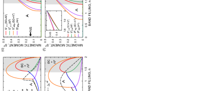
Figure 1: (Color online) Stable phases evolution vs. band filling. The superconducting gap parameter, magnetic moment and free energies as a function of band filling both for the HF and SGA, for $J=0.299$: a, b, c and $J=0.4545$: d, e, f. The results are for $\beta_{h}=0.0$. The shaded regions represent the stability regions of the respective phases according to the SGA calculations. In Figs. a and d we show only the free energies of stable phases. The arrows in a and d mark the transitions points between phases.

One should note that in the considered regime ($U<3J$) we have a model with intraatomic interorbital attractions leading to spin-triplet pairs. As the main attractive force is of intraatomic nature, we focus here on the local (s-wave) type of pairing only. In other words, as we discuss the situation with no or small hybridization, the intersite part of the pairing can be disregarded.

The calculations have been carried out for $U^{\prime}=U-2J$, $U=2.2J$, $k_{B}T/W=10^{-4}$. This leaves us still with three independent microscopic parameters in our model: $n_{G}$, $J$, and $\beta_{h}$. All the energies have been normalized to the bare band-width $W=8|t|$ (as we consider the square lattice with nearest neighbor hopping). For comparison, we also show the results calculated by means of the combined HF-BCS$\equiv$HF approximation. This method is described in detail in our previous paper for the same model as considered here. We can also reproduce the HF results by using the Gutzwiller method described in this work and setting $\lambda_{I,I^{\prime}}=\delta_{I,I^{\prime}}$.

In Fig. 1 we display the free energy, superconducting gaps, and magnetic moments for the two values $J=0.299$ and $J=0.4545$. As one can see from the free-energy plots (Figs. 1a and 1d), below some certain value of band filling, the pure superconducting phase of type A is stable for the SGA method. The increase of the number of electrons in the system, enhances the gap in this region (Figs. 1b and 1e). Above the critical band filling $n_{c}$, the staggered moment structure is created and a division into two gap parameters ($\Delta_{+}$ and $\Delta_{-}$) appears, as can be seen in Figs. 1b, 1e, 1c, and 1f. In this regime the SC+AF phase becomes stable.

When approaching half filling, both gaps gradually approach zero and for $n=2$ we are left with a pure AF phase, which is of Slater insulating type evolving towards the Mott-Hubbard insulating state with the increasing U. As the staggered magnetic moment is rising (with the increase of $n_{G}$), the renormalization factor is approaching unity (cf. Insets to Fig. 1a and 1d). This is a consequence of the fact that for large values of $S^{z}_{G}$, the configurations with two electrons of opposite spin, on the same orbital, are ruled out.

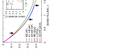
Figure 2: (Color online) The superconducting gaps (a) and the free energies (b) as a function of band filling for $J=0.4545$ and $\beta_{h}=0.1$. The shaded regions represent stability of respective phases according to the SGA calculations. The vertical arrows mark the phase borders.

Comparing Figs. 1a, 1b, 1c with Figs. 1d, 1e, 1f one sees that by increasing $J$ we make the value of $n_{c}$ smaller. However, the decrease in $n_{c}$ is not as significant in SGA as it is in the HF case. In general the results presented Figs. 1b, 1c, 1e, 1f look similar from the qualitative point of view for both methods. For SGA, the onset of antiferromagnetically ordered phase appears closer to half filling than for the HF method. Another difference between HF and SGA is that for the former the staggered moment in the SC+AF phase is increased by the appearance of SC for the whole range of band fillings, whereas in SGA calculations the staggered moment is slightly stronger in the AF phase than in the SC+AF phase for a small region close to the half-filled situation (inset of Fig. 1f).

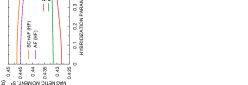
Figure 3: (Color online) The superconducting gaps and magnetic moment as a function of the hybridization strength, $\beta_{h}$, for $n=1.9$, $J=0.4545$, for the case of SC+AF and AF phases.

Significant differences between HF and SGA can be seen in Figs. 1c and 1f. While changing the band filling from 0 to 2, in the case of SGA calculations we move consecutively through the regions of stability of NS (for $J=0.299$), A, SC+AF phases, and for $n=2$ we have pure antiferromagnetism. The situation is different in the HF approximation, where in between the regions

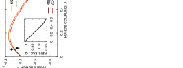
Figure 4: (Color online) The superconducting gaps in the SC+AF phase (a) and free energies of stable phases (b) as a function of Hund’s coupling for $n=1.9$ and $\beta_{h}=0.1$. The shaded region represent the stability of NS phase according to the SGA results.

of stability of A and SC+AF phase, we have also the stable A1+FM phase. It should be also noted that the free energy calculated in SGA is lower than the one for the HF situation, as one should expect, since the correlations are accounted more accurately in the former method. It is also very interesting that having the system with $U<3J$, no pure ferromagnetism appears in this canonical model of itinerant magnetism.

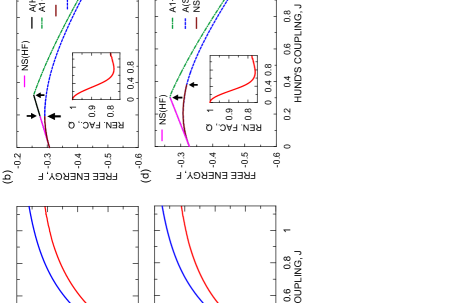
Figure 5: (Color online) The superconducting gaps in the A phase as a function of the Hund’s coupling for $n=1.0$ (a-for $\beta_{h}=0.0$ and c-for $\beta_{h}=0.1$) and free energies of stable phases corresponding to SGA and HF approximations (b-for $\beta_{h}=0.0$ and d-for $\beta_{h}=0.1$). The shaded regions represent the stability of the NS phase according to the SGA. The vertical arrows mark the border points between respective phases. Insets: Bandwidth renormalization factor for $\beta_{h}=0$ (upper) and $\beta_{h}=0.1$ (lower).

In Fig. 2, we present the results for the case with nonzero hybridization parameter, $\beta_{h}=0.1$. In this case there are no superconducting solutions below some certain value of the band filling (cf. Fig. 2a) and an extended region of NS stability occurs. The influence of the hybridization on the antiferromagnetically ordered phases is weak, as can be seen more clearly in Fig. 3. The changes in the superconducting gap and the magnetic moment triggered by the hybridization, are quite small even for larger values of $\beta_{h}$.

Next, we discuss the $J$ dependence of the superconducting gap, the free energy and the magnetic moment for selected values of band filling. As in the case of $n$-dependences the gap parameters and the magnetic moments in both SGA and HF approximation are qualitatively similar. In Fig. 4 we can see that for $n=1.9$ even the free-energy plots and regions of stability of certain phases are comparable for both calculation schemes used. For the quarter-filled case (cf. Fig. 5) the A1+FM phase is stable above some value of $J$, according to the HF results. However, this is not the case in the SGA approximation, where the A phase has lower free energy even than the saturated ferromagnetic phase coexisting with superconductivity. Comparing Figs. 5b and 5d (as well as 1d and 2b) one sees that the region of stability of the A phase narrows down in favor of the NS phase, due to the influence of hybridization.

It is important to check whether the itinerant magnetic phases are stable in the regime $U^{\prime}>J$ ($U>3J$), i.e., when the superconductivity is absent in the HF approximation. For this purpose, in Fig. 6 we provide the band-filling dependence of the free energy corresponding to stable phases for $U=4J$. Indeed, the paramagnetic and the magnetically ordered phases are stable for both methods of calculations. Therefore, for $U>3J$ we recover the magnetic phase diagram for this model, which was considered originally only in the context of magnetism. The free energy of the saturated ferromagnetic phase calculated by the SGA is very close to the one obtained by the HF approach. This is again caused by the circumstance that in the saturated state all of the spins are parallel and the double occupancies on the same orbital are absent. In this situation, the intra-orbital Coulomb interaction is automatically switched off. It would be interesting to determine the stability of the coexistent phases in this regime ($U^{\prime}>J$). Work along this line is in progress.

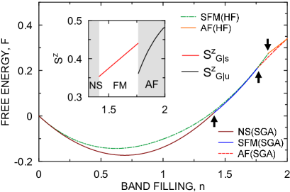
Figure 6: (Color online) The free energies of the stable phases for SGA and HF methods for $J=0.4$ and $U=1.6$. The shaded regions in the inset mark the stability of certain phases according to the SGA approach. Note the appearance of ferromagnetic phase for $U=4J$ (i.e., for $U>3J$) in the filling range $1.45\div 1.75$, sandwiched in between paramagnetic and antiferromagnetic phases.

Table 4: Exemplary values of the order parameters, the chemical potential, the free energy, and the band renormalization factors corresponding to the considered phases, for two different sets of values of the microscopic parameters $n$ and $J$. The underlined values correspond the stable phases. The numerical accuracy is on the level of the last digit specified.

		$n=1.0$	$n=1.9$
parameter	phase	$J=0.299$	$J=0.299$
$\Delta$	A	0.0450027	0.1701940
$\Delta$	A1+FM	0.0426749	0.1307664
$\Delta_{+}$	SC+AF	-	0.1638992
$\Delta_{-}$	SC+AF	-	0.0161868
$S^{z}_{u}$	A1+FM	0.000317	0.1092674
$S^{z}_{s}$	SC+AF	-	0.3902738
$S^{z}_{s}$	AF	-	0.3885899
$\mu$	A	-0.1382377	0.16078601
$\mu$	NS	-0.1377649	0.1875964
$\mu$	A1+FM	-0.1379700	0.18222514
$\mu$	SC+AF	-	-0.0421144
$\mu$	AF	-	-0.0893963
$F$	A	-0.3106091	-0.3118381
$F$	NS	-0.3105145	-0.2992516
$F$	A1+FM	-0.3105586	-0.3020254
$F$	SC+AF	-	-0.3576542
$F$	AF	-	-0.3509731
$Q_{\uparrow}$	A1+FM	0.8845776	0.6751619
$Q_{\downarrow}$	A1+FM	0.8839251	0.6282452
$Q$	A	0.8845136	0.6736373
$Q$	NS	0.8840340	0.6421089
$Q$	SC+AF	-	0.9211224
$Q$	AF	-	0.9293567

4 Conclusions and outlook

4.1 Conclusions

The principal purpose of this paper was to formulate a many-particle method which allows to investigate the spin-triplet real-space pairing in correlated system with an orbital degeneracy. To this end, we have carried out a detailed analysis using the statistically-consistent Gutzwiller approximation (SGA) for the two-band degenerate Hubbard model with the spin-triplet superconductivity and itinerant magnetism included, both treated on equal footing. The results were compared with those coming from the Hartree-Fock approximation amended with the Bardeen-Cooper-Schrieffer (BCS) approach. The obtained Hund’s coupling and band filling dependences of the magnetic moment and the superconducting gap parameters are often similar from the qualitative point of view with those evaluated by means of the HF approximation. However, the stability regions of the considered phases are significantly different for the two applied methods. In SGA, the stable coexisting superconducting-ferromagnetic phase is absent while it appears in the HF approximation in a certain range of $J$ and $n$ values. Furthermore, the coexistence of the paired state with antiferromagnetism appears much closer to the half-filled situation in SGA than in HF approximation. For $n=2$ the superconductivity disappears and only the pure antiferromagnetism survives; this state can be termed a correlated Slater-insulator state, which evolves gradually into the Mott-Hubbard insulating state with increasing $U>1$ and $S^{z}_{G|s}\rightarrow 1/2$.

The influence of hybridization for both approximations is similar. With an increase of the $\beta_{h}$ parameter, the region of stability of the superconducting type-A phase narrows down in favor of the NS state. On the other hand, the antiferromagnetic phase is not affected in any significant manner by an increase of $\beta_{h}$.

The band renormalization factors approach unity as the interaction constants $J$, $U$ and $U^{\prime}$ tend to zero, what represents an additional test of our numerical results correctness. Generally, in the low-coupling limit our present results reduce to those obtained in HF approximation analysed by us in [22], as it should be.

It is important to emphasize that for both approaches the phase diagrams have been obtained for $U<3J$, i.e. for relatively low value of the Hubbard interaction U, or equivalently, for a relatively high value of the Hund’s rule exchange integral. A complete analysis of the present model would require studying the stability of the spin-triplet superconductivity and its coexistence with magnetic ordering in the complementary regime $U>3J$, where the magnetism is favored against superconductivity. This regime has been the subject in a number of earlier papers [24, 45, 46], as then both the intraorbital, as well as the interorbital interaction is repulsive, and lead in a natural manner to magnetic ordering.

4.2 Outlook: Extension and application to real systems

In connection with the remarks provided above, we would like to characterize briefly the possibility of extending the present model (1) to the uranium systems in which superconductivity and ferromagnetism coexist in an unambiguous manner [36]. First of all, the magnetic moment in those systems, particularly in UGe₂ and URhGe, is quite large, with an associated molecular field in the megagauss range, which most probably rules out any spin-singlet character of pairing (note that the Curie temperature ($T_{C}$) to the superconducting transition temperature ($T_{S}$) ratio reaches in the uranium compounds the value $T_{C}/T_{S}\sim 10^{2}$). In spite of those circumstances, our solution does not provide any extended regime (for the studied parameter range) for the ferromagnetism-spin-triplet superconductivity coexistence. Instead, in a wide range of band fillings, the coexisting SC+AF phase is stable (cf. Fig. 1c and 1f), as well as the pure spin-triplet superconducting phase of type A (the equal-spin-paired phase). The pure A phase seems to be realized in Sr₂RuO₄, though then a detailed three-orbital structure of the order parameter seems to be relevant [40]. A direct application of our SGA scheme to a realistic three-band system is more involved, as the number of parameters to minimize would lead to a computing time-consuming procedure, but still possible to tackle.

The extension of the present model to the uranium system such as UGe₂ would require considering orbitally degenerate and correlated $5f^{2}-5f^{3}$ quasi-atomic states due to U and hybridized with the uncorrelated conduction band states. This means that we must have minimally a three-orbital system with two partially occupied $5f$ quasi-atomic states (so the Hund’s rule becomes operative) and at least one extra conduction band. Such situation may lead to a partial Mott-localization phenomenon, i.e., to a spontaneous decomposition of $5f^{n}$ ($n>1$) configuration of electrons into the localized and the itinerant parts [41]. In such a situation, it is possible that the localized electrons are the source of ferromagnetism, whereas the itinerant particles are paired [9]. This is not the type of coexistent phase we have in mind here, since in the model considered by us all the system electrons are indistinguishable in the quantum-mechanical sense.

These considerations lead to the conclusion that one would require minimally a periodic Anderson model with degenerate $5f^{n}$ states, to mimic the uranium-based ferromagnetic superconductors. This variant of the multiple-band model is also very useful in the discussion of heavy-fermion compounds. Moreover, in the systems represented by this model, the coexistence of antiferromagnetism and superconductivity has been shown to appear in both experiment [48] and theory [49]. More specifically for the systems UPt₃ and UNi₂Al₃ the coexistence of the spin-triplet pairing and the antiferromagnetism has already been suggested to appear [50, 51], although not elaborated in any detail. One specific feature should be mentioned. Namely, in the situation when we have antiferromagnetic superconductor, then there is also a strong theoretical indication that there is a spin-triplet component even for the pure spin-singlet mechanism of pairing [27, 49]. The spin-triplet important admixture results simply from a decomposition of the system into two sublattices with staggered magnetic moment. These and related features must be taken into quantitative analysis before any realistic consideration of concrete systems is carried out.

In connection with the whole discussion, it is intriguing to ask if a symmetric model system of the type exemplified by Hamiltonian (1) could be experimentally realized in the optical lattice. Some model systems (e.g., the Hubbard model system) have been experimentally achieved in this manner [42].

In relation to the spin-triplet real-space pairing induced by the Hund’s rule, one should also mention the spin fluctuations (SF) as a possible mechanism of spin-triplet pairing in both magnetic [42] and liquid ³He systems [43]. Within the present approach the spin fluctuations should be treated as quantum fluctuations around the present self-consistently renormalized mean field state [44]. The real-space and the spin-fluctuation contributions may become of comparable magnitude in the close vicinity of the quantum critical point, where the ferro- or antiferro- states disappear under e.g. pressure. This is, however, a completely separate topic of studies.

5 Acknowledgements

Disscusions with Jakub Jędrak and Jan Kaczmarczyk are gratefully acknowledged. M.Z. has been partly supported by the EU Human Capital Operation Program, Polish Project No. POKL.04.0101-00-434/08-00. J.S. acknowledges the financial support from the Foundation for Polish Science (FNP) within project TEAM. The grant MAESTRO from the National Science Center (NCN) was helpful for the PL-DE cooperation within the present project on a unified approach to magnetism and superconductivity in correlated fermion systems.

References

References

- [1] Y. Maeno, H. Hashimoto, K. Yoshida, S. Nishizaki, T. Fujita, J, G. Bednorz and F. Lichtenberg, Nature 372, 532 (1994).
- [2] Y. Maeno, Physica B 281-282, 865 (2000)
- [3] S. S. Saxena, P. Agarwal, K. Ahilan, F. M. Grosche, R. K. W. Haselwimmer, M. J. Steiner, E. Pugh, I. R. Walker, S. R. Julian, P. Monthoux, G. G. Lonzarich, A. Huxley, I. Sheikin, D. Braithwaite and J. Flouquet, Nature 406, 587 (2000).
- [4] A. Huxley, I. Sheikin, E. Ressouche, N. Kemovanois, D. Braithwaite, R. Calemczuk, J. Flouquet, Phys. Rev. B 63, 144519 (2001).
- [5] N. Tateiwa, T. C. Kobayashi, K. Hanazono, K. Amaya, Y. Haga, R. Settai and Y. Onuki, J. Phys.: Condens. Matter 13, 117 (2001).
- [6] T. C. Kobayashi, S. Fukushima, H. Hidoka, H. Kotegawa, T. Akazawa, E. Yamamoto, Y. Haga, R. Settai, and Y. Onuki, Physica B 378-380, 355 (2006).
- [7] N. T. Huy, A. Gasparini, D. E. de Nijs, Y. Huang, J. C. P. Klaasse, T. Gortenmulder, A. de Visser, A. Hamann, T. Görlach, and H. v. Löhneysen, Phys. Rev. Lett. 99, 067006 (2007).
- [8] E. Slooten, T. Naka, A. Gasparini, Y. K. Huang, and A. de Visser, Phys. Rev. Lett. 103, 097003 (2009).
- [9] For review see: A. de Visser in Encyclopedia of Materials Science: Science and Technology (Elsevier, 2010), pp. 1-6.
- [10] C. Geibel, S. Thies, D. Kaczorowski, A. Mehner, A. Grauel, B. Seidel, U. Ahlheim, R. Helfrich, K. Petersen, C. D. Bredl, and F. Staglich, Z. Phys. B 83, 305 (1991).
- [11] A. Schröder, J. G. Lussier, B. D. Gaulin, J. D. Garrett, W. J. L. Buyers, L. Rebelski, and S. M. Shapiro, Phys. Rev. Lett. 72, 1 (1994).
- [12] K. Ishida, D. Ozaki, T. Kamatsuka, H. Tou, M. Kyogaku, Y. Kitaoka, N. Tateiwa, N. K. Sato, N. Aso, C. Geibel, and F. Steglich, Phys. Rev. Lett. 89, 3 (2002).
- [13] G. Aeppli, D. Bishop, C. Broholm, E. Bucher, K. Siemensmeyer, M. Steiner, and N. Stüsser, Phys. Rev, Lett. 63, 6 (1989)
- [14] H. Tou, Y. Kitaoka, K. Asayama, N. Kimura, Y. Onuki, E. Yamamoto, and K. Maezawa, Phys. Rev. Lett. 77, 7 (1996)
- [15] K. Klejnberg and J. Spałek, J. Phys.: Condens. Matter 11, 6553 (1999).
- [16] K. Klejnberg and J. Spałek, Phys. Rev. B 61, 15542 (2000).
- [17] J. Spałek, Phys. Rev. B 63, 104513 (2001).
- [18] J. Spałek, P. Wróbel, and W. Wójcik, Physica C 387, 1 (2003).
- [19] Previous brief and qualitative considerations about the ferromagnetism and spin-triplet pairing coexistence see: S-Q. Shen, Phys. Rev. 57, 6474 (1998).
- [20] M. Zegrodnik and J. Spałek, Acta Phys. Pol. A 121 1051 (2011).
- [21] M. Zegrodnik and J. Spałek, Acta Phys. Pol. A 121 801 (2011).
- [22] M. Zegrodnik and J. Spałek, Phys. Rev. B 86 014505 (2012).
- [23] J. Bünemann and W. Weber, Phys. Rev. B 55 4011 (1997).
- [24] J. Bünemann, W. Weber and F. Gebhard, Phys. Rev. B 57 6896 (1998).
- [25] Jörg Bünemann, Florian Gebhard, Torsten Ohm, Stefan Weiser, and Werner Weber in Frontiers in Magnetic Materials (Springer, Berlin 2005).
- [26] J. Jędrak and J. Spałek, Phys. Rev. B 81 073108 (2010).
- [27] J. Kaczmarczyk and J. Spałek, Phys. Rev. B 84 125140 (2011).
- [28] O. Howczak and J. Spałek, J. Phys.: Condens. Matter 24 205602 (2012).
- [29] J. Jędrak, J. Kaczmarczyk and J. Spałek, arXiv:1008:0021v2 [cond-mat.str-el] 18 May 2011.
- [30] K. Sano and Y. Ōno, J. Phys. Soc. Jpn., 72, 1847 (2003).
- [31] J. E. Han, Phys. Rev. B 70, 054513 (2004).
- [32] J. Hotta and K. Ueda, Phys. Rev. Lett. 92, 107007 (2004)
- [33] X. Dai, Z. Fang, Y. Zhou, and F-C. Zhang, Phys. Rev. Lett 101, 057008 (2008).
- [34] P. A. Lee and X-G. Wen, Phys. Rev. B 78, 144517 (2008).
- [35] Y. Imai, K. Wakabayashi, M. Sigrist, Phys. Rev. B 85, 174532 (2012).
-
[36]
J. Jędrak, Ph.D. Thesis, Jagiellonian University (Kraków, 2011);
th-www.if.uj.edu.pl/ztms/download/phdTheses/
Jakub_Jedrak_doktorat.pdf - [37] J. Bünemann, F. Gebhard, T. Schickling, and W.Weber, phys. stat. sol. (b) 248, 203 (2010).
- [38] J. Bünemann, F. Gebhard, and R. Thul, Phys. Rev. B 67, 075103 (2003).
- [39] The first observation of weak ferromagnetism-superconductivity coexistence for the same electrons was reported in: A. Kołodziejczyk, B. V. B. Sarkissian, and B. R. Coles, J. Phys. F: Met. Phys. 10, L333 (1980). However, as the phases coexist only in a narrow range of temperatures the pairing is most probably of the spin-singlet nature, cf. B. Wiendlocha, J. Toboła, S. Kaprzyk, and A. Kołodziejczyk, Phys. Rev B 83, 094408 (2011).
-
[40]
J. F. Annet, B. L. Györffy, and K. I. Wysokiński, New J. Phys. 11,
055063 (2009);
K. I. Wysokiński, J. F. Annet, and B. L. Györffy, Phys. Rev. Lett. 108, 1077004 (2012). - [41] G. Zwicknagl, J. Phys. Soc. Japan, 75 Suppl., 226 (2006), and references therein.
- [42] For review see: I. Bloch, J. Dalibard, and W. Zwerger, Rev. Mod. Phys. 80, 885 (2008)
-
[43]
D. Fay and J. Appel, Phys. Rev. B 22, 3173 (1980);
A. Layzer and D. Fay, Inter. J. Magnetism, 1, 135 (1971). - [44] P. W. Anderson and W. F. Brinkman in The Physics of Liquid and Solid Helium, edited by K. H. Bennemann and J. B. Ketterson (J. Wiley, New York, 1977), p. 177ff
- [45] J. Kunes̆, I. Leonov, M. Kollar, K. Byczuk, V. I. Anisimov, and D. Vollhardt, Eur. Phys. J. Special Topics, 180, 5 (2010).
- [46] X. Y. Deng, L. Wang, X. Dai, and Z. Fang, Phys. Rev. B 79, 075114 (2009).
-
[47]
A. Klejnberg, Ph.D. Thesis, Jagiellonian University (Kraków, 2007);
th-www.if.uj.edu.pl/ztms/download/phdTheses/
Andrzej_Klejnberg_doktorat.pdf (in Polish). - [48] For recent review see: G. Knebel, J. Buhot, D. Aoki, G. Laperot, S. Raymond, E. Ressouche, and J. Flouquet, J. Phys. Soc. Jpn. 80, SA001(2011).
- [49] O. Howczak, J. Kaczmarczyk, and J. Spałek, arXiv: 1209.0621 and Phys. Stat. Solidi (b), in press.
- [50] D. van der Marel and G. A. Sawatzky, Sol. St. Commun. 55, 937 (1985).
-
[51]
P. W. Anderson, Phys. Rev. B 30, 1549 (1984);
M. R. Norman, Phys. Rev. Lett. 72, 2077 (1994).