Hybrid functionals for solids with an optimized Hartree-Fock mixing parameter

Abstract

(Screened) hybrid functionals are being used more and more for solid-state calculations. Usually the fraction $\alpha$ of Hartree-Fock exchange is kept fixed during the calculation, however there is no single (universal) value for $\alpha$ which systematically leads to satisfying accuracy. Instead, one could use a property of the system under consideration to determine $\alpha$ and in this way the functional would be more flexible and potentially more accurate. Recently, it was proposed to use the static dielectric constant $\varepsilon$ for the calculation of $\alpha$ [Shimazaki and Asai, Chem. Phys. Lett. 466, 91 (2008) and Marques et al., Phys. Rev. B 83, 035119 (2011)]. We explore this idea further and propose a scheme where the connection between $\varepsilon$ and $\alpha$ is optimized based on experimental band gaps. $\varepsilon$, and thus $\alpha$, is recalculated at each iteration of the self-consistent procedure. We present results for the band gap and lattice constant of various semiconductors and insulators with this procedure. In addition, we show that this approach can also be combined with a non-self-consistent hybrid approximation to speed up the calculations considerably, while retaining an excellent accuracy in most cases.

I Introduction

Hybrid functionals,Becke (1993a, b) and in particular the screened versions,Bylander and Kleinman (1990); Heyd et al. (2003); Tran and Blaha (2011) provide, in combination with a generalization (Ref. Seidl et al., 1996) of the Kohn-Sham equations,Kohn and Sham (1965) an efficient way to deal with the well-known band gap problemPerdew (1985); Kümmel and Kronik (2008) in density functional theory (DFT). Hohenberg and Kohn (1964) In hybrid functionals, (semi)local [i.e., local density (LDA) or generalized gradient approximation (GGA)] and Hartree-Fock (HF) exchange are mixed, and since the trends of pure semilocal and pure HF methods is to underestimate and overestimate band gaps, respectively, the mixing of both usually leads to more accurate band gaps. The use of hybrid functionals has been justified by (more or less) formal arguments (Refs. Becke, 1993a and Perdew et al., 1996a).

One well-established screened hybrid functional for solids is the one proposed by Heyd, Scuseria, and ErnzerhofHeyd et al. (2003) (HSE), which is based on the GGA functional of Perdew, Burke, and ErnzerhofPerdew et al. (1996b) (PBE):

$$E_{\text{xc}}=\alpha E_{\text{x}}^{\text{SR,HF}}+(1-\alpha)E_{\text{x}}^{\text{SR,PBE}}+E_{\text{x}}^{\text{LR,PBE}}+E_{\text{c}}^{\text{PBE}},$$ (1)

where $\alpha$ ($\in[0,1]$) is the mixing parameter for the short-range exchange (in screened hybrid functionals the long-range exchange is pure semilocal). The indices “x” and “c” denote the exchange and correlation energy contributions. The HSE functional is usually used with $\alpha=0.25$. Another parameter in Eq. (1) is the screening parameter $\lambda$ in the error function ($\lambda=0.11$ bohr^-1 in the version HSE06Krukau et al. (2006)), which determines the separation between short-range and long-range exchange. A larger amount $\alpha$ of HF exchange increases the band gap, while a larger value for $\lambda$ (i.e., more screening) decreases it. Actually, this means that depending on the choice of these two parameters more or less any desired result between PBE and HF can be obtained. Furthermore, it also means that a reasonable way to fix the parameters is very important. In the HSE06 functional, the first of these parameters ($\alpha$) was chosen on the basis of theoretical considerations,Perdew et al. (1996a) whereas the second one ($\lambda$) was fitted to experimental results.Heyd et al. (2003) It has been shown that by fitting both parameters further improvement can be achieved.Moussa et al. (2012)

At this point, it is worth recalling that already in 1990 Bylander and Kleinman Bylander and Kleinman (1990) proposed an LDA-based functional containing screened HF exchange (sX-LDA):

$$E_{\text{xc}}=E_{\text{x}}^{\text{SR,HF}}+E_{\text{x}}^{\text{LR,LDA}}+E_{\text{c}}^{\text{LDA}},$$ (2)

which can be regarded as a hybrid functional with $\alpha=1$. In the sX-LDA functional, the long-range and short-range exchange are split using the exponential function (Yukawa potential).

Up to now, the majority of calculations with hybrid functionals (full-range, short-range, or long-range) have been done with fixed values for $\alpha$ and $\lambda$. However, allowing $\alpha$ or $\lambda$ to depend on a property of the system is a way to make the functional more flexible and thus potentially more accurate. A brief summary of such schemes is mentioned below. The sX-LDA functional is usually used with a screening parameter $\lambda$ which is calculated using the average of the valence electron density (see, e.g., Ref. Clark and Robertson, 2010 for recent calculations). In Ref. Jaramillo et al., 2003, it was proposed to make $\alpha$ position-dependent by using the electron density $\rho$, its derivative $\nabla\rho$, and the kinetic-energy density, while in Ref. Krukau et al., 2008, the use of a position-dependent $\lambda$ which depends on $\rho$ and $\nabla\rho$ has been proposed. Shimazaki and Asai Shimazaki and Asai (2008, 2009, 2010) proposed several functionals in which either both $\alpha$ and $\lambda$ or only $\alpha$ are determined using the static dielectric constant $\varepsilon_{s}$. In the method presented in Ref. Stein et al., 2010 by Stein et al., the screening parameter is tuned such that the Koopmans’ theorem (which requires the use of orbital eigenvalues and total energies) is obeyed as closely as possible. Marques et al. Marques et al. (2011) considered two ways for the calculation of $\alpha$: either with the static dielectric constant $\varepsilon_{s}$ or with the average of $\left|\nabla\rho\right|/\rho$ in the unit cellMarques et al. (2011) (as done originally in a similar context for the modified Becke-Johnson exchange potentialTran and Blaha (2009)). We also mention that interesting discussions about the link between screened hybrid functionals and quasiparticle theories can be found in Refs. Marques et al., 2011 and Moussa et al., 2012.

In the present work, we further explore the use of the dielectric constant for the calculation of the fraction of HF exchange in the screened hybrid functional YS-PBE0,Tran and Blaha (2011) which is based on the Yukawa operator. We will show the results obtained with this scheme for the band gap and lattice constant of solids. Our work is organized as follows. In Sec. II the computational details are given, while the description of our method and the results are presented in Sec. III. Finally, the summary of our work will be given in Sec. IV.

II Computational Details

All calculations were performed with the WIEN2k software,Blaha et al. (2001) which is based on the full potential (linearized) augmented plane wave and local orbitals methodSingh and Nordström (2006) for quantum calculations on periodic systems. Recently, unscreened and screened hybrid functionals were implemented into WIEN2k.Tran and Blaha (2011) In screened hybrid functionals, the screening of the Coulomb operator is done by using the exponential function, and it was shown (Ref. Tran and Blaha, 2011) that by choosing carefully the screening parameter $\lambda$, the results are very close to the results from the error function-based screened hybrid functionals (e.g., HSE06). More specifically, the screening parameter used in the exponential function should be about $1.5$ times larger than the one used for the error function (see Refs. Shimazaki and Asai, 2008, 2009, 2010; Tran and Blaha, 2011 for details). The results presented in the present work were obtained with the YS-PBE0 functional which is based on the PBE functionalPerdew et al. (1996b) and was used in our previous works.Botana et al. (2012); Tran et al. (2012) The YS-PBE0 calculations were done with a fixed screening parameter of $\lambda=0.165$ bohr^-1, which gives results close to the results obtained with the HSE06 functional.Krukau et al. (2006) Spin-orbit coupling has not been considered explicitly in hybrid functional calculations, but its influence on the band gap is considered to be the same as for the PBE functional and the gaps have been corrected accordingly.

The imaginary part of the dielectric function $\varepsilon$ was calculated using Fermi’s golden rule and the independent particle approximation. The Kramers-Kronig transformation was used to obtain the real part of $\varepsilon$. Details of this approach can be found in Ref. Ambrosch-Draxl and Sofo, 2006. This gives the $G=G^{\prime}=0$ element of the dielectric matrix from which the static macroscopic dielectric constant (which is a tensor since solids are anisotropic) can be obtained by taking the limit $\omega\rightarrow 0$ and $\mathbf{q}\rightarrow 0$ of the real part. For solids whose symmetry leads to vanishing off-diagonal elements of this tensor we take the geometric mean of the diagonal elements of this tensor and from now on we will refer to it simply as the dielectric constant and use the symbol $\varepsilon^{*}$. Systems with non-vanishing off-diagonal elements were not considered in the present work. All parameters of the calculations, such as basis-set size or Brillouin zone sampling were tested for convergence. Except for the calculations of the lattice constants, the experimental structures have been used.

III Results and Discussion

III.1 Band gap

Table 1: Fundamental band gaps (in eV) of 24 solids categorized into four different groups: ionic compounds, $sp$-semiconductors, transition-metal oxides (labeled as “TmO”), and other transition-metal compounds (labeled as “TmX”). The Strukturbericht symbols are indicated in parenthesis. The three columns “YS-PBE0” show the results obtained with the hybrid functional YS-PBE0 with $\alpha=0.25$ (Sec. III.1), $\alpha_{\text{opt}}$ (Sec. III.1), and $\alpha_{\text{opt}}$ with the non self-consistent diagonal-HF approximation (Sec. III.3). The experimental band gaps (see Ref. Koller et al., 2012 for the references) are shown for comparison. In addition, $\alpha_{\text{opt}}$ (obtained from the fitting procedure), and the static dielectric functions obtained from YS-PBE0 ($\alpha_{\text{opt}}$), PBE, and experiment are also shown.

Solid	Type	YS-PBE0 ($\alpha=0.25$)	YS-PBE0 ($\alpha_{\text{opt}}$)	YS-PBE0-diag ($\alpha_{\text{opt}}$)	exp.	$\alpha_{\text{opt}}$	$\varepsilon^{*}_{\alpha_{\text{opt}}}$	$\varepsilon^{*}_{\text{PBE}}$	$\varepsilon_{\text{exp}}$
LiF (B1)	ionic	11.4	14.5	15.1	14.2	0.58	1.5	2.1	1.9
NaF (B1)	ionic	8.4	11.9	12.5	11.7	0.63	1.3	1.8	1.7
KF (B1)	ionic	8.1	11.0	11.8	10.9	0.59	1.4	2.0	1.8
LiCl (B1)	ionic	7.8	9.0	8.9	9.4	0.45	2.1	3.3	2.7
NaCl (B1)	ionic	6.5	7.9	7.9	8.6	0.50	1.8	2.7	2.3
KCl (B1)	ionic	6.5	8.0	8.1	8.5	0.52	1.7	2.6	2.2
CaO (B1)	ionic	5.3	6.5	7.2	7.0	0.43	2.3	3.9	3.3
C (A4)	$sp$	5.4	5.5	5.5	5.48	0.30	4.0	5.8	5.7
Si (A4)	$sp$	1.16	1.08	1.07	1.17	0.22	8.2	12.9	11.9
Ge (A4)	$sp$	0.77	0.61	0.53	0.74	0.20	11.4	20.8	15.9
CdS (B3)	$sp$	2.12	2.42	2.44	2.42	0.32	3.7	6.3	5.3
GaN (B3)	$sp$	2.8	3.2	3.2	3.2	0.32	3.6	6.0	5.3
BN (B3)	$sp$	5.8	6.4	6.3	6.25	0.35	3.2	4.6	4.5
SiC (B3)	$sp$	2.25	2.40	2.38	2.4	0.29	4.6	7.0	6.5
AlP (B3)	$sp$	2.29	2.35	2.33	2.45	0.27	5.4	8.5	7.5
InP (B3)	$sp$	1.42	1.39	1.37	1.42	0.24	6.7	10.9	9.6
Cu2O (C3)	TmO	1.89	2.25	2.51	2.17	0.31	3.8	9.3	6.5
TiO2 (C4)	TmO	3.3	3.7	5.5	3.3	0.31	4.0	7.9	6.3
ZnO (B4)	TmO	2.5	3.7	4.5	3.44	0.42	2.4	4.9	3.7
SrTiO3 (E21)	TmO	3.2	3.8	5.6	3.25	0.34	3.4	6.3	5.2
MnO (B1)	TmO	2.9	3.8	4.6	3.9	0.37	2.8	7.7	5.0
ScN (B1)	TmX	0.84	0.84	—	0.9	0.25	5.9	12.1	7.2
MoS2 (C7)	TmX	1.44	1.33	1.32	1.29	0.22	9.0	13.9
ZnS (B3)	TmX	3.3	3.7	3.7	3.91	0.32	3.7	6.2	5.1

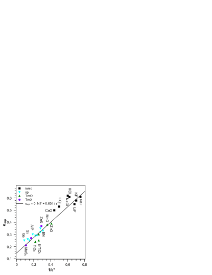
Figure 1: (Color online) The fraction of HF exchange required to reproduce the experimental band gap ($\alpha_{\text{exp}}$) versus the inverse of the dielectric constant ($1/\varepsilon^{*}$) which is obtained from a YS-PBE0 calculation using the corresponding $\alpha_{\text{exp}}$. The straight line [$\alpha_{\text{opt}}=\alpha_{\text{opt}}(\varepsilon^{*})$] is a fit corresponding to the least square error of the gap and not of $\alpha$.

Figure 2: (Color online) Difference between calculated (full symbols: YS-PBE0 with $\alpha_{\text{opt}}$, open symbols: YS-PBE0 with $\alpha=0.25$) and experimental band gaps. The shape of the symbol indicates the type of solids.

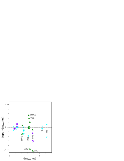
Figure 3: (Color online) Same as Fig. 2, but only for solids with band gaps smaller than 7 eV.

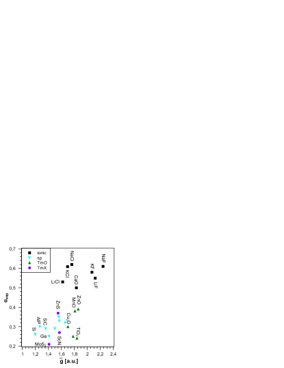
Figure 4: (Color online) The fraction of HF exchange required to reproduce the experimental band gap ($\alpha_{\text{exp}}$) versus $\overline{g}$ (see text for definition).

Hybrid functionals with fixed amount of exact exchange and screening length can be problematic if applied to different types of systems. For instance HSE is knownMatsushita et al. (2011) to work well for many small-gap semiconductors but strongly underestimates the gaps of highly ionic compounds such as NaCl. This means that in order to find an hybrid functional with broader applicability, it is important to include different types of solids in the fitting set. The solids that we considered for this study are listed in Table 1. They include highly ionic compounds with large band gaps, technologically important $sp$-semiconductors and more or less strongly correlated transition-metal compounds which can be split further into oxides (TmO) and non-oxides (TmX).

As already mentioned, the dielectric constant $\varepsilon^{*}$ will be used for the determination of the fraction $\alpha$ of HF exchange. Note that in the present work, the screening parameter $\lambda$ has been kept fixed at $\lambda=0.165$ bohr^-1 (Ref. Tran and Blaha, 2011) to make comparison with YS-PBE0 (and therefore HSE06) possible. As we can see from Fig. 1, choosing $\varepsilon^{*}$ seems to be a very good choice. Indeed, there is a nice linear correlation between $\alpha_{\text{exp}}$, which is the amount of HF exchange required to reproduce the experimental band gap and $1/\varepsilon^{*}$ which is obtained from a YS-PBE0 calculation using the corresponding $\alpha_{\text{exp}}$. We considered the linear relation $\alpha_{\text{opt}}=A+B/\varepsilon^{*}$ and a fit procedure minimizing the least-square error in the gaps leads to $A=0.147$ and $B=0.634$. Note, that our linear approximation does not go through the origin and the slope is not one, while in a previous work reported in Ref. Marques et al., 2011 a strict proportionality $\alpha=1/\varepsilon^{\text{PBE}}$ was used (in unscreened PBE0). The linear fit is shown in Fig. 1, where we can see that most data points are quite close to it. The exceptions are the ionic chlorides and the noble gases (not shown explicitly) whose $\alpha_{\text{exp}}$ are larger than the values $\alpha_{\text{opt}}$ obtained from the fit and rutile and strontium titanate, where $\alpha_{\text{exp}}$ is a bit smaller than the fitted $\alpha_{\text{opt}}$. Thus, it can be expected that the gaps of the chlorides will be underestimated, whereas the gaps of rutile and strontium titanate will be overestimated.

The resulting band gaps are listed in Table 1 and are compared with the values obtained with the standard fixed value $\alpha=0.25$. The band gaps are also plotted in Figs. 2 and 3 for a better comparison. It can be clearly seen that in nearly all cases, improved band gaps are obtained with $\alpha_{\text{opt}}$ compared to $\alpha=0.25$, and in some cases the improvement is quite impressive. In particular, the band gaps of the highly ionic compounds, which are knownMatsushita et al. (2011) to be underestimated by about 3 eV in HSE, are reproduced much more accurately with the $\varepsilon^{*}$-dependent $\alpha_{\text{opt}}$. As expected from Fig. 1, the use of $\alpha_{\text{opt}}$ leads to underestimations (which are much smaller than when HSE is used) for the chlorides and overestimations in the case of rutile and strontium titanate. For the other solids the performance can be considered as excellent. The deviation from experiment is within a range of $\pm 0.3$ eV which is quite good, since experimental errors and temperature effects need to be considered as well. The performance is even slightly better than that of the modified Becke-Johnson potential with the parameters suggested in Ref. Koller et al., 2012.

Since the static dielectric constant $\varepsilon^{*}$ is a central quantity in the described approach, it is important to compare the calculated values to the experimental results. Table 1 shows the values obtained from calculations (with PBE and YS-PBE0${}_{\alpha_{\text{opt}}}$) and experiment. We can see that YS-PBE0 with $\alpha_{\text{opt}}$ underestimates the experimental values by about 30%, contrary to PBE which slightly overestimates them. This is not surprising, since gaps are underestimated by PBE and lower gaps lead to higher dielectric constants. In our calculations, however, the dielectric function is calculated in the independent particle approximation and does not include electron-hole interactions, which would lead to an increase in the dielectric constants.Shishkin et al. (2007) An improved calculation for $\varepsilon^{*}$ would require a re-parameterization of $\alpha_{\text{opt}}$.

As a last remark in this section, we also mention that an alternative way to determine $\alpha$ would be to use

$$\overline{g}=\frac{1}{V_{\text{cell}}}\int\limits_{\text{cell}}\frac{\left|\nabla\rho(\mathbf{r})\right|}{\rho(\mathbf{r})}d^{3}r,$$ (3)

which is the average of $\left|\nabla\rho\right|/\rho$ in the unit cell and has been used successfully for the modified Becke-Johnson potential.Tran and Blaha (2009); Koller et al. (2011); Singh (2010); Koller et al. (2012) However, as Fig. 4 shows, the situation with $\overline{g}$ is quite different since there is no clear correlation between the values of $\alpha_{\text{exp}}$ and $\overline{g}$. Different classes of materials ($sp$-semiconductors, ionic chlorides or fluorides, transition metal compounds) would require drastically different parameterizations. The transition-metal oxides show only small variations in $\overline{g}$ but require quite different $\alpha_{\text{opt}}$, which is of course very problematic if any kind of relation $\alpha_{\text{opt}}=\alpha_{\text{opt}}(\overline{g})$ is desired. This is in quite strong contrast to the findings in Ref. Marques et al., 2011, where they found a good relation between $\alpha$ and $\overline{g}$. However, their set of solids was much more restricted in terms of transition-metal or highly ionic systems, and furthermore, their calculations were obtained with the pseudopotential plane wave method, whereas the calculations presented in the present work were obtained from an all-electron method, this difference leading certainely to different values of $\overline{g}$. Therefore, we considered only the parameterization in terms of the dielectric constant.

III.2 Lattice parameters

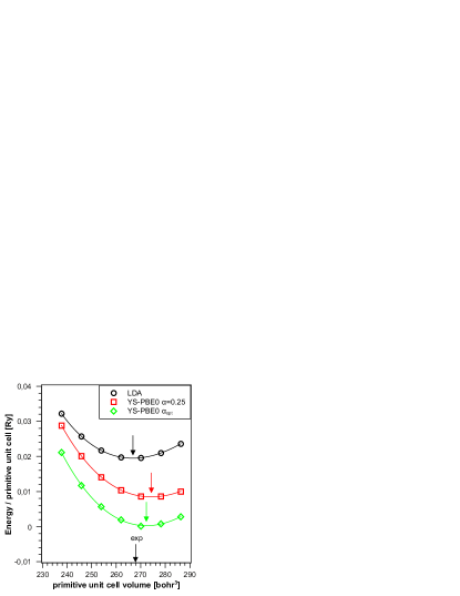
Figure 5: (Color online) Total energy of silicon as a function of atomic volume for 3 different functionals. The lines represent fits to the Birch-Murnaghan-EOS, the arrows indicate the corresponding minima.

Table 2: Comparison between theoretical and experimental lattice parameters (in Å) for several solids. All experimental values except ScN are corrected for zero-point anharmonic expansion.Haas et al. (2009) The values of $\alpha_{\text{opt}}$ and $d\alpha_{\text{opt}}/d\ln V$ at the experimental volume are also shown.

Solid	exp.	LDA	WC	HSE06	YS-PBE0	YS-PBE0	$\alpha_{\text{opt}}(V=V_{\text{exp}})$	$\frac{d\alpha_{\text{opt}}}{d\ln V}(V=V_{\text{exp}})$
					($\alpha=0.25$)	($\alpha_{\text{opt}}$)
C	3.54	3.54	3.56	3.55	3.55	3.55	0.306	$-0.025$
Si	5.42	5.41	5.44	5.44	5.46	5.44	0.224	$-0.015$
SiC	4.34	4.33	4.36	4.35	4.36	4.34	0.284	$-0.041$
BN	3.59	3.59	3.61	3.60	3.61	3.60	0.346	$-0.021$
GaN	4.52	4.46	4.50	4.49	4.52	4.50	0.323	$-0.098$
ScN	4.50	4.43	4.47		4.51	4.52	0.254	0.042
CaO	4.79	4.72	4.78		4.82	4.86	0.427	0.077
LiCl	5.07	4.97	5.07	5.12	5.15	5.55	0.447	0.15
NaCl	5.60	5.48	5.62	5.64	5.69	6.30	0.498	0.13

Another important test for functionals is the total energy, in particular how accurate equilibrium structural parameters or atomization energies can be described. Note, that $\alpha_{\text{opt}}$ will change as function of the lattice parameter and this could have important consequences on the equilibrium geometry. Therefore, we calculated the equilibrium lattice parameters for a few selected solids by calculating the total energies for different lattice parameters and fit them to the Birch-MurnaghanBirch (1947) equation of state (EOS). The minimum of this fit corresponds to the equilibrium lattice parameter. An example is shown in Fig. 5 for silicon and smooth total energy fits can be obtained for all functionals, including YS-PBE0 with $\alpha_{\text{opt}}$.

Table 2 shows the equilibrium lattice parameters obtained with the hybrid functional YS-PBE0 for a few representative solids. For comparison, the results obtained with other functionals, namely, LDA, Wu-Cohen (WC),Wu and Cohen (2006) and HSE06, as well as from experiment are also shown. The selected solids include cases with low (e.g., LiCl), intermediate (e.g., ScN), and high (e.g., Si) values of the dielectric constant. As already known,Tran et al. (2007); Haas et al. (2009); Schimka et al. (2011) LDA underestimates strongly the lattice constants, while WC belongs to the group of the most accurate GGA functionals for this property, and HSE06 has the tendency to give too large values (albeit not as much as PBE). In most cases YS-PBE0 with fixed $\alpha=0.25$ is in excellent agreement with HSE06, while for NaCl a slightly larger deviation is observed. The results for YS-PBE0 with $\alpha_{\text{opt}}=A+B/\varepsilon^{*}$ are in most cases very similar to those with fixed $\alpha$ and thus one could conclude that a hybrid functional with optimized $\alpha$ is well suited also for lattice parameter determinations. However, we can see that for the highly ionic compounds LiCl and NaCl, a dramatic increase of the equilibrium lattice parameters, reaching completely unphysical values (an increase from 5.15 to 5.55 Å  and 5.69 to 6.20 Å  for LiCl and NaCl, respectively), is obtained. Clearly this approach is not recommendable in such a case. In order to know where the problem comes from it is necessary to look more closely at the volume dependence of $\alpha_{\text{opt}}$ (see Table 2). In the case of CaO and especially LiCl and NaCl there is a very large slope of $\alpha_{\text{opt}}$ as function of the volume, indicating that $\varepsilon^{*}$ (and the band gap) increases (decreases) strongly with reduced volume. On the other hand, for typical semiconductors $\alpha_{\text{opt}}$ varies much less strongly when the volume is changed and the variations in the band gap are compensated by those in the dielectric function. Together with the fact that $\alpha_{\text{opt}}$ is almost twice as large as $\alpha_{\text{HSE}}=0.25$ the equilibrium lattice parameters become very large in highly ionic materials. It should be noted, however, that it is the variation of $\alpha_{\text{opt}}$ with volume and not the large $\alpha$ value itself, which causes the failure to obtain good equilibrium volumes. For instance, for LiCl a lattice parameter of 5.17 Å  is obtained if the fixed value $\alpha=0.447$ (obtained at $V_{\text{exp}}$) is used. Therefore, an approach using a fixed $\alpha$ offers an alternative way to describe simultaneously the energy band gap and structural parameters in a reasonable way.

Next we want to test the YS-PBE0($\alpha_{\text{opt}}$) scheme for a more complicated example: the pressure-induced B1-B2 phase transition in CaO. Here the goal is to find the transition pressure above which the enthalpy of the B2 phase becomes lower than that of the B1 phase. Experimentally this transition is found to occur in the range of 60-70 GPa.Jeanloz et al. (1979) Standard DFT functionals can reproduce this quite well: LDA predicts the transition to occur at 57 GPa, WC at 61 GPa and PBE is in the center of the experimental range with a transition pressure of 66 GPa. Traditional YS-PBE0 with $\alpha=0.25$ also predicts it correctly at 67 GPa, but if $\alpha_{\text{opt}}$ is used the transition pressure is shifted to 87 GPa. This means that the result is worsened in a similar way as the result for the CaO lattice parameter (it is however not as bad as the 0.5 Å error for LiCl). The shift of the transition point to higher pressure is related to the different $\alpha_{\text{opt}}$ values of both phases (B1: 0.43, B2: 0.39). The higher $\alpha_{\text{opt}}$ of the B1-phase reduces its total energy so that more pressure is required for a transition to the B2 phase.

III.3 Combining the optimized-$\alpha$-approach with the diagonal-hybrid-approximation

Since hybrid calculations are computationally demanding, it is desirable to have a way to get similar results to the approach described above in a much shorter time. This is made possible by the non self-consistent diagonal-only hybrid approximation proposed in Ref. Tran, 2012. In this approximation, only the diagonal elements of the perturbation Hamiltonian (hybrid minus semilocal) are calculated (in the basis of the semilocal orbitals), while the non-diagonal elements are neglected. This saves the time of evaluating most of the matrix elements and also a self-consistency cycle is not necessary. It was found previouslyTran (2012) that for common semiconductors and insulators this procedure leads to gaps in very close agreement with fully self-consistent calculations. In addition we assume a linear dependency of the gap and $1/\varepsilon^{*}$ on $\alpha$, so that we can obtain $\alpha_{\text{opt}}$ and the corresponding band gap from two calculations at $\alpha_{1}=0$ (plain PBE) and $\alpha_{2}=0.3$.

The results obtained by this procedure are included in Table 1. Except for the transition metal oxides (and to a much lesser degree the ionic fluorides), the deviation from the full-hybrid gaps is quite small, usually in the range of a few hundredth of an eV. On the other hand, the reduction of the computational effort is substantial, which allows to apply this approximation also to large unit cells.

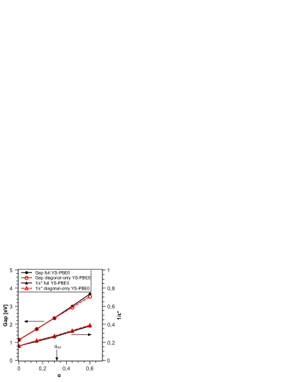
Figure 6: (Color online) Dependence of the band gap and the inverse dielectric constant on the amount of HF exchange in full and diagonal YS-PBE0 in CdS. Lines are a guide to the eye.

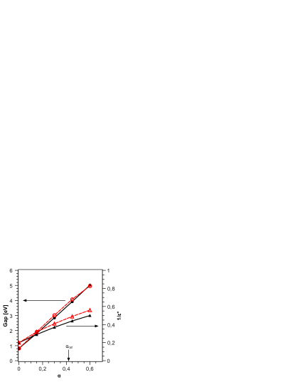
Figure 7: (Color online) Dependence of the band gap and the inverse dielectric constant on the amount of HF exchange in full and diagonal YS-PBE0 in ZnO. Lines are a guide to the eye.

In order to analyze why this scheme works for most cases but has some exceptions, we take a closer look at CdS as an example for a working case and at ZnO as an example for an exception. The relevant data are shown in Figs. 6 and 7. We can see that in both cases the dependency of the band gaps on $\alpha$ using the full hybrid or the diagonal-hybrid approximation is nearly identical and fairly linear. For CdS the same holds for the dependency of $1/\varepsilon^{*}$ on $\alpha$. However, for ZnO there is a substantial difference between the dielectric constant obtained with full hybrid calculations and that obtained with the diagonal approximation. The reason for that is that in the diagonal calculations only the eigenvalues change (to almost the same values as in full hybrid calculations), but the orbitals do not and still belong to the single-particle Hamiltonian with a semilocal potential. While in the case of CdS the eigenfunctions from PBE or full hybrid-DFT calculations do not differ much so that the dielectric constants with these two schemes remain very similar, in the case of ZnO there is a strong difference in the eigenfunctions from PBE or hybrid-DFT. This leads to different momentum matrix elements and therefore dielectric constants and finally the band gaps differ substantially.

IV Summary and Conclusion

A hybrid functional was presented which, in contrast to most currently established hybrid functionals, uses a HF mixing parameter which is individually adapted for each investigated system. This is achieved automatically using the calculated dielectric constant. Since this is a global quantity of a bulk material, the functional as described here can be applied reasonably only to systems with strict 3-dimensional periodicity. However it may be generalized in the course of future work so that defect structures, molecules, surfaces and interfaces can be dealt with. Actually, it has been claimedJain et al. (2011) that a hybrid functional with position-independent mixing factor and screening length is not appropriate for such cases.

The results obtained with this functional are quite impressive. Band gaps for a wide range of materials are much better reproduced than by hybrid functionals with a fixed parameter. Structural properties, which are usually not considered in similar studies, are in most cases of excellent quality and only in highly ionic insulators problems appear. However, even in these cases, good results can be obtained when one fixes $\alpha_{\text{opt}}$ at one volume and neglects its volume variations.

We have also tested an approximate version of this approach, namely a non self-consistent hybrid scheme considering only the diagonal HF matrix elements. Except for transition metal oxides (where even non self-consistent $GW$ methods fail) this approach leads to almost identical band gaps and such a method can be used to predict reliable band gaps in systems with hundreds of atoms.