Modeling temporal gradients in regionally aggregated California asthma hospitalization data

Abstract

Advances in Geographical Information Systems (GIS) have led to the enormous recent burgeoning of spatial-temporal databases and associated statistical modeling. Here we depart from the rather rich literature in space–time modeling by considering the setting where space is discrete (e.g., aggregated data over regions), but time is continuous. Our major objective in this application is to carry out inference on gradients of a temporal process in our data set of monthly county level asthma hospitalization rates in the state of California, while at the same time accounting for spatial similarities of the temporal process across neighboring counties. Use of continuous time models here allows inference at a finer resolution than at which the data are sampled. Rather than use parametric forms to model time, we opt for a more flexible stochastic process embedded within a dynamic Markov random field framework. Through the matrix-valued covariance function we can ensure that the temporal process realizations are mean square differentiable, and may thus carry out inference on temporal gradients in a posterior predictive fashion. We use this approach to evaluate temporal gradients where we are concerned with temporal changes in the residual and fitted rate curves after accounting for seasonality, spatiotemporal ozone levels and several spatially-resolved important sociodemographic covariates.

, and

1 Introduction

Technological advances in spatially-enabled sensor networks and geospatial information storage, analysis and distribution systems have led to a burgeoning of spatial-temporal databases. Accounting for associations across space and time constitutes a routine component in analyzing geographically and temporally referenced data sets. The inference garnered through these analyses often supports decisions with important scientific implications, and it is therefore critical to accurately assess inferential uncertainty. The obstacle for researchers is increasingly not access to the right data, but rather implementing appropriate statistical methods and software.

There is a considerable literature in spatio-temporal modeling; see, for example, the recent book by Cressie and Wikle (2011) and the references therein. Space–time modeling can broadly be classified as considering one of the following four settings: (a) space is viewed as continuous, but time is taken to be discrete, (b) space and time are both continuous, (c) space and time are both discrete, and (d) space is viewed as discrete, but time is taken to be continuous. Almost exclusively, the existing literature considers the first three settings. Perhaps the most pervasive case is the first. Here, the data are regarded as a time series of spatial process realizations. Early approaches include the STARMA [Pfeifer and Deutsch (1980a, 1980b)] and STARMAX [Stoffer (1986)] models, which add spatial covariance structure to standard time series models. Handcock and Wallis (1994) employ stationary Gaussian process models with an $\operatorname{AR}(1)$ model for the time series at each location to study global warming. Building upon previous work in the setting of dynamic models by West and Harrison (1997), several authors, including Stroud, Müller and Sansó (2001) and Gelfand, Banerjee and Gamerman (2005), proposed dynamic frameworks to model residual spatial and temporal dependence.

When space and time are both viewed as continuous, the preferred approach is to construct stochastic processes using space–time covariance functions. Gneiting (2002) built upon earlier work by Cressie and Huang (1999) to propose general classes of nonseparable, stationary covariance functions that allow for space–time interaction terms for spatiotemporal random processes. Stein (2005) considered a variety of properties of space–time covariance functions and how these were related to process spatial-temporal interactions.

Finally, in settings where both space and time are discrete there has been much spatiotemporal modeling based on a Markov random field (MRF) structure in the form of conditionally autoregressive (CAR) specifications. See, for example, Waller et al. (1997), who developed such models in the service of disease mapping, and Gelfand et al. (1998), whose interest was in single family home sales. Pace et al. (2000) work with simultaneous autoregressive (SAR) models extending them to allow temporal neighbors as well as spatial neighbors. Later examples include the space–time interaction CAR model proposed by Schmid and Held (2004), the dynamic CAR model proposed by Martínez-Beneito, López-Quilez and Botella-Rocamora (2008), the proper Gaussian MRF process models of Vivar and Ferreira (2009) and the latent structure models approach from Lawson et al. (2010).

Our manuscript departs from this rich literature by considering the setting where space is discrete and time is continuous. This can be envisioned when, for instance, we have a collection of $N_{s}$ functions of time over $N_{s}$ regions, but the functions are posited to be spatially associated. That is, functions arising from neighboring regions are believed to resemble each other. The functional data analysis literature [Ramsay and Silverman (1997) and references therein] deals almost exclusively with kernel smoothers and roughness-penalty type (spline) models; recent discrete-space, continuous time examples using spline-based methods include the works by MacNab and Gustafson (2007) and Ugarte, Goicoa and Militino (2010). Baladandayuthapani et al. (2008) consider spatially correlated functional data modeling for point-referenced data by treating space as continuous. A recent review by Delicado et al. (2010) reveals that spatially associated functional modeling of time has received little attention, especially for regionally aggregated data. This is unfortunate, especially given the data set we encounter here (see Section 2 below).

As such, we propose a rich class of Bayesian space–time models based upon a dynamic MRF that evolves continuously over time. This accommodates spatial processes that are posited to be spatially indexed over a geographical map with a well-defined system of neighbors. This continuous temporal evolution sets our current article apart from the existing literature. Rather than modeling time using simple parametric forms, as is often done in longitudinal contexts, we employ a stochastic process, enhancing the model’s adaptability to the data.

The benefits of using a continuous-time model over a discrete-time model here are twofold. First and foremost, investigators (or, in our setting, public health officials) may desire understanding of the local effects of temporal impact at a resolution finer than that at which the data were sampled. For instance, despite collecting data monthly, there may be interest in making inference on a particular week or even a given day of that month. While there is a wealth of literature in this domain, dynamic space–time models that treat time discretely can offer statistically legitimate inference only at the level of the data. Second, the modeling also allows us to subsequently carry out inference on temporal gradients, that is, the rate of change of the underlying process over time. We show how such inference can be carried out in fully model-based fashion using exact posterior predictive distributions for the gradients at any arbitrary time point.

The smoothness implications for the underlying process in this context are obvious. We deploy a mean square differentiable Gaussian process that provides a tractable gradient (or derivative) process to help us achieve these inferential goals. Here our goal is to detect temporal changes in the residuals that remain after accounting for important covariates; significant changes may correspond to changes in spatiotemporal covariates still missing from our model. While the residuals themselves could be beneficial in detecting missing covariates, temporal gradients can be more useful in detecting covariates that operate on much finer scales. For example, time points with significantly high residual gradients are likely to point toward missing covariates whose rapid changes on a finer scale impact the outcome. On the other hand, the residual process estimated from discrete time models is likely to smooth over any patterns arising from such local behavior of covariates.

The remainder of the manuscript is structured as follows. Section 2 describes the data set that motivates our methodology and which we analyze in depth. Section 3 outlines a class of dynamic MRF indexed continuously over time. Section 4 provides details on the Bayesian hierarchical models that emerge from our rich space–time structures, while Section 5 derives the posterior predictive inferential procedure for the temporal gradient process, verified via simulation in Section 6. Section 7 describes the detailed analysis of our data set, while Section 8 summarizes and concludes.

2 Data

Our data set consists of asthma hospitalization rates in the state of California. According to the California Department of Health Services (2003), millions of residents of California suffer from asthma or asthma-like symptoms. As many studies have indicated [e.g., English et al. (1998)], asthma rates are related to, among other things, pollution levels and socioeconomic status (SES)—two variables that likely induce a spatiotemporal distribution on such rates. Weather and climate also likely play a role, as cold air can trigger asthma symptoms.

The data we will analyze were collected daily from 1991 to 2008 from each of the 58 counties. We consider all hospital discharges where asthma was the primary diagnosis, which are categorized as extrinsic (allergic), intrinsic (nonallergic) or other. Due to confidentiality, data for days with between one and four hospitalizations of a specific category are missing; this affected 38% of our observations, including more than 50% of those from 21 counties. To remedy this, county-specific values for these days are imputed using a method similar to Besag’s iterated conditional modes method [Besag (1986)]; see the online supplement [Quick, Banerjee and Carlin (2013)] for details. For our analysis, the data are aggregated by month, for a total of 216 observations per county over the 18-year period, and then rates per 100,000 residents are computed; the conversion from counts to rates for the purpose of fitting Gaussian spatiotemporal models is common in the literature [see, e.g., Short, Carlin and Bushhouse (2002)]. While the vast majority of rates are less than 20 hospitalizations per month per 100,000 people, the range of the rates extends from 0 to 90. As can be seen in Figure 1, hospitalization for asthma demonstrates a statewide decreasing trend early in the study period and appears to stabilize in later years. Here, we map the raw annual (summed over month) hospitalization rates, which have values between 0 and 340 hospitalizations per 100,000.

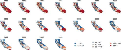
Figure 1: Raw annual (summed over month) asthma hospitalization rates per 100,000. Note: the analysis performed here was conducted on the monthly level; annual aggregation for illustration purposes only.

We attempt to capture the effect of socioeconomic status by including population density in our model, using data from the 2000 U.S. Census and land area measurements from the National Association of Counties. To account for pollution, we use data from the Air Resources Board of the California Environmental Protection Agency which counts the number of days in each month with average ozone levels above 0.07 ppm over 8 consecutive hours, the state standard. Because our ozone data is compiled at the air basin level, county-specific values are calculated by taking the maximum value of all air basins that the county belonged to. Generally, ozone levels are highest during the summer months, with the highest values in southern California and the Central Valley region, and show little variation between years. As hospitalization rates are higher among youth and the black population, county-level covariates for percent under 18 and percent black are also included. These demographic covariates both have their highest values in southern California, though counties in the Central Valley region also have larger black populations.

3 Areally referenced temporal processes

As mentioned above, ourmethodological contribution is a modeling framework for areally referenced outcomes that, it can be reasonably assumed, arise from an underlying stochastic process continuous over time. To be specific, consider a map of a geographical region comprising $N_{s}$ regions that are delineated by well-defined boundaries, and let $Y_{i}(t)$ be the outcome arising from region $i$ at time $t$. For every region $i$, we believe that $Y_{i}(t)$ exists, at least conceptually, at every time point. However, the observations are collected not continuously but at discrete time points, say, $\mathcal{T}=\{t_{1},t_{2},\ldots,t_{N_{t}}\}$. For the time being, we will assume that the data comes from the same set of time points in $\mathcal{T}$ for each region. This is not necessary for the ensuing development, but will facilitate the notation.

A spatial random effect model for our data assumes

$$Y_{i}(t)=\mu_{i}(t)+Z_{i}(t)+\varepsilon_{i}(t),\qquad\varepsilon_{i}(t)\stackrel{{\scriptstyle\mathrm{ind}}}{{\sim}}N\bigl{(}0,\tau_{i}^{2}\bigr{)}$$

(1)

$$\eqntext{\mbox{for }i=1,2,\ldots,N_{s},}$$ (2)

where $\mu_{i}(t)$ captures large scale variation or trends, for example, using a regression model, and $Z_{i}(t)$ is an underlying areally-referenced stochastic process over time that captures smaller-scale variations in the time scale while also accommodating spatial associations. Each region also has its own variance component, $\tau_{i}^{2}$, which captures residual variation not captured by the other components.

The process $Z_{i}(t)$ specifies the probability distribution of correlated space–time random effects while treating space as discrete and time as continuous. We seek a specification that will allow temporal processes from neighboring regions to be more alike than from nonneighbors. As regards spatial associations, we will respect the discreteness inherent in the aggregated outcome. Rather than model an underlying response surface continuously over the region of interest, we want to treat the $Z_{i}(t)$’s as functions of time that are smoothed across neighbors.

The neighborhood structure arises from a discrete topology comprising a list of neighbors for each region. This is described using an $N_{s}\times N_{s}$ adjacency matrix $W=\{w_{ij}\}$, where $w_{ij}=0$ if regions $i$ and $j$ are not neighbors and $w_{ij}=c\neq 0$ when regions $i$ and $j$ are neighbors, denoted by $i\sim j$. By convention, the diagonal elements of $W$ are all zero. To account for spatial association in the $Z_{i}(t)$’s, a temporally evolving MRF for the areal units at any arbitrary time point $t$ specifies the full conditional distribution for $Z_{i}(t)$ as depending only upon the neighbors of region $i$,

$$p\bigl{(}Z_{i}(t)|\bigl{\{}Z_{j\neq i}(t)\bigr{\}}\bigr{)}\sim N\biggl{(}\sum_{j\sim i}\alpha\frac{w_{ij}}{w_{i+}}Z_{j}(t),\frac{\sigma^{2}}{w_{i+}}\biggr{)},$$ (3)

where $w_{i+}=\sum_{j\sim i}w_{ij}$, $\sigma^{2}>0$, and $\alpha$ is a propriety parameter described below. This means that the $N_{s}\times 1$ vector $\mathbf{Z}(t)=(Z_{1}(t),Z_{2}(t),\ldots,Z_{N_{s}}(t))^{T}$ follows a multivariate normal distribution with zero mean and a precision matrix $\frac{1}{\sigma^{2}}(D-\alpha W)$, where $D$ is a diagonal matrix with $w_{i+}$ as its $i$th diagonal elements. The precision matrix is invertible as long as $\alpha\in(1/\lambda_{(1)},1/\lambda_{(n)})$, where $\lambda_{(1)}$ (which can be shown to be negative) and $\lambda_{(n)}$ (which can be shown to be 1) are the smallest (i.e., most negative) and largest eigenvalues of $D^{-1/2}WD^{-1/2}$, respectively, and this yields a proper distribution for $\mathbf{Z}(t)$ at each time point $t$.

The MRF in (3) does not allow temporal dependence; the $\mathbf{Z}(t)$’s are independently and identically distributed as $N(\mathbf{0},\sigma^{2}(D-\alpha W)^{-1})$. We could allow time-varying parameters $\sigma_{t}^{2}$ and $\alpha_{t}$ so that $\mathbf{Z}(t)\stackrel{{\scriptstyle\mathrm{ind}}}{{\sim}}N(\mathbf{0},\sigma_{t}^{2}(D-\alpha_{t}W)^{-1})$ for every $t$. If time were treated discretely, then we could envision dynamic autoregressive priors for these time-varying parameters, or some transformations thereof. However, there are two reasons why we do not pursue this further. First, we do not consider time as discrete because that would preclude inference on temporal gradients, which, as we have mentioned, is a major objective here. Second, time-varying hyperparameters, especially the $\alpha_{t}$’s, in MRF models are usually weakly identified by the data; they permit very little prior-to-posterior learning and often lead to over-parametrized models that impair predictive performance over time.

Here we prefer to jointly build spatial-temporal associations into the model using a multivariate process specification for $\mathbf{Z}(t)$. A highly flexible and computationally tractable option is to assume that $\mathbf{Z}(t)$ is a zero-centered multivariate Gaussian process, $\operatorname{GP}(\mathbf{0},K_{Z}(\cdot,\cdot))$, where the matrix-valued covariance function [e.g., “cross-covariance matrix function,” Cressie (1993)] $K_{Z}(t,u)=\operatorname{cov}\{\mathbf{Z}(t),\mathbf{Z}(u)\}$ is defined to be the $N_{s}\times N_{s}$ matrix with $(i,j)$th entry $\operatorname{cov}\{Z_{i}(t),Z_{j}(u)\}$ for any $(t,u)\in\Re^{+}\times\Re^{+}$. Thus, for any two positive real numbers $t$ and $u$, $K_{Z}(t,u)$ is an $N_{s}\times N_{s}$ matrix with $(i,j)$th element given by the covariance between $Z_{i}(t)$ and $Z_{j}(u)$. These multivariate processes are stationary when the covariances are functions of the separation between the time points, in which case we write $K_{Z}(t,u)=K_{Z}(\Delta)$, and fully symmetric when $K_{Z}(t,u)=K_{Z}(|\Delta|)$, where $\Delta=t-u$. For a detailed exposition on covariance functions, see Chapter 7 of Banerjee, Gelfand and Sirmans (2003); Gelfand and Banerjee (2010) and Gneiting and Guttorp (2010) also provide overviews for continuous settings.

To ensure valid joint distributions for process realizations, we use a constructive approach similar to that used in linear models of coregionalization (LMC) and, more generally, belonging to the class of multivariate latent process models [see Section 7.2 of Banerjee, Gelfand and Sirmans (2003)]. We assume that $\mathbf{Z}(t)$ arises as a (possibly temporally-varying) linear transformation $\mathbf{Z}(t)=A(t)\mathbf{v}(t)$ of a simpler process $\mathbf{v}(t)=(v_{1}(t),v_{2}(t),\ldots,v_{N_{s}}(t))^{T}$, where the $v_{i}(t)$’s are univariate temporal processes, independent of each other, and with unit variances. This differs from the conventional LMC approach based on spatial processes, which treats space as continuous. The matrix-valued covariance function for $\mathbf{v}(t)$, say, $K_{\mathbf{v}}(t,u)$, thus has a simple diagonal form and $K_{Z}(t,u)=A(t)K_{\mathbf{v}}(t,u)A(u)^{T}$. The dispersion matrix for $\mathbf{Z}$ is $\Sigma_{Z}=\mathcal{A}\Sigma_{\mathbf{v}}\mathcal{A}^{T}$, where $\mathcal{A}$ is a block-diagonal matrix with $A(t_{j})$’s as blocks, and $\Sigma_{\mathbf{v}}$ is the dispersion matrix constructed from $K_{\mathbf{v}}(t,u)$. Constructing simple valid matrix-valued covariance functions for $\mathbf{v}(t)$ automatically ensures valid probability models for $\mathbf{Z}(t)$. Also note that for $t=u$, $K_{\mathbf{v}}(t,t)$ is the identity matrix so that $K_{Z}(t,t)=A(t)A(t)^{T}$ and $A(t)$ is a square-root (e.g., obtained from the triangular Cholesky factorization) of the matrix-valued covariance function at time $t$.

The above framework subsumes several simpler and more intuitive specifications. One particular specification that we pursue here assumes that each $v_{i}(t)$ follows a stationary Gaussian Process $\operatorname{GP}(0,\rho(\cdot,\cdot;\bolds{\phi}))$, where $\rho(\cdot,\cdot;\phi)$ is a positive definite correlation function parametrized by $\bolds{\phi}$ [e.g., Stein (1999)], so that $\operatorname{cov}(v_{i}(t),v_{i}(u))=\rho(t,u;\phi)$ for every $i=1,2,\ldots,N_{s}$ for all nonnegative real numbers $t$ and $u$. Since the $v_{i}(t)$ are independent across $i$, $\operatorname{cov}\{v_{i}(t),v_{j}(u)\}=0$ for $i\neq j$.

The matrix-valued covariance function for $\mathbf{Z}(t)$ becomes $K_{Z}(t,u)=\rho(t,u;\break\bolds{\phi})A(t)A(u)^{T}$. If we further assume that $A(t)=A$ is constant over time, then the process $\mathbf{Z}(t)$ is stationary if and only if $\mathbf{v}(t)$ is stationary. Further, we obtain a separable specification, so that $K_{Z}(t,u)=\rho(t,u;\bolds{\phi})AA^{T}$. Letting $A$ be some square-root (e.g., Cholesky) of the $N_{s}\times N_{s}$ dispersion matrix $\sigma^{2}(D-\alpha W)^{-1}$ and $R(\bolds{\phi})$ be the $N_{t}\times N_{t}$ temporal correlation matrix having $(i,j)$th element $\rho(t_{i},t_{j};\bolds{\phi})$ yields

$$K_{Z}(t,u) = \sigma^{2}\rho(t,u;\bolds{\phi})(D-\alpha W)^{-1}\quad\mbox{and}$$

$$\Sigma_{Z} = R(\bolds{\phi})\otimes\sigma^{2}(D-\alpha W)^{-1}.$$

It is straightforward to show that the marginal distribution from this constructive approach for each $\mathbf{Z}(t_{i})$ is $N(\mathbf{0},\sigma^{2}(D-\alpha W)^{-1})$, the same marginal distribution as the temporally independent MRF specification in (3). Therefore, our constructive approach ensures a valid space–time process, where associations in space are modeled discretely using a MRF, and those in time through a continuous Gaussian process.

This separable specification is easily interpretable, as it factorizes the dispersion into a spatial association component (areal) and a temporal component. Another significant practical advantage is its computational feasibility. Estimating more general space–time models usually entails matrix factorizations with $O(N_{s}^{3}N_{t}^{3})$ computational complexity. The separable specification allows us to reduce this complexity substantially by avoiding factorizations of $N_{s}N_{t}\times N_{s}N_{t}$ matrices. One could design algorithms to work with matrices whose dimension is the smaller of $N_{s}$ and $N_{t}$, thereby accruing massive computational gains.

More general models using this approach are introduced and discussed in the online supplement [Quick, Banerjee and Carlin (2013)], but since they do not offer anything new in terms of temporal gradients, we do not pursue them in the remainder of this paper.

4 Hierarchical modeling

In this section we build a hierarchical modeling framework to analyze the data in Section 2 using the likelihood from our spatial random effects model in (3) and the distributions emerging from the temporal Gaussian process discussed in Section 3. The mean $\mu_{i}(t)$ in (3) is often indexed by a parameter vector $\bolds{\beta}$, for example, a linear regression with regressors indexed by space and time so that $\mu_{i}(t;\bolds{\beta})=\mathbf{x}_{i}(t)^{T}\bolds{\beta}$.

The posterior distributions we seek can be expressed as

$$p(\bolds{\theta},\mathbf{Z}|\mathbf{Y}) \propto p(\bolds{\phi})\times\operatorname{IG}\bigl{(}\sigma^{2}|a_{\sigma},b_{\sigma}\bigr{)}\times\Biggl{(}\prod_{i=1}^{M}\operatorname{IG}\bigl{(}\tau_{i}^{2}|a_{\tau},b_{\tau}\bigr{)}\Biggr{)}\times N(\bolds{\beta}|\mu_{\beta},\Sigma_{\beta})$$

$${}\times\operatorname{Beta}(\alpha|a_{\alpha},b_{\alpha})$$

$${}\times N\bigl{(}\mathbf{Z}|\mathbf{0},R(\phi)\otimes\sigma^{2}(D-\alpha W)^{-1}\bigr{)}$$

$${}\times\prod_{j=1}^{N_{t}}\prod_{i=1}^{N_{s}}N\bigl{(}Y_{i}(t_{j})|\mathbf{x}_{i}(t_{j})^{T}\bolds{\beta}+Z_{i}(t_{j}),\tau_{i}^{2}\bigr{)},$$

where $\bolds{\theta}=\{\bolds{\phi},\alpha,\sigma^{2},\bolds{\beta},\tau_{1}^{2},\tau_{2}^{2},\ldots,\tau_{N_{s}}^{2}\}$ and $\mathbf{Y}$ is the vector of observed outcomes defined analogous to $\mathbf{Z}$. The parametrizations for the standard densities are as in Carlin and Louis (2009). We assume all the other hyperparameters in (4) are known.

Recall the separable matrix-valued covariance function in (3). The correlation function $\rho(\cdot;\bolds{\phi})$ determines process smoothness and we choose it to be a fully symmetric Matérn correlation function given by

$$\qquad\rho(t,u;\bolds{\phi})=\rho(\Delta;\bolds{\phi})=\frac{1}{\Gamma(\phi_{2})2^{\phi_{2}-1}}\bigl{(}2\sqrt{\phi_{2}}|\Delta|\phi_{1}\bigr{)}^{\phi_{2}}\mathcal{K}_{\phi_{2}}\bigl{(}2\sqrt{\phi_{2}}|\Delta|\phi_{1}\bigr{)},$$ (6)

where $\bolds{\phi}=\{\phi_{1},\phi_{2}\}$, $\Delta=t-u$, $\Gamma(\cdot)$ is the Gamma function, $\mathcal{K}_{\phi_{2}}(\cdot)$ is the modified Bessel function of the second kind, and $\phi_{1}$ and $\phi_{2}$ are nonnegative parameters representing rate of decay in temporal association and smoothness of the underlying process, respectively.

We use Markov chain Monte Carlo (MCMC) to evaluate the joint posterior in (4), using Metropolis steps for updating $\bolds{\phi}$ and Gibbs steps for all other parameters, details of which are shown in the supplemental article [Quick, Banerjee and Carlin (2013)]. Sampling-based Bayesian inference seamlessly delivers inference on the residual spatial effects. Specifically, if $t_{0}$ is an arbitrary unobserved time point, then, for any region $i$, we sample from the posterior predictive distribution $p(Z_{i}(t_{0})|\mathbf{Y})=\int p(Z_{i}(t_{0})|\mathbf{Z},\bolds{\theta})p(\bolds{\theta},\break\mathbf{Z}|\mathbf{Y})\,d\bolds{\theta}\,d\mathbf{Z}$. This is achieved using composition sampling: for each sampled value of $\{\bolds{\theta},\mathbf{Z}\}$, we draw $Z_{i}(t_{0})$, one for one, from $p(Z_{i}(t_{0})|\mathbf{Z},\bolds{\theta})$, which is Gaussian. Also, our sampler easily adapts to situations where $Y_{i}(t)$ is missing (or not monitored) for some of the time points in region $i$. We simply treat such variables as missing values and update them, from their associated full conditional distributions, which of course are $N(\mathbf{x}_{i}(t)^{T}\bolds{\beta}+Z_{i}(t),\tau^{2}_{i})$. We assume that all predictors in $\mathbf{x}_{i}(t)$ will be available in the space–time data matrix, so this temporal interpolation step for missing outcomes is straightforward and inexpensive.

Model checking is facilitated by simulating independent replicates for each observed outcome: for each region $i$ and observed time point $t_{j}$, we sample from $p(Y_{\mathrm{rep},i}(t_{j})|\mathbf{Y})=\int N(Y_{\mathrm{rep},i}(t_{j})|\mathbf{x}_{i}(t_{j})^{T}\bolds{\beta}+Z_{i}(t_{j}),\tau_{i}^{2})p(\bolds{\beta},Z_{i}(t_{j}),\break\tau_{i}^{2}|\mathbf{Y})\,d\bolds{\beta}\,dZ_{i}(t_{j})\,d\tau_{i}^{2}$, where $p(\bolds{\beta},Z_{i}(t_{j}),\tau_{i}^{2}|\mathbf{Y})$ is the marginal posterior distribution of the unknowns in the likelihood. Sampling from the posterior predictive distribution is straightforward, again, using composition sampling.

5 Gradient analysis

Our primary goal is to carry out statistical inference on temporal gradients with data arising from a temporal process indexed discretely over space. We will do so using the notions of smoothness of a Gaussian process and its derivative. Adler (2009), Mardia et al. (1996) and Banerjee and Gelfand (2003) discuss derivatives (more generally, linear functionals) of Gaussian processes, while Banerjee, Gelfand and Sirmans (2003) lay out an inferential framework for directional gradients on a spatial surface. Most of the existing work on derivatives of stochastic processes deal either with purely temporal or purely spatial processes [see, e.g., Banerjee (2010)]. Here, we consider gradients for a temporal process indexed discretely over space.

Assume that $\{Z_{i}(t)\dvtx t\in{\Re^{+}}\}$ is a stationary random process for each region $i$. The process is $L_{2}$ (or mean square) continuous at $t_{0}$ if $\mathop{\lim}_{t\rightarrow t_{0}}E|Z_{i}(t)-Z_{i}(t_{0})|^{2}=0$. The notion of a mean square differentiable process can be formalized using the analogous definition of total differentiability of a function in a nonstochastic setting [see, e.g., Banerjee and Gelfand (2003)]: $Z_{i}(t)$ is mean square differentiable at $t_{0}$ if it admits a first order linear expansion for any scalar $h$,

$$Z_{i}(t_{0}+h)=Z_{i}(t_{0})+hZ_{i}^{\prime}(t)+o(h)$$ (7)

in the $L_{2}$ sense as $h\rightarrow 0$, where we say that $\frac{d}{dt}Z_{i}(t)=Z_{i}^{\prime}(t_{0})$ is the gradient or derivative process derived from the parent process $Z_{i}(t)$. In other words, we require

$$\mathop{\lim}_{h\rightarrow 0}E\biggl{(}\frac{Z_{i}(t_{0}+h)-Z_{i}(t_{0})}{h}-Z_{i}^{\prime}(t_{0})\biggr{)}^{2}=0.$$ (6^′)

Equations (7) and (6^′) ensure that mean square differentiable processes are mean square continuous.

For a univariate stationary process, smoothness in the mean square sense is determined by its covariance or correlation function. A stationary multivariate process $\mathbf{Z}(t)$ with matrix-valued covariance function $K_{Z}(\Delta)$ will admit a well-defined gradient process $\mathbf{Z}^{\prime}(t)=(Z_{1}^{\prime}(t),\ldots,Z_{N_{s}}^{\prime}(t))^{T}$ if and only if $K_{Z}^{\prime\prime}(0)$ exists, where $K_{Z}^{\prime\prime}(0)$ is the element-wise second-derivative of $K_{Z}(\Delta)$ evaluated at $\Delta=0$.

A Gaussian process with a Matérn correlation function has sample paths that are $\lceil\phi_{2}-1\rceil$ times differentiable. As $\phi_{2}\to\infty$, the Matérn correlation function converges to the squared exponential (or the so-called Gaussian) correlation function, which is infinitely differentiable and leads to acute oversmoothing. When $\phi_{2}=0.5$, the Matérn correlation function is identical to the exponential correlation function [see, e.g., Stein (1999)]. To ensure that the underlying process is differentiable so that the gradient process exists, we need to restrict $\phi_{2}>1$. However, letting $\phi_{2}>2$ usually leads to oversmoothing, as the data can rarely distinguish among values of the smoothness parameter greater than $2$. Hence, we restrict $\phi_{2}\in(1,2]$. We could either assign a prior on this support or simply fix $\phi_{2}$ somewhere in this interval. Since it is difficult to elicit informative priors for the smoothness parameter, we would most likely end up with a uniform prior. In our experience, not only does this deliver only modest posterior learning and lead to an increase in computing (both in terms of MCMC convergence and estimating the resulting correlation function and its derivative), but the substantive inference is almost indistinguishable from what is obtained by fixing $\phi_{2}$.

As such, in our subsequent analysis we fix $\phi_{2}=3/2$, which has the side benefit of yielding the closed form expression $\rho(\Delta;\phi_{1})=(1+\phi_{1}|\Delta|)\times\break\exp(-\phi_{1}|\Delta|)$. The first and second order derivatives for the matrix-valued covariance function in (3) can now be obtained explicitly as

$$K_{Z}^{\prime}(\Delta) = -\sigma^{2}\phi_{1}^{2}\Delta\exp\bigl{(}-\phi_{1}|\Delta|\bigr{)}(D-\alpha W)^{-1}\quad\mbox{and}$$

$$-K_{Z}^{\prime\prime}(0) = \sigma^{2}\phi_{1}^{2}(D-\alpha W)^{-1}.$$

Turning to inference for gradients, we seek the joint posterior predictive distribution,

$$p\bigl{(}\mathbf{Z}^{\prime}(t_{0})|\mathbf{Y}\bigr{)} = \int p\bigl{(}\mathbf{Z}^{\prime}(t_{0})|\mathbf{Y},\mathbf{Z},\bolds{\theta}\bigr{)}p(\mathbf{Z}|\bolds{\theta},\mathbf{Y})p(\bolds{\theta}|\mathbf{Y})\,d\bolds{\theta}\,d\mathbf{Z}$$

$$= \int p\bigl{(}\mathbf{Z}^{\prime}(t_{0})|\mathbf{Z},\bolds{\theta}\bigr{)}p(\mathbf{Z}|\bolds{\theta},\mathbf{Y})p(\bolds{\theta}|\mathbf{Y})\,d\bolds{\theta}\,d\mathbf{Z},$$

where the second equality follows from the fact that the gradient process is derived entirely from the parent process and so $p(\mathbf{Z}^{\prime}(t_{0})|\mathbf{Y},\mathbf{Z},\bolds{\theta})$ does not depend on $\mathbf{Y}$.

We evaluate (5) using composition sampling. Here, we first obtain $\bolds{\theta}^{(1)},\bolds{\theta}^{(2)},\break\ldots,\bolds{\theta}^{(M)}\sim p(\bolds{\theta}|\mathbf{Y})$ and $\mathbf{Z}^{(j)}\sim p(\mathbf{Z}|\bolds{\theta}^{(j)},\mathbf{Y}),j=1,2,\ldots,M$, where $M$ is the number of (post-burn-in) posterior samples. Next, for each $j$ we draw $\mathbf{Z}^{(j)}\sim p(\mathbf{Z}|\bolds{\theta}^{(j)},\mathbf{Y})$, and finally $\mathbf{Z}^{\prime}(t_{0})^{(j)}\sim p(\mathbf{Z}^{\prime}(t_{0})|\mathbf{Z}^{(j)},\bolds{\theta}^{(j)})$. The conditional distribution for the gradient can be seen to be multivariate normal with mean and variance-covariance matrix given by

$$\bolds{\mu}_{Z^{\prime}|Z,\theta} = \operatorname{cov}\bigl{(}\mathbf{Z}^{\prime}(t_{0}),\mathbf{Z}\bigr{)}\operatorname{var}(\mathbf{Z})^{-1}\mathbf{Z}=-\bigl{(}K_{Z}^{\prime}\bigr{)}^{T}\Sigma_{Z}^{-1}\mathbf{Z}\quad\mbox{and}$$

$$\Sigma_{Z^{\prime}|Z,\theta} = -K_{Z}^{\prime\prime}(0)-\bigl{(}K_{Z}^{\prime}\bigr{)}^{T}\Sigma_{Z}^{-1}\bigl{(}K_{Z}^{\prime}\bigr{)},$$

where $\Sigma_{Z}^{-1}=\frac{1}{\sigma^{2}}R(\phi)^{-1}\otimes(D-\alpha W)$ and $(K_{Z}^{\prime})^{T}$ is an $N_{s}\times N_{s}N_{t}$ block matrix whose $j$th block is given by the $N_{s}\times N_{s}$ matrix $K_{Z}^{\prime}(\Delta_{0j})$, with $\Delta_{0j}=t_{j}-t_{0}$. Note that $\Sigma_{Z^{\prime}|Z,\theta}$ is an $N_{s}N_{t}\times N_{s}N_{t}$ matrix, but we can use the properties of the MRF to only invert $N_{t}\times N_{t}$ matrices.

6 Simulation studies

To validate our model’s ability to correctly estimate both our model parameters and the underlying temporal gradients, we have constructed two separate simulation studies using the $N_{s}=58$ counties of California as our spatial grid and $N_{t}=50$ observations per county, where $\mathcal{T}=\{1,2,\ldots,50\}$. Each simulation study consists of 100 data sets comprised of 2900 observations generated from (3), where $\mu_{i}(t)=\mathbf{x}_{i}(t)^{T}\bolds{\beta}$, using the same parameter values, and our results are based on 5000 MCMC samples after a burn-in period of 5000 iterations.

In an effort to obtain simulated outcomes comparable to those from our real data, our first simulation study uses an intercept and the four covariates described in Section 2, and we set the $5\times 1$ vector, $\bolds{\beta}$, as the least squares estimates from our real data. We also set $\phi=1$, $\alpha=0.90$, and $\sigma^{2}=18$, which are then used to generate true values for $\mathbf{Z}$, while our $\tau_{i}^{2}$ are drawn from an inverse Gamma distribution centered at 1 with modest variance. For each of the 100 simulated data sets, we constructed $95\%$ Bayesian credible intervals for each parameter and recorded the number of times they included their true values (i.e., their “frequentist coverage”). We found this coverage to be between 93–97% for the 5 $\beta$’s, about $87\%$ for the random effect variance $\sigma^{2}$ and around $90\%$ on the average for the $58$ $\tau_{i}^{2}$’s, with the majority of them having $95\%$ coverage. Coverage was poor for $\tau_{i}^{2}<0.15$; in situations where small variances are to be expected, this issue could be avoided or alleviated by rescaling the data or specifying a prior with a larger mass near 0, respectively. The spatiotemporal random effects, $\mathbf{Z}$, also enjoyed satisfactory coverage; the average coverage over the 2900 space–time random effects was around $95.5\%$. By contrast, the coverage for the propriety parameter, $\alpha$, and the spatial range parameter, $\phi$, reveal biases, with coverages less than $50\%$. This is not entirely unexpected, as spatial and temporal range parameters of this type are known to be weakly identified by the data [e.g., Zhang (2004)]. Furthermore, the biases for $\phi$ and $\alpha$ are not substantial, with their posterior medians only 8% above and 5% below their true values, respectively. In an effort to verify the robustness of our model to these biases, we repeated the simulation with both $\phi$ and $\alpha$ fixed at their true values and were able to reproduce our results.

Having demonstrated the ability of our model to correctly estimate model parameters, the focus of our second simulation study is to validate the theory of our temporal gradient processes. To do this, we assumed

$$Y_{i}(t_{j})\stackrel{{\scriptstyle{\mathrm{ind}}}}{{\sim}}N\biggl{(}5+x_{i1}*\operatorname{sin}\biggl{(}\frac{t_{j}}{2}\biggr{)}+x_{i2}*\operatorname{cos}\biggl{(}\frac{t_{j}}{2}\biggr{)},\tau_{i}^{2}\biggr{)},$$ (9)

where $x_{i1}$ is the $i$th county’s percent black and $x_{i2}$ is the $i$th county’s ozone level from April 1991, as described in Section 2; this was done in order to induce spatial clustering. As there was no evidence of an association between the coverage of the random effects, $\mathbf{Z}$, and the region-specific variance parameters, values of $\tau_{i}^{2}$ were generated from a $\operatorname{Uniform}(0.5,2.0)$ distribution in order to avoid the extreme values of the inverse Gamma and focus our attention on the random effects themselves. After generating 100 data sets based on these parameters, we then modeled the data using only an intercept, leaving the spatiotemporal random effects to capture the sinusoidal curve, and conducted the gradient analysis at the midpoints of each time interval. Figure 2 displays the true spatiotemporal random effects and temporal gradients for a particular region, along with their 95% CI estimated from one of the 100 data sets. As can be seen, our Gaussian process model accurately estimates both the random effects and the temporal gradients. Across all 100 data sets, 98.3% of the the theoretical gradients derived using elementary calculus were covered by their respective 95% CI, confirming the validity of the gradient theory derived in Section 5.

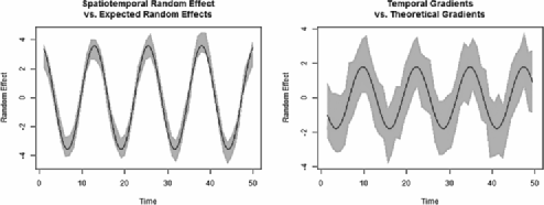
Figure 2: Spatiotemporal random effects and temporal gradients for a region based on one data set from the second simulation study. Solid black lines denote true sinusoidal curves based on the model in equation (9), while gray bands represent 95% credible intervals.

7 Data analysis

As first mentioned in Section 2, our data set is comprised of monthly asthma hospitalization rates in the counties of California over an 18-year period. As such, $N_{t}=12\cdot 18=216$, and we will again use $t_{j}=j=1,2,\ldots,N_{t}$. The covariates in this model include population density, ozone level, the percent of the county under 18 and percent black. Population-based covariates are calculated for each county using the 2000 U.S. Census, thus, they do not vary temporally. However, the covariate for ozone level is aggregated at the air basin level and varies monthly, though show little variation annually. In order to accommodate seasonality in the data, monthly fixed effects are included, using January as a baseline. Thus, after accounting for the monthly fixed effects and the four covariates of interest, $\mathbf{x}_{i}(t)$ is a $16\times 1$ vector.

To justify the use of the model we’ve described, we compare it to three alternative models using the DIC criterion [Spiegelhalter et al. (2002)] and a predictive model choice criterion using strictly proper scoring rules proposed by Gneiting and Raftery [(2007) equation (27)]. Following Czado, Gneiting and Held (2009), we refer to this as the Dawid–Sebastiani (D–S) score [Dawid and Sebastiani (1999)]. These models are all still of the form

$$Y_{i}(t)=\mathbf{x}_{i}(t)^{\prime}\bolds{\beta}+Z_{i}(t)+\varepsilon_{i}(t),\qquad\varepsilon_{i}(t)\stackrel{{\scriptstyle\mathrm{ind}}}{{\sim}}N\bigl{(}0,\tau_{i}^{2}\bigr{)}$$

(10)

$$\eqntext{\mbox{for }i=1,2,\ldots,N_{s},}$$ (11)

but with different $Z_{i}(t)$. Our first model is a simple linear regression model which ignores both the spatial and the temporal autocorrelation, that is, $Z_{i}(t)=0\ \forall i,t$. The second model allows for a random intercept and random temporal slope, but ignores the spatial nature of the data, that is, here $Z_{i}(t)=\alpha_{0i}+\alpha_{1i}t$, where $\alpha_{ki}\stackrel{{\scriptstyle{\mathrm{i.i.d.}}}}{{\sim}}N(0,\sigma_{k}^{2})$, for $k=0,1$. In this model, to preserve model identifiability, we must remove the global intercept from our design matrix, $\mathbf{x}_{i}(t)$. Our third model builds upon the second, but introduces spatial autocorrelation by letting $\bolds{\alpha}_{k}=(\alpha_{k1},\ldots,\alpha_{kN_{s}})^{\prime}\sim\operatorname{CAR}(\sigma_{k}^{2}),k=0,1$. The results of the model comparison can be seen in Table 1, which indicates that our Gaussian process model has the lowest DIC value and D–S score, and is thus the preferred model and the only one we consider henceforth. The surprisingly large $p_{D}$ for the areally referenced Gaussian process model arises due to the very large size of the data set (58 counties $\times$ 216 time points).

Table 1: Comparisons between our areally referenced Gaussian process model and the three alternatives. $p_{D}$ is a measure of model complexity, as it represents the effective number of parameters. Smaller values of DIC and Dawid–Sebastiani (D–S) scores indicate a better trade-off between in-sample model fit and model complexity

	$\bolds{p_{D}}$	DICt1	D–St1
Simple linear regression	0079	9894	16,166
Random intercept and slope	0165	4347	10,403
CAR model	0117	7302	13,436
Areally referenced Gaussian process	5256	0000	0000.0

[*]t1Both DIC and D–S shown are standardized relative to our areally referenced Gaussian Process model.

Table 2: Parameter estimates for asthma hospitalization data, where estimates for $\bar{\tau}_{\cdot}^{2}$ represent the median (95% CI) of the $\tau_{i}^{2},i=1,\ldots,N_{s}=58$

Parameter	Median (95% CI)	Parameter	Median (95% CI)
$\beta_{0}$ (Intercept)	9.17 (8.93, 9.42)0.	$\beta_{10}$ (July)	$-3.78$ ($-4.21$, $-3.37$)
$\beta_{1}$ (Pop Den)	0.60 (0.49, 0.70)0.	$\beta_{11}$ (August)	$-3.58$ ($-4.02$, $-3.13$)
$\beta_{2}$ (Ozone)	$-0.18$ ($-0.28$, $-0.08$)	$\beta_{12}$ (September)	$-1.96$ ($-2.37$, $-1.54$)
$\beta_{3}$ (% Black)	1.24 (1.15, 1.34)0.	$\beta_{13}$ (October)	$-1.36$ ($-1.73$, $-1.00$)
$\beta_{4}$ (% Under 18)	1.12 (1.01, 1.24)0.	$\beta_{14}$ (November)	$-0.71$ ($-1.02$, $-0.42$)
$\beta_{5}$ (February)	$-0.25$ ($-0.46$, $-0.04$)	$\beta_{15}$ (December)	0.63 (0.41, 0.86)0.
$\beta_{6}$ (March)	$-0.21$ ($-0.48$, 0.07)0.	$\phi$	0.90 (0.84, 0.97)0.
$\beta_{7}$ (April)	$-1.47$ ($-1.81$, $-1.12$)	$\alpha$	0.77 (0.71, 0.80)0.
$\beta_{8}$ (May)	$-1.17$ ($-1.53$, $-0.8$)0	$\sigma^{2}$	21.52 (20.18, 23.06).
$\beta_{9}$ (June)	$-2.79$ ($-3.21$, $-2.4$)0	$\bar{\tau}_{\cdot}^{2}$	.3.32 (0.18, 213.16)

The estimates for our model parameters can be seen in Table 2. The coefficients for the monthly covariates indicate decreased hospitalization rates in the summer months, a trend which is consistent with previous findings. The coefficients for population density, percent under 18 and percent black are all significantly positive, also as expected. The coefficient for ozone level is significantly negative, however, which is surprising but consistent with the patterns in the monthly trends for both hospitalization rates and ozone levels. This result may also be confounded by the absence of other climate-related factors and the sensitivity of asthma admissions to acute weather effects.

There is a large range of values for the county-specific residual variance parameters, $\tau_{i}^{2}$. Perhaps not surprisingly, the magnitude of these terms seems to be negatively correlated with the population of the given counties, demonstrating the effect a (relatively) small denominator can have when computing and modeling rates. The strong spatial story seen in the maps is reflected by the size of $\sigma^{2}$ compared to the majority of the $\tau_{i}^{2}$. There is also relatively strong temporal correlation, with $\phi=0.9$ corresponding to $\rho(t_{i},t_{j};\phi)\geq 0.4$ for $|t_{j}-t_{i}|$ less than 2 months.

Maps of the yearly (averaged across month) spatiotemporal random effects can be seen in Figure 3. Since here we are dealing with the residual curve after accounting for a number of mostly nontime-varying covariates, it comes as no surprise that the spatiotemporal random effects capture most of the variability in the model, including the striking decrease in yearly hospitalization rates over the study period. It also appears that our model is providing a better fit to the data in the years surrounding 2000, perhaps indicating that we could improve our fit by allowing our demographic covariates to vary temporally. Our model also appears to be performing well in the central counties, where asthma hospitalization rates remained relatively stable for much of the study period.

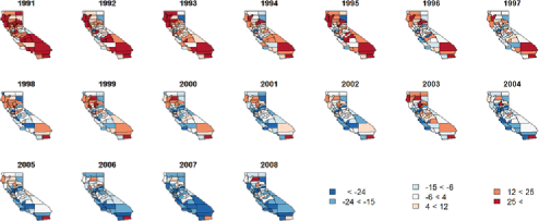
Figure 3: Spatial random effects for asthma hospitalization data, by year.

In the top panel of Figure 4, we compare the monthly temporal profiles of the random effects for Los Angeles and San Francisco Counties. For Los Angeles County, the spatiotemporal random effects (top-left panel) decrease at a consistent, moderate rate throughout the length of the study with several large spikes prior to 2000. In contrast, San Francisco County’s random effects (top-right) have fewer and less dramatic spikes. In addition, San Francisco County appears to have had a changepoint in its spatiotemporal random effects around 2000, where they transition from a fairly steady decline to a period of lower variability and very little mean change. Further investigation may reveal a corresponding change in social, environmental or health care reimbursement policy. The bottom-left panel shows the temporal trend of the gradients in Los Angeles County, which reveal the large degree of variability in the random effects. In fact, as more clearly shown in the bottom-right panel of Figure 4, the September to October gradient was significantly positive five times between 1995 and 2001, and three times during this period (1995, 1997 and 1999) the November to December gradients were significantly positive, but were immediately followed by significantly negative gradients from December to January, a pattern that is seen throughout the region.

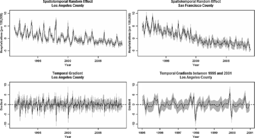
Figure 4: Comparison between the spatiotemporal random effects in Los Angeles and San Francisco Counties, and an investigation of temporal gradients in Los Angeles County. Point estimates in black and corresponding 95% CI bands in gray. Figures in the top panel illustrate the differences in the temporal trends of the random effects between the two counties. The bottom-left figure displays the temporal gradients computed between months in Los Angeles County, and the bottom-right figure displays the subset of the gradients which are further described in the text.

A strength of using a continuous-time model for these data is that it seamlessly permits prediction at a finer resolution than that of the observed data. Upon seeing the significant gradients in Los Angeles County in November and December of 1995, public health officials may ask for a more detailed report than a monthly aggregation can provide. If a discrete-time model were used, researchers would be required to refit the model, pre-specifying at which unobserved time points to conduct inference; however, with this model, we can use the posterior predictive distribution to interpolate values at any time. As a demonstration of this, Figure 5 displays the predicted daily values (solid line) and 95% CI bands (dashed lines) every 3 days during the period November 15, 1995 to January 15, 1996, plotted against the true observed rates (open circles). Despite substantial noise in the data and modeling based solely on the aggregate rates for each month (and assigning that value to the temporal midpoint of each month), our predictions and 95% CI bands perform reasonably well.

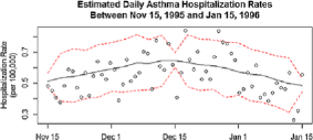
Figure 5: Posterior predicted curves (and 95% credible bounds) for the daily asthma hospitalization rates in Los Angeles County between November 15, 1995 to January 15, 1996. This county and interval was selected due the presence of a significantly positive gradient between November and December and a significantly negative gradient between December and January. The true hospitalizations are also shown for comparison purposes, though the model was fit using only the monthly aggregates.

As our data are aggregated monthly, we felt it was also important to investigate the gradients on a month-to-month basis over the course of the study. For instance, Figure 6 reveals the gradients between August and September decrease substantially statewide over the course of the study. Coupling this with the information in Table 2, which indicates that hospitalization rates in September are $\beta_{12}-\beta_{11}=1.62$ per 100,000 higher than those in August, suggests that the difference in asthma hospitalization rates between August and September has decreased nearly 60%, going from roughly 2.31 at the beginning of the period to just 0.97 by the end. An investigation of the raw hospitalization rates shows a similar trend, but this is to be expected since most of the spatiotemporal variability in the model is accounted for by the random effects. A similar, though not as striking, phenomenon occurs between March and April, where the gradients are increasing. As these two pairs of months lie on the transition between the warmer months and the cooler months, this result would seem to suggest that the effect of seasonality has moderated over the length of the study.

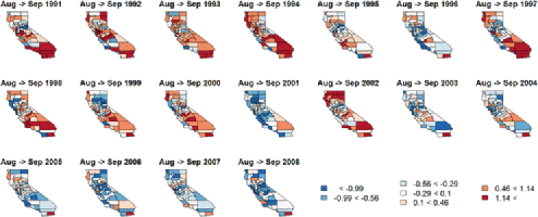
Figure 6: Temporal gradients for transition from August to September over time.

One limitation of this analysis is that the data records asthma hospitalizations, not overall prevalence. This is an important distinction, as factors that trigger symptoms of asthma may not be the same as or have the same impact on asthma hospitalizations. For instance, residents of regions with high risk environments may be better educated about and/or prepared for managing their symptoms, which could lead to a relative decrease in asthma hospitalization rates. Another limitation is that, due to the aggregation of our data, we have an inconvenient interpretation of the daily estimates in Figure 5. A more accurate interpretation of these values is that they are the average daily rates for the one-month interval centered at a particular day. More generally, the interpretation of predicted values at any time point is determined by the aggregation of the data, but this is certainly not unique to this model.

8 Summary and conclusions

In this paper we have provided an overview of parent and gradient processes, building on previous work in spatiotemporal Gaussian process modeling. We then described our modeling framework and methodology that allows for inference on temporal gradients. An implementation of this work was outlined in Section 4, and its theory was verified via simulation. Its use was then illustrated on a real data set in Section 7, where our results showed real insight can be gained from an assessment of temporal gradients in the residual Gaussian process, indicating overall trends as well as motivating a search for temporally interesting covariates still missing from our model (say, one that changes abruptly in San Francisco County around 2000).

We believe there are two primary points of discussion regarding this work, the first of which is the use of modeling time as continuous. If inference is desired at the resolution of the data only, then several of the discrete-time models in the literature would be appropriate; in Appendix D of the online supplement to this article, we compare our methods to one such model. Oftentimes, however, this is not the case, as investigators and administrators may seek estimates of the temporal effects on a finer scale. In our example, public health officials may be interested in the daily effects of asthma, which can be correlated with effects of daily variation of temperature and a variety of atmospheric pollutants. A practical issue here is that hospitalization data are often more cleanly available as monthly aggregates (say, due to patient confidentiality issues, like those described in Section 2) and, even when the daily data are available, they tend to be both massive and very likely to have many missing values. Analyzing such data using discrete-time models would require methods for handling temporal misalignment, while our temporal process-based methods can handle such inference in a posterior predictive fashion. Furthermore, treating time as continuous permits inference on temporal gradients, which we feel can be an important tool for better understanding complex space–time data sets. In some sense, our modeling framework can be looked upon as generalizing the work of Vivar and Ferreira (2009) with a stochastic temporal process and deriving a tractable inferential framework for infinitesimal rates of change for that process.

A second important point of discussion is the importance of significance with respect to these temporal gradients. We believe it depends on the problem being modeled. While we have accounted for monthly differences in our design matrix, the $Z_{i}(t)$ here may simply be capturing the remaining cyclical trend, and this is why we felt it was more beneficial to focus on a side-by-side comparison of two of California’s most populous counties, which motivated a further investigation of Los Angeles County, and the trends of the twelve month-to-month comparisons rather than solely on whether a specific gradient for a particular county was significant. In situations where it’s reasonable to assume two time points are comparable, investigating significant temporal gradients can indicate periods of important changes in the data, which may be caused by rapid changes in missing covariates. We also point out that the methodology for gradients outlined here can be applied to more general spatial functional data analysis contexts and will be especially useful for estimating gradients from high-resolution samples of the function.

Regarding the specific application of this methodology in this paper, it bears mentioning that modeling our data as rates is not the only option. Often, the counts themselves are modeled directly using a log-linear model, with a Poisson distributional assumption justified as a rare-events approximation to the binomial. In this setting, however, we would no longer be able to rely on the closed form Gibbs Sampler for updating our random effects, instead requiring Metropolis updates and a substantial increase in computational burden. Another option is to use a Freeman–Tukey transformation of the rates and a single error variance parameter, $\tau^{2}$, which is scaled by the county’s population, as shown in Freeman and Tukey (1950) and Cressie and Chan (1989), with the goal of justifying the assumption of normality. Given the population sizes we’re dealing with, we believe the assumption of normality of our observed rates can be justified as a normal approximation to the binomial. Furthermore, an analysis of the transformed data results in nearly identical substantive findings. However, there is a drawback: by modeling transformed values instead of the rates themselves, we lose the interpretability of the scale for not only our regression parameters, but also the temporal gradients. In our experience, a common question among public health practitioners is, “What does this mean?” As such, we feel that having results which are straightforward to interpret is of the utmost importance and, thus, we chose to model the untransformed rates. Incidentally, we also considered modeling the untransformed rates using a model with a single error variance parameter (scaled by population). Sadly, the simplicity of this model failed to outweigh its loss of flexibility and, in any case, this model would not be generalizable to nonrate data.

One weakness of our model that we plan to address in the future is that, if the true underlying process is less smooth in some regions than others, or if there are spatial outliers, our model may simultaneously both oversmooth and undersmooth the random effects, $\mathbf{Z}$. In our gradient simulation in Section 6, the counties of Alameda (home of Oakland) and Solano have significantly larger percentages of African Americans than any other county in the state. As a result, the true underlying process that we’ve constructed using (9) for these counties takes much more extreme values than their neighbors, resulting in oversmoothing in these counties and creating the potential for undersmoothing in other counties. While this issue is not unique to our model, this can lead to poor estimation of the temporal gradients, such as biased estimates or wide credible intervals. An approach similar to the spatially adaptive CAR (SACAR) model proposed by Reich and Hodges (2008) offers one possible solution: replace the covariance matrix, $\Sigma_{Z}$, in (3) with

$$\Sigma_{Z}=R(\bolds{\phi})\otimes T(D-\alpha W)^{-1}T,$$ (12)

where $T$ is a diagonal matrix with $T_{ii}=\sigma_{i}$. We believe by allowing each region to have its own variance parameter, outliers such as Alameda and Solano in our simulation will receive larger $\sigma_{i}$ (relative to the single variance parameter, $\sigma$, described in this paper) and, thus, will be less constrained by the magnitude of their neighbors. Furthermore, regions which are more similar to their neighbors would conceivably receive smaller $\sigma_{i}$, allowing for tighter credible intervals for both the random effects and their gradients.

We certainly have not exhausted our modeling options from a theoretical standpoint, either. Some of the richer association structures described in Appendix B of the online supplement may be appropriate in alternate inferential contexts. While we demonstrated the advantages of the process-based specifications over some simpler parametric options for $Z_{i}(t)$ in our data analysis, one could envision alternative specifications depending upon the inferential question at hand. For example, if interest lay in separating the variability between time and space using two variance parameters, additive specifications such as $Z_{i}(t)=u_{i}+w(t)$, where $u_{i}$’s follow a Markov random field and $w(t)$ is a temporal Gaussian process, could be explored. Now the $u_{i}$’s and $w(t)$’s could have their own variance components. This, however, would not allow the temporal functions to borrow strength across the neighbors as effectively as we do here.

Apart from exploring such alternate specifications, our future work includes expanding our focus to include spatiotemporal gradients for point-referenced (geostatistical) data, where our response arises from a spatiotemporal process $Y(\mathbf{s};t)$ with $\mathbf{s}\in\Re^{d}$. Typically, we have a finite collection of sites $\mathcal{S}=\{\mathbf{s}_{1},\ldots,\mathbf{s}_{n}\}$ and time points $t\in\mathcal{T}=\{t_{1},\ldots,t_{N_{t}}\}$ (as before) where the responses $Y(\mathbf{s}_{i};t_{j})$ have been observed. Spatiotemporal gradient analysis in this setting offers richer possibilities, and of course avoids the problems associated with the CAR model’s failure to offer a true spatial process [Banerjee, Carlin and Gelfand (2004), pages 82–83]. Here one can conceptualize spatial (directional) gradients, temporal gradients or even “mixed” gradients.

References

- Adler (2009) {bbook}[auto:STB—2012/11/05—08:49:14] \bauthor\bsnmAdler, \bfnmR. J.\binitsR. J. (\byear2009). \btitleThe Geometry of Random Fields. \bpublisherSIAM, \blocationPhiladelphia, PA. \bptokimsref \endbibitem
- Baladandayuthapani et al. (2008) {barticle}[mr] \bauthor\bsnmBaladandayuthapani, \bfnmVeerabhadran\binitsV., \bauthor\bsnmMallick, \bfnmBani K.\binitsB. K., \bauthor\bsnmHong, \bfnmMee Young\binitsM. Y., \bauthor\bsnmLupton, \bfnmJoanne R.\binitsJ. R., \bauthor\bsnmTurner, \bfnmNancy D.\binitsN. D. and \bauthor\bsnmCarroll, \bfnmRaymond J.\binitsR. J. (\byear2008). \btitleBayesian hierarchical spatially correlated functional data analysis with application to colon carcinogenesis. \bjournalBiometrics \bvolume64 \bpages64–73, 321–322. \biddoi=10.1111/j.1541-0420.2007.00846.x, issn=0006-341X, mr=2422820 \bptokimsref \endbibitem
- Banerjee (2010) {bincollection}[mr] \bauthor\bsnmBanerjee, \bfnmSudipto\binitsS. (\byear2010). \btitleSpatial gradients and wombling. In \bbooktitleHandbook of Spatial Statistics (\beditor\binitsGelfand \bsnmA. E., \beditor\binitsDiggle \bsnmP., \beditor\binitsGuttorp \bsnmP. and \beditor\binitsFuentes \bsnmM., eds.) \bpages559–575. \bpublisherCRC Press, \blocationBoca Raton, FL. \biddoi=10.1201/9781420072884-c31, mr=2730966 \bptokimsref \endbibitem
- Banerjee, Carlin and Gelfand (2004) {bbook}[auto:STB—2012/11/05—08:49:14] \bauthor\bsnmBanerjee, \bfnmS.\binitsS., \bauthor\bsnmCarlin, \bfnmB. P.\binitsB. P. and \bauthor\bsnmGelfand, \bfnmA. E.\binitsA. E. (\byear2004). \btitleHierarchical Modeling and Analysis for Spatial Data. \bpublisherChapman & Hall/CRC Press, \blocationBoca Raton, FL. \bptokimsref \endbibitem
- Banerjee and Gelfand (2003) {barticle}[mr] \bauthor\bsnmBanerjee, \bfnmS.\binitsS. and \bauthor\bsnmGelfand, \bfnmA. E.\binitsA. E. (\byear2003). \btitleOn smoothness properties of spatial processes. \bjournalJ. Multivariate Anal. \bvolume84 \bpages85–100. \biddoi=10.1016/S0047-259X(02)00016-7, issn=0047-259X, mr=1965824 \bptokimsref \endbibitem
- Banerjee, Gelfand and Sirmans (2003) {barticle}[mr] \bauthor\bsnmBanerjee, \bfnmSudipto\binitsS., \bauthor\bsnmGelfand, \bfnmAlan E.\binitsA. E. and \bauthor\bsnmSirmans, \bfnmC. F.\binitsC. F. (\byear2003). \btitleDirectional rates of change under spatial process models. \bjournalJ. Amer. Statist. Assoc. \bvolume98 \bpages946–954. \biddoi=10.1198/C16214503000000909, issn=0162-1459, mr=2041483 \bptokimsref \endbibitem
- Besag (1986) {barticle}[mr] \bauthor\bsnmBesag, \bfnmJulian\binitsJ. (\byear1986). \btitleOn the statistical analysis of dirty pictures. \bjournalJ. Roy. Statist. Soc. Ser. B \bvolume48 \bpages259–302. \bidissn=0035-9246, mr=0876840 \bptokimsref \endbibitem
- California Department of Health Services (2003) {bmisc}[auto:STB—2012/11/05—08:49:14] \borganizationCalifornia Department of Health Services. (\byear2003). \bhowpublishedCalifornia asthma facts. Available at http://www.ehib.org/papers/CaliforniaAsthmaFacts010503.pdf. \bptokimsref \endbibitem
- Carlin and Louis (2009) {bbook}[mr] \bauthor\bsnmCarlin, \bfnmBradley P.\binitsB. P. and \bauthor\bsnmLouis, \bfnmThomas A.\binitsT. A. (\byear2009). \btitleBayesian Methods for Data Analysis, \bedition3rd ed. \bpublisherCRC Press, \blocationBoca Raton, FL. \bidmr=2442364 \bptokimsref \endbibitem
- Cressie (1993) {bbook}[mr] \bauthor\bsnmCressie, \bfnmNoel A. C.\binitsN. A. C. (\byear1993). \btitleStatistics for Spatial Data, \bedition2nd ed. \bpublisherWiley, \blocationNew York. \bptokimsref \endbibitem
- Cressie and Chan (1989) {barticle}[mr] \bauthor\bsnmCressie, \bfnmNoel\binitsN. and \bauthor\bsnmChan, \bfnmNgai H.\binitsN. H. (\byear1989). \btitleSpatial modeling of regional variables. \bjournalJ. Amer. Statist. Assoc. \bvolume84 \bpages393–401. \bidissn=0162-1459, mr=1010330 \bptokimsref \endbibitem
- Cressie and Huang (1999) {barticle}[mr] \bauthor\bsnmCressie, \bfnmNoel\binitsN. and \bauthor\bsnmHuang, \bfnmHsin-Cheng\binitsH.-C. (\byear1999). \btitleClasses of nonseparable, spatio-temporal stationary covariance functions. \bjournalJ. Amer. Statist. Assoc. \bvolume94 \bpages1330–1340. \biddoi=10.2307/2669946, issn=0162-1459, mr=1731494 \bptokimsref \endbibitem
- Cressie and Wikle (2011) {bbook}[mr] \bauthor\bsnmCressie, \bfnmNoel\binitsN. and \bauthor\bsnmWikle, \bfnmChristopher K.\binitsC. K. (\byear2011). \btitleStatistics for Spatio-temporal Data, \bedition1st ed. \bpublisherWiley, \blocationHoboken, NJ. \bptokimsref \endbibitem
- Czado, Gneiting and Held (2009) {barticle}[mr] \bauthor\bsnmCzado, \bfnmClaudia\binitsC., \bauthor\bsnmGneiting, \bfnmTilmann\binitsT. and \bauthor\bsnmHeld, \bfnmLeonhard\binitsL. (\byear2009). \btitlePredictive model assessment for count data. \bjournalBiometrics \bvolume65 \bpages1254–1261. \biddoi=10.1111/j.1541-0420.2009.01191.x, issn=0006-341X, mr=2756513 \bptokimsref \endbibitem
- Dawid and Sebastiani (1999) {barticle}[mr] \bauthor\bsnmDawid, \bfnmA. Philip\binitsA. P. and \bauthor\bsnmSebastiani, \bfnmPaola\binitsP. (\byear1999). \btitleCoherent dispersion criteria for optimal experimental design. \bjournalAnn. Statist. \bvolume27 \bpages65–81. \biddoi=10.1214/aos/1018031101, issn=0090-5364, mr=1701101 \bptokimsref \endbibitem
- Delicado et al. (2010) {barticle}[mr] \bauthor\bsnmDelicado, \bfnmP.\binitsP., \bauthor\bsnmGiraldo, \bfnmR.\binitsR., \bauthor\bsnmComas, \bfnmC.\binitsC. and \bauthor\bsnmMateu, \bfnmJ.\binitsJ. (\byear2010). \btitleStatistics for spatial functional data: Some recent contributions. \bjournalEnvironmetrics \bvolume21 \bpages224–239. \biddoi=10.1002/env.1003, issn=1180-4009, mr=2842240 \bptokimsref \endbibitem
- English et al. (1998) {barticle}[pbm] \bauthor\bsnmEnglish, \bfnmP. B.\binitsP. B., \bauthor\bsnmBehren, \bfnmJ. Von\binitsJ. V., \bauthor\bsnmHarnly, \bfnmM.\binitsM. and \bauthor\bsnmNeutra, \bfnmR. R.\binitsR. R. (\byear1998). \btitleChildhood asthma along the United States/Mexico border: Hospitalizations and air quality in two California counties. \bjournalRev. Panam. Salud Publica \bvolume3 \bpages392–399. \bidissn=1020-4989, pii=S1020-49891998000600005, pmid=9734219 \bptokimsref \endbibitem
- Freeman and Tukey (1950) {barticle}[mr] \bauthor\bsnmFreeman, \bfnmMurray F.\binitsM. F. and \bauthor\bsnmTukey, \bfnmJohn W.\binitsJ. W. (\byear1950). \btitleTransformations related to the angular and the square root. \bjournalAnn. Math. Statistics \bvolume21 \bpages607–611. \bidissn=0003-4851, mr=0038028 \bptokimsref \endbibitem
- Gelfand, Banerjee and Gamerman (2005) {barticle}[mr] \bauthor\bsnmGelfand, \bfnmAlan E.\binitsA. E., \bauthor\bsnmBanerjee, \bfnmSudipto\binitsS. and \bauthor\bsnmGamerman, \bfnmDani\binitsD. (\byear2005). \btitleSpatial process modelling for univariate and multivariate dynamic spatial data. \bjournalEnvironmetrics \bvolume16 \bpages465–479. \biddoi=10.1002/env.715, issn=1180-4009, mr=2147537 \bptokimsref \endbibitem
- Gelfand and Banerjee (2010) {bincollection}[mr] \bauthor\bsnmGelfand, \bfnmAlan E.\binitsA. E. and \bauthor\bsnmBanerjee, \bfnmSudipto\binitsS. (\byear2010). \btitleMultivariate spatial process models. In \bbooktitleHandbook of Spatial Statistics (\beditor\binitsGelfand \bsnmA. E., \beditor\binitsDiggle \bsnmP., \beditor\binitsGuttorp \bsnmP. and \beditor\binitsFuentes \bsnmM., eds.) \bpages495–515. \bpublisherCRC Press, \blocationBoca Raton, FL. \biddoi=10.1201/9781420072884-c28, mr=2730963 \bptokimsref \endbibitem
- Gelfand et al. (1998) {barticle}[mr] \bauthor\bsnmGelfand, \bfnmAlan E.\binitsA. E., \bauthor\bsnmGhosh, \bfnmS. K.\binitsS. K., \bauthor\bsnmKnight, \bfnmJ. R.\binitsJ. R. and \bauthor\bsnmSirmans, \bfnmC. F.\binitsC. F. (\byear1998). \btitleSpatio-temporal modeling of residential sales data. \bjournalJ. Bus. Econom. Statist. \bvolume16 \bpages312–321. \bptokimsref \endbibitem
- Gneiting (2002) {barticle}[mr] \bauthor\bsnmGneiting, \bfnmTilmann\binitsT. (\byear2002). \btitleNonseparable, stationary covariance functions for space–time data. \bjournalJ. Amer. Statist. Assoc. \bvolume97 \bpages590–600. \biddoi=10.1198/016214502760047113, issn=0162-1459, mr=1941475 \bptokimsref \endbibitem
- Gneiting and Guttorp (2010) {bincollection}[mr] \bauthor\bsnmGneiting, \bfnmTilmann\binitsT. and \bauthor\bsnmGuttorp, \bfnmPeter\binitsP. (\byear2010). \btitleContinuous parameter spatio-temporal processes. In \bbooktitleHandbook of Spatial Statistics (\beditor\binitsGelfand \bsnmA. E., \beditor\binitsDiggle \bsnmP., \beditor\binitsGuttorp \bsnmP. and \beditor\binitsFuentes \bsnmM., eds.) \bpages427–436. \bpublisherCRC Press, \blocationBoca Raton, FL. \biddoi=10.1201/9781420072884-c23, mr=2730958 \bptokimsref \endbibitem
- Gneiting and Raftery (2007) {barticle}[mr] \bauthor\bsnmGneiting, \bfnmTilmann\binitsT. and \bauthor\bsnmRaftery, \bfnmAdrian E.\binitsA. E. (\byear2007). \btitleStrictly proper scoring rules, prediction, and estimation. \bjournalJ. Amer. Statist. Assoc. \bvolume102 \bpages359–378. \biddoi=10.1198/016214506000001437, issn=0162-1459, mr=2345548 \bptokimsref \endbibitem
- Handcock and Wallis (1994) {barticle}[mr] \bauthor\bsnmHandcock, \bfnmMark S.\binitsM. S. and \bauthor\bsnmWallis, \bfnmJames R.\binitsJ. R. (\byear1994). \btitleAn approach to statistical spatial-temporal modeling of meteorological fields. \bjournalJ. Amer. Statist. Assoc. \bvolume89 \bpages368–390. \bidissn=0162-1459, mr=1294070 \bptnotecheck related\bptokimsref \endbibitem
- Lawson et al. (2010) {barticle}[mr] \bauthor\bsnmLawson, \bfnmAndrew B.\binitsA. B., \bauthor\bsnmSong, \bfnmHae-Ryoung\binitsH.-R., \bauthor\bsnmCai, \bfnmBo\binitsB., \bauthor\bsnmHossain, \bfnmMd. Monir\binitsM. M. and \bauthor\bsnmHuang, \bfnmKun\binitsK. (\byear2010). \btitleSpace–time latent component modeling of geo-referenced health data. \bjournalStat. Med. \bvolume29 \bpages2012–2027. \biddoi=10.1002/sim.3917, issn=0277-6715, mr=2758444 \bptokimsref \endbibitem
- MacNab and Gustafson (2007) {barticle}[mr] \bauthor\bsnmMacNab, \bfnmYing C.\binitsY. C. and \bauthor\bsnmGustafson, \bfnmPaul\binitsP. (\byear2007). \btitleRegression B-spline smoothing in Bayesian disease mapping: With an application to patient safety surveillance. \bjournalStat. Med. \bvolume26 \bpages4455–4474. \biddoi=10.1002/sim.2868, issn=0277-6715, mr=2410054 \bptokimsref \endbibitem
- Mardia et al. (1996) {barticle}[mr] \bauthor\bsnmMardia, \bfnmK. V.\binitsK. V., \bauthor\bsnmKent, \bfnmJ. T.\binitsJ. T., \bauthor\bsnmGoodall, \bfnmC. R.\binitsC. R. and \bauthor\bsnmLittle, \bfnmJ. A.\binitsJ. A. (\byear1996). \btitleKriging and splines with derivative information. \bjournalBiometrika \bvolume83 \bpages207–221. \biddoi=10.1093/biomet/83.1.207, issn=0006-3444, mr=1399165 \bptokimsref \endbibitem
- Martínez-Beneito, López-Quilez and Botella-Rocamora (2008) {barticle}[mr] \bauthor\bsnmMartínez-Beneito, \bfnmM. A.\binitsM. A., \bauthor\bsnmLópez-Quilez, \bfnmA.\binitsA. and \bauthor\bsnmBotella-Rocamora, \bfnmP.\binitsP. (\byear2008). \btitleAn autoregressive approach to spatio-temporal disease mapping. \bjournalStat. Med. \bvolume27 \bpages2874–2889. \biddoi=10.1002/sim.3103, issn=0277-6715, mr=2521570 \bptokimsref \endbibitem
- Pace et al. (2000) {barticle}[auto:STB—2012/11/05—08:49:14] \bauthor\bsnmPace, \bfnmR. K.\binitsR. K., \bauthor\bsnmBarry, \bfnmR.\binitsR., \bauthor\bsnmGilley, \bfnmO. W.\binitsO. W. and \bauthor\bsnmSirmans, \bfnmC. F.\binitsC. F. (\byear2000). \btitleA method for spatiotemporal forecasting with an application to real estate and financial economics. \bjournalJ. Forecast. \bvolume16 \bpages229–240. \bptokimsref \endbibitem
- Pfeifer and Deutsch (1980a) {barticle}[auto:STB—2012/11/05—08:49:14] \bauthor\bsnmPfeifer, \bfnmP. E.\binitsP. E. and \bauthor\bsnmDeutsch, \bfnmS. J.\binitsS. J. (\byear1980a). \btitleIndependence and sphericity tests for the residuals of space–time ARMA models. \bjournalComm. Statist. Simulation Comput. \bvolume9 \bpages533–549. \bptokimsref \endbibitem
- Pfeiffer and Deutsch (1980b) {barticle}[auto:STB—2012/11/05—08:49:14] \bauthor\bsnmPfeiffer, \bfnmP. E.\binitsP. E. and \bauthor\bsnmDeutsch, \bfnmS. J.\binitsS. J. (\byear1980b). \btitleStationarity and invertibility regions for low order STARMA models. \bjournalComm. Statist. Simulation Comput. \bvolume9 \bpages551–562. \bptokimsref \endbibitem
- Quick, Banerjee and Carlin (2013) {bmisc}[auto:STB—2012/11/05—08:49:14] \bauthor\bsnmQuick, \bfnmH.\binitsH., \bauthor\bsnmBanerjee, \bfnmS.\binitsS. and \bauthor\bsnmCarlin, \bfnmB. P.\binitsB. P. (\byear2013). \bhowpublishedSupplement to “Modeling temporal gradients in regionally aggregated California asthma hospitalization data.” DOI:\doiurl10.1214/12-AOAS600SUPP. \bptokimsref \endbibitem
- Ramsay and Silverman (1997) {bbook}[mr] \bauthor\bsnmRamsay, \bfnmJ. O.\binitsJ. O. and \bauthor\bsnmSilverman, \bfnmB. W.\binitsB. W. (\byear1997). \btitleFunctional Data Analysis, \bedition1st ed. \bpublisherSpringer, \blocationNew York. \bptnotecheck year\bptokimsref \endbibitem
- Reich and Hodges (2008) {barticle}[mr] \bauthor\bsnmReich, \bfnmBrian J.\binitsB. J. and \bauthor\bsnmHodges, \bfnmJames S.\binitsJ. S. (\byear2008). \btitleModeling longitudinal spatial periodontal data: A spatially adaptive model with tools for specifying priors and checking fit. \bjournalBiometrics \bvolume64 \bpages790–799. \biddoi=10.1111/j.1541-0420.2007.00956.x, issn=0006-341X, mr=2526629 \bptokimsref \endbibitem
- Schmid and Held (2004) {barticle}[mr] \bauthor\bsnmSchmid, \bfnmVolker\binitsV. and \bauthor\bsnmHeld, \bfnmLeonhard\binitsL. (\byear2004). \btitleBayesian extrapolation of space–time trends in cancer registry data. \bjournalBiometrics \bvolume60 \bpages1034–1042. \biddoi=10.1111/j.0006-341X.2004.00259.x, issn=0006-341X, mr=2133556 \bptokimsref \endbibitem
- Short, Carlin and Bushhouse (2002) {barticle}[pbm] \bauthor\bsnmShort, \bfnmMargaret\binitsM., \bauthor\bsnmCarlin, \bfnmBradley P.\binitsB. P. and \bauthor\bsnmBushhouse, \bfnmSally\binitsS. (\byear2002). \btitleUsing hierarchical spatial models for cancer control planning in Minnesota (United States). \bjournalCancer Causes Control \bvolume13 \bpages903–916. \bidissn=0957-5243, pmid=12588086 \bptokimsref \endbibitem
- Spiegelhalter et al. (2002) {barticle}[mr] \bauthor\bsnmSpiegelhalter, \bfnmDavid J.\binitsD. J., \bauthor\bsnmBest, \bfnmNicola G.\binitsN. G., \bauthor\bsnmCarlin, \bfnmBradley P.\binitsB. P. and \bauthor\bparticlevan der \bsnmLinde, \bfnmAngelika\binitsA. (\byear2002). \btitleBayesian measures of model complexity and fit. \bjournalJ. R. Stat. Soc. Ser. B Stat. Methodol. \bvolume64 \bpages583–639. \biddoi=10.1111/1467-9868.00353, issn=1369-7412, mr=1979380 \bptnotecheck related\bptokimsref \endbibitem
- Stein (1999) {bbook}[mr] \bauthor\bsnmStein, \bfnmMichael L.\binitsM. L. (\byear1999). \btitleInterpolation of Spatial Data: Some Theory for Kriging. \bpublisherSpringer, \blocationNew York. \biddoi=10.1007/978-1-4612-1494-6, mr=1697409 \bptokimsref \endbibitem
- Stein (2005) {barticle}[mr] \bauthor\bsnmStein, \bfnmMichael L.\binitsM. L. (\byear2005). \btitleSpace–time covariance functions. \bjournalJ. Amer. Statist. Assoc. \bvolume100 \bpages310–321. \biddoi=10.1198/016214504000000854, issn=0162-1459, mr=2156840 \bptokimsref \endbibitem
- Stoffer (1986) {barticle}[mr] \bauthor\bsnmStoffer, \bfnmDavid S.\binitsD. S. (\byear1986). \btitleEstimation and identification of space–time ARMAX models in the presence of missing data. \bjournalJ. Amer. Statist. Assoc. \bvolume81 \bpages762–772. \bidissn=0162-1459, mr=0860510 \bptokimsref \endbibitem
- Stroud, Müller and Sansó (2001) {barticle}[mr] \bauthor\bsnmStroud, \bfnmJonathan R.\binitsJ. R., \bauthor\bsnmMüller, \bfnmPeter\binitsP. and \bauthor\bsnmSansó, \bfnmBruno\binitsB. (\byear2001). \btitleDynamic models for spatiotemporal data. \bjournalJ. R. Stat. Soc. Ser. B Stat. Methodol. \bvolume63 \bpages673–689. \biddoi=10.1111/1467-9868.00305, issn=1369-7412, mr=1872059 \bptokimsref \endbibitem
- Ugarte, Goicoa and Militino (2010) {barticle}[mr] \bauthor\bsnmUgarte, \bfnmM. D.\binitsM. D., \bauthor\bsnmGoicoa, \bfnmT.\binitsT. and \bauthor\bsnmMilitino, \bfnmA. F.\binitsA. F. (\byear2010). \btitleSpatio-temporal modeling of mortality risks using penalized splines. \bjournalEnvironmetrics \bvolume21 \bpages270–289. \biddoi=10.1002/env.1011, issn=1180-4009, mr=2842243 \bptokimsref \endbibitem
- Vivar and Ferreira (2009) {barticle}[mr] \bauthor\bsnmVivar, \bfnmJuan C.\binitsJ. C. and \bauthor\bsnmFerreira, \bfnmMarco A. R.\binitsM. A. R. (\byear2009). \btitleSpatiotemporal models for Gaussian areal data. \bjournalJ. Comput. Graph. Statist. \bvolume18 \bpages658–674. \biddoi=10.1198/jcgs.2009.07076, issn=1061-8600, mr=2751645 \bptokimsref \endbibitem
- Waller et al. (1997) {barticle}[auto:STB—2012/11/05—08:49:14] \bauthor\bsnmWaller, \bfnmL.\binitsL., \bauthor\bsnmCarlin, \bfnmB. P.\binitsB. P., \bauthor\bsnmXia, \bfnmH.\binitsH. and \bauthor\bsnmGelfand, \bfnmA. E.\binitsA. E. (\byear1997). \btitleHierarchical spatio-temporal mapping of disease rates. \bjournalJ. Amer. Statist. Assoc. \bvolume92 \bpages607–617. \bptokimsref \endbibitem
- West and Harrison (1997) {bbook}[mr] \bauthor\bsnmWest, \bfnmMike\binitsM. and \bauthor\bsnmHarrison, \bfnmJeff\binitsJ. (\byear1997). \btitleBayesian Forecasting and Dynamic Models, \bedition2nd ed. \bpublisherSpringer, \blocationNew York. \bidmr=1482232 \bptokimsref \endbibitem
- Zhang (2004) {barticle}[mr] \bauthor\bsnmZhang, \bfnmHao\binitsH. (\byear2004). \btitleInconsistent estimation and asymptotically equal interpolations in model-based geostatistics. \bjournalJ. Amer. Statist. Assoc. \bvolume99 \bpages250–261. \biddoi=10.1198/016214504000000241, issn=0162-1459, mr=2054303 \bptokimsref \endbibitem