The Spectral Excess Theorem
for Distance-Biregular Graphs.

Abstract

The spectral excess theorem for distance-regular graphs states that a regular (connected) graph is distance-regular if and only if its spectral-excess equals its average excess. A bipartite graph $\Gamma$ is distance-biregular when it is distance-regular around each vertex and the intersection array only depends on the stable set such a vertex belongs to. In this note we derive a new version of the spectral excess theorem for bipartite distance-biregular graphs.

1 Introduction

The spectral excess theorem, due to Fiol and Garriga [12], states that a regular (connected) graph $\Gamma$ is distance-regular if and only if its spectral-excess (a number which can be computed from the spectrum of $\Gamma$) equals its average excess (the mean of the numbers of vertices at maximum distance from every vertex), see Van Dam [7], and Fiol, Gago and Garriga [11] for short proofs.

Recently, some local as well as global approaches to that result have been used to obtain new versions of the theorem for nonregular graphs, and also to study the problem of characterizing those graphs which have the corresponding distance-regularity property (see, for instance, Dalfó, Van Dam, Fiol, Garriga, and Gorissen [6]). One of these concepts is that of ‘pseudo-distance-regularity’ around a vertex, introduced by Fiol, Garriga, and Yebra [14], which generalizes the known concept of distance-regularity around a vertex and, in some cases, coincides with that of distance-biregularity, intended for bipartite graphs.

A bipartite graph is distance-biregular when it is distance-regular around each vertex and the intersection array only depends on the stable set such a vertex belongs to (see Delorme [8]). In general, distance-regular and distance-biregular graphs have found many ‘applications’. Some examples are completely regular codes, symmetric designs, some partial geometries, and some non-symmetric association schemes.

In this note we present a new version of the spectral excess theorem for bipartite distance-biregular graphs.

2 Preliminaries

Let us first introduce some basic notation and results. For more background on graph spectra and different concepts of distance-regularity in graphs see, for instance, [1, 2, 3, 5, 9, 14]. Let $\Gamma=(V,E)$ be a (connected) graph with $n=|V|$ vertices and diameter $D$. The set of vertices at distance $i$ from a given vertex $u\in V$ is denoted by $\Gamma_{i}(u)$ for $i=0,1,\dots$, and $N_{i}(u)=\Gamma_{0}(u)\cup\cdots\cup\Gamma_{i}(u)$. Let $k_{i}(u)=|\Gamma_{i}(u)|$ and $\overline{k}_{i}=\frac{1}{n}\sum_{u\in V}k_{i}(u)$.

If $\Gamma$ has adjacency matrix $A$, its spectrum is denoted by $\mathop{\rm sp}\nolimits\Gamma=\mathop{\rm sp}\nolimits{\mbox{\boldmath$A$}}=\{\lambda_{0}^{m_{0}},\lambda_{1}^{m_{1}},\dots,\lambda_{d}^{m_{d}}\},$ where the different eigenvalues of $\Gamma$ are in decreasing order, $\lambda_{0}>\lambda_{1}>\cdots>\lambda_{d}$, and the superscripts stand for their multiplicities $m_{i}=m(\lambda_{i})$. From the positive ($\lambda_{0}$-)eigenvector $\alpha$ normalized in such a way that $\|{\mbox{\boldmath$\alpha$}}\|^{2}=n$, consider the weight function ${\mbox{\boldmath$\rho$}}:2^{V}\rightarrow\mathbb{R}^{+}$ such that ${\mbox{\boldmath$\rho$}}(U)={\mbox{\boldmath$\rho$}}_{U}=\sum_{u\in U}\alpha_{u}{\mbox{\boldmath$e$}}_{u}$ for $U\neq\mbox{\bf 0}$, where ${\mbox{\boldmath$e$}}_{u}$ stands for the coordinate $u$-th vector, and ${\mbox{\boldmath$\rho$}}(\emptyset)=\mbox{\bf 0}$. In particular, ${\mbox{\boldmath$\rho$}}_{u}={\mbox{\boldmath$\rho$}}_{\{u\}}$, so that $\rho$ assigns the number $\alpha_{u}$ to vertex $u$, and ${\mbox{\boldmath$\rho$}}_{V}={\mbox{\boldmath$\alpha$}}$.

Orthogonal polynomials

In our study we use some properties of orthogonal polynomials of a discrete variable (see Càmara, Fàbrega, Fiol and Garriga [4]). From a mesh ${\cal M}=\{\lambda_{0},\lambda_{1},\ldots,\lambda_{d}\}$, $\lambda_{0}>\lambda_{1}>\cdots>\lambda_{d}$, of real numbers, and a weight function $w:{\cal M}\rightarrow\mathbb{R}^{+}$, normalized in such a way that $w(\lambda_{0})+\cdots+w(\lambda_{d})=1$, we consider the following scalar product in $\mathbb{R}_{d}[x]$:

$$\langle f,g\rangle=\frac{1}{n}\sum_{i=0}^{d}w_{i}f(\lambda_{i})g(\lambda_{i})$$

where, for short, $w_{i}=w(\lambda_{i})$, $i=0,\ldots,d$. Then, the sequence $r_{0},r_{1},\ldots,r_{d}$ of orthogonal polynomials with respect to such a scalar product, with $\mathop{\rm dgr}\nolimits p_{i}=i$, normalized in such a way that $\|r_{i}\|^{2}=r_{i}(\lambda_{0})$, and their sum polynomials $s_{i}=r_{0}+\cdots+r_{i}$, $i=0,\ldots,d$, satisfy the following properties:

Lemma 2.1.

• $r_{0}=1$ and the constants of the three term recurrence $xr_{i}=b_{i-1}r_{i-1}+a_{i}r_{i}+c_{i+1}r_{i+1}$, where $b_{-1}=c_{d+1}=0$, satisfy $a_{i}+b_{i}+c_{i}=\lambda_{0}$ for $i=0,\ldots,d$.

• $r_{d}(\lambda_{0})=\frac{1}{w_{0}}\left(\sum_{i=0}^{d}\frac{w_{0}\pi_{0}^{2}}{w_{i}\pi_{i}^{2}}\right)^{-1}$, were $\pi_{i}=\prod_{j\neq i}|\lambda_{i}-\lambda_{j}|$, $i=0,\ldots,d$.

• $1=s_{0}(\lambda_{0})<s_{1}(\lambda_{0})<\cdots<s_{d}(\lambda_{0})=\frac{1}{w_{0}}$, and $s_{d}(\lambda_{i})=0$ for every $i\neq 0$.

As the notation suggests, in our context the mesh ${\cal M}$ is constituted by the eigenvalues of a graph $\Gamma$, and the weight function is closely related to their (standard or local) multiplicities. More precisely, when $w_{i}=\frac{m_{i}}{n}$ we have the scalar product

$$\langle f,g\rangle_{V}=\frac{1}{n}\mathop{\rm tr}\nolimits(f({\mbox{\boldmath$A$}})g({\mbox{\boldmath$A$}}))=\frac{1}{n}\sum_{i=0}^{d}m_{i}f(\lambda_{i})g(\lambda_{i}),$$

and the sequence $r_{0},\ldots,r_{d}$ are called the predistance polynomials. In this case, we denote them by $p_{0},\ldots,p_{d}$, and their sums by $q_{0},\ldots,q_{d}$. Moreover, it is known that the Hoffman polynomial $H=q_{d}$, characterized by $H(\lambda_{0})=n$ and $H(\lambda_{i})=0$ for $i\neq 0$, satisfies $H({\mbox{\boldmath$A$}})={\mbox{\boldmath$J$}}$ if and only if $\Gamma$ is regular (see Hoffman [16]).

A ‘local version’ of the above approach is the following. Let ${\mbox{\boldmath$E$}}_{i}$, $i=0,1,\ldots,d$, be the (principal) idempotent of $\Gamma$. Then, for a given vertex $u$, the $u$-local multiplicity of $\lambda_{i}$ is defined as $m_{u}(\lambda_{i})=({\mbox{\boldmath$E$}}_{i})_{uu}=\|{\mbox{\boldmath$E$}}_{i}{\mbox{\boldmath$e$}}_{u}\|^{2}\geq 0$. As was shown by Fiol, Garriga and Yebra [14], the local multiplicities behave similarly as the (standard) multiplicities when we ‘see’ the graph from the base vertex $u$. Indeed,

• $\sum_{i=0}^{d}m_{u}(\lambda_{i})=1$ (vs. $\sum_{i=0}^{d}m(\lambda_{i})=n$).

• $\sum_{u\in V}m_{u}(\lambda_{i})=m(\lambda_{i})$.

• $({\mbox{\boldmath$A$}}^{\ell})_{uu}=\sum_{i=0}^{d}m_{u}(\lambda_{i})\lambda_{i}^{\ell}$ (vs. $\mathop{\rm tr}\nolimits{\mbox{\boldmath$A$}}^{\ell}=\sum_{i=0}^{d}m(\lambda_{i})\lambda_{i}^{\ell}$).

Then, given a vertex $u$ with $d_{u}+1$ different local eigenvalues (that is, those with nonzero local multiplicity), the choice $w_{i}=m_{u}(\lambda_{i})$, $i=0,\ldots,d$, leads us to the scalar product

$$\langle f,g\rangle_{u}=(g({\mbox{\boldmath$A$}})g({\mbox{\boldmath$A$}}))_{uu}=\sum_{i=0}^{d}m_{u}(\lambda_{i})f(\lambda_{i})g(\lambda_{i}).$$

(Note that the sum has at most $d_{u}$ nonzero terms.) Then, the corresponding orthogonal sequence $r_{0},\ldots,r_{d_{u}}$ is referred to as the $u$-local predistance polynomials, and they are denoted by $p_{0}^{u},\ldots,p_{d_{u}}^{u}$. Notice that, by the above property of the local multiplicities,

$$\langle f,g\rangle_{V}=\frac{1}{n}\sum_{u\in V}\langle f,g\rangle_{u}.$$

The bipartite case

Let $\Gamma$ be a bipartite graph on $n$ vertices, with stables sets $V_{1}$ and $V_{2}$, on $n_{1}$ and $n_{2}$ vertices, respectively. Let $\Gamma$ have diameter $D$, and let $D_{i}$ denote the maximum eccentricity of the vertices in $V_{i}$, $i=1,2$, so that $D=\max\{D_{1},D_{2}\}$. As it is well known, $|D_{1}-D_{2}|\leq 1$ and, without loss of generality, we here suppose that $D_{1}\geq D_{2}$. Given some integers $i\leq D_{1}$ and $j\leq D_{2}$, we will use the averages $\overline{k}_{1,i}=\frac{1}{n_{1}}\sum_{u\in V_{1}}k_{i}(u)$ and $\overline{k}_{2,j}=\frac{1}{n_{2}}\sum_{v\in V_{2}}k_{j}(u)$.

Recall also that the spectrum of a bipartite graph is symmetric about zero: $\lambda_{i}=-\lambda_{d-i}$ and $m_{i}=m_{d-i}$, $i=0,1,\ldots,d$. Moreover its local eigenvalues and multiplicities also share the same property. In our context, we also have the following result.

Lemma 2.2.

Let $G$ be a bipartite graph with vertex bipartition $V=V_{1}\cup V_{2}$. Then, the local multiplicities satisfy:

• $\sum_{u\in V_{1}}m_{u}(\lambda_{i})=\sum_{v\in V_{2}}m_{v}(\lambda_{i})=\frac{1}{2}m(\lambda_{i})$,  $\lambda_{i}\neq 0$.

• $\sum_{u\in V_{1}}m_{u}(0)=\frac{1}{2}(n_{1}-n_{2}+m(0))$,

• $\sum_{v\in V_{2}}m_{v}(0)=\frac{1}{2}(n_{2}-n_{1}+m(0))$.

Proof.

By counting in two ways the number of closed $\ell$-walks rooted at a vertex we have that $\sum_{u\in V_{1}}({\mbox{\boldmath$A$}}^{\ell})_{uu}=\sum_{v\in V_{2}}({\mbox{\boldmath$A$}}^{\ell})_{vv}$. Then,

$$\sum_{u\in V_{1}}\sum_{\lambda_{i}\neq 0}m_{u}(\lambda_{i})\lambda_{i}^{\ell}=\sum_{v\in V_{2}}\sum_{\lambda_{i}\neq 0}m_{v}(\lambda_{i})\lambda_{i}^{\ell}=\frac{1}{2}\sum_{\lambda_{i}\neq 0}m(\lambda_{i})\lambda_{i}^{\ell}$$

and, hence,

$$\sum_{\lambda_{i}\neq 0}\left(\sum_{u\in V_{1}}m_{u}(\lambda_{i})-\frac{m(\lambda_{i})}{2}\right)\lambda_{i}^{\ell}=0,\qquad\ell=0,1,\ldots$$

and $(a)$ follows since $\sum_{u\in V_{1}}m_{u}(\lambda_{i})+\sum_{v\in V_{2}}m_{v}(\lambda_{i})=m(\lambda_{i})$. To prove $(b1)$, we use that $\sum_{u\in V_{1}}\sum_{i=0}^{d}m_{u}(\lambda_{i})=n_{1}$ and $(a)$. Then,

$$n_{1} =\sum_{\lambda_{i}\neq 0}\sum_{u\in V_{1}}m_{u}(\lambda_{i})+\sum_{u\in V_{1}}m_{u}(0)=\frac{1}{2}\sum_{\lambda_{i}\neq 0}m(\lambda_{i})+\sum_{u\in V_{1}}m_{u}(0)$$

$$=\frac{1}{2}(n-m(0))+\sum_{u\in V_{1}}m_{u}(0).$$

Similarly for $(b2)$. $\Box$

This result suggests to define the scalar products $\langle f,g\rangle_{V_{1}}$ and $\langle f,g\rangle_{V_{2}}$, by taking the weights $w_{1,i}=\frac{1}{n_{1}}\sum_{u\in V_{1}}m_{u}(\lambda_{i})$ and $w_{2,i}=\frac{1}{n_{2}}\sum_{v\in V_{2}}m_{v}(\lambda_{i})$, $i=0,\ldots,d$, respectively. In this case, notice that

$$\langle f,g\rangle_{V_{1}}=\frac{1}{n_{1}}\sum_{u\in V_{1}}\langle f,g\rangle_{u}\qquad\mbox{and}\qquad\langle f,g\rangle_{V_{2}}=\frac{1}{n_{2}}\sum_{v\in V_{2}}\langle f,g\rangle_{v}.$$ (1)

Then, by Lema 2.2,

$$\langle f,g\rangle_{V_{1}} =\frac{1}{2n_{1}}\left(\sum_{i=0}m(\lambda_{i})f(\lambda_{i})g(\lambda_{i})+(n_{1}-n_{2})f(0)g(0)\right)$$

$$=\frac{n}{2n_{1}}\langle f,g\rangle_{V}+\frac{1}{2}\left(1-\frac{n_{2}}{n_{1}}\right)f(0)g(0),$$ (2)

and similarly for $\langle f,g\rangle_{V_{2}}$. The corresponding sequences of orthogonal polynomials and their sums are denoted by $p_{i,0},p_{i,1},\ldots$ and $q_{i,0},q_{i,1},\ldots$, $i=1,2$, respectively. There are four cases to be considered:

• If $n_{1}=n_{2}$, then $\langle f,g\rangle_{V_{1}}=\langle f,g\rangle_{V_{2}}=\langle f,g\rangle_{V}$, and $p_{1,i}=p_{2,i}=p_{i}$, with $p_{i}$ being the predistance polynomial for $i=0,\ldots,d$.

• If $d$ is odd, then $0$ is not an eigenvalue of $\Gamma$, $\langle f,g\rangle_{V_{1}}=\frac{n}{2n_{1}}\langle f,g\rangle_{V}$, and $\langle f,g\rangle_{V_{1}}=\frac{n}{2n_{2}}\langle f,g\rangle_{V}$. Then, from the normalization conditions, $p_{1,i}=\frac{2n_{1}}{n}p_{i}$ and $p_{2,i}=\frac{2n_{2}}{n}p_{i}$, $i=0,\ldots,d$.

• If $d$ is even and $m(0)\neq|n_{1}-n_{2}|$, then $w_{1,d/2},w_{2,d/2}\neq 0$, and the expressions for $\langle f,g\rangle_{V_{1}}$, in (2), and $\langle f,g\rangle_{V_{2}}$ have $d+1$ terms.

• If $d$ is even and $m(0)=|n_{1}-n_{2}|$, say $m(0)=n_{1}-n_{2}$, then $w_{1,d/2}\neq 0$ but $w_{2,d/2}=0$. Thus, the scalar product $\langle f,g\rangle_{V_{2}}$ is defined on the mesh of the $d$ nonzero eigenvalues and, in this case, we denote the corresponding sequence of orthogonal polynomials by $p_{2,0}^{*},p_{2,1}^{*},\ldots,p_{2,d-1}^{*}$.

3 Distance-biregular graphs

A bipartite graph $\Gamma$ with stable sets $V_{1},V_{2}$ is distance-biregular when it is distance-regular around each vertex $u$ and the intersection array only depends on the stable set $u$ belongs to. For some properties of these graphs, see Delorme [8]. An example is the subdivided Petersen graph ${\O}_{3}$, obtained from such a graph by inserting a vertex into each of its edges, see Fig. 1.

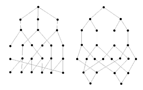
Figure 1: The graph ${\O}_{3}$ as an example of distance-biregular graph.

In particular, every distance-biregular graph $\Gamma$ is semiregular, that is, all vertices in the same independent set have the same degree. If vertices in $V_{i}$ have degree $\delta_{i}$, $i=1,2$, we say that $\Gamma$ is $(\delta_{1},\delta_{2})$-semiregular. In this case, the normalized positive eigenvector of $\Gamma$ is ${\mbox{\boldmath$\alpha$}}=(\alpha_{1}^{n_{1}},\alpha_{2}^{n_{2}})^{\top}$, where

$$\alpha_{1}=\sqrt{\frac{\delta_{1}+\delta_{2}}{2\delta_{2}}}=\sqrt{\frac{n}{2n_{1}}}\qquad\mbox{and}\qquad\alpha_{2}=\sqrt{\frac{\delta_{1}+\delta_{2}}{2\delta_{1}}}=\sqrt{\frac{n}{2n_{2}}}.$$ (3)

A more general framework for studying distance-biregular graphs, which we use here, is that of pseudo-distance-regularity, a concept introduced by Fiol, Garriga, and Yebra in [14]. A graph $\Gamma$ is said to be pseudo-distance-regular around a vertex $u\in V$ with eccentricity $\mathop{\rm ecc}\nolimits(u)=\mbox{$\varepsilon_{u}$}$ if the numbers, defined for any vertex $v\in\Gamma_{i}(u)$,

$$c_{i}^{*}(v)=\frac{1}{\alpha_{v}}\sum_{w\in\Gamma_{i-1}(u)\cap\Gamma(v)}\alpha_{w},\quad a_{i}^{*}(v)=\frac{1}{\alpha_{v}}\sum_{w\in\Gamma_{i}(u)\cap\Gamma(v)}\alpha_{w},\quad b_{i}^{*}(v)=\frac{1}{\alpha_{v}}\sum_{w\in\Gamma_{i+1}(u)\cap\Gamma(v)}\alpha_{w},$$

depend only on the value of $i=0,1,\ldots,\mbox{$\varepsilon_{u}$}$. In this case, we denote them by $c_{i}^{*}$, $a_{i}^{*}$, and $b_{i}^{*}$, respectively, and they are referred to as the $u$-local pseudo-intersection numbers of $\Gamma$.

In the main result of this paper we use the following theorems of Fiol and Garriga [12, 13, 10]. The first one can be considered as the spectral excess theorem for pseudo-distance-regular graphs:

Theorem 3.1 ([12, 13]).

Let $u$ be a vertex of a graph $\Gamma$, with $d_{u}+1$ distinct local eigenvalues, and sum of predistance polynomials $q_{j}^{u}=p_{0}^{u}+\cdots+p_{j}^{u}$. Then, for any polynomial $r\in\mathbb{R}_{j}[x]$ with $j\leq d_{u}$,

$$\frac{r(\lambda_{0})}{\|r\|_{i}}\leq\frac{1}{\alpha_{u}}\|{\mbox{\boldmath$\rho$}}_{N_{j}(u)}\|,$$ (4)

and equality holds if and only if $r=\eta q_{j}^{u}$ for any $\eta\in\mathbb{R}$. Moreover, equality holds with $j=d_{u}-1$ if and only $u$ has maximum eccentricity $d_{u}$ and $\Gamma$ is pseudo-distance-regular around $u$.

A graph $\Gamma$ is said to be pseudo-distance-regularized when it is pseudo-distance-regular graph around each of its vertices. Generalizing a result of Godsil and Shawe-Taylor [15], the author proved the following:

Theorem 3.2 ([10]).

Every pseudo-distance-regularized graph $\Gamma$ is either distance-regular or distance-biregular.

The spectral excess theorem for distance-biregular graphs

Now we are ready to prove the main result of the paper.

Theorem 3.3.

Let $\Gamma$ be a bipartite $(\delta_{1},\delta_{2})$-regular on $n_{1}+n_{2}$ vertices, and with $d+1$ distinct eigenvalues. Let $\Gamma$ have average numbers $\overline{k}_{d}$, $\overline{k}_{1,d}$, $\overline{k}_{2,d}$, $\overline{k}_{2,d-1}$, and highest degree polynomials $p_{d}$, $p_{1,d}$, $p_{2,d}$, $p_{2,d-1}^{*}$ defined as above. Then, $\Gamma$ is distance-biregular if and only if some of the following conditions holds:

• $d$ is odd or $n_{1}=n_{2}$, and $\overline{k}_{d}=p_{d}(\lambda_{0})$.

• $d$ is even, $m(0)\neq|n_{1}-n_{2}|$, and $\overline{k}_{1,d}=p_{1,d}(\lambda_{0})$, $\overline{k}_{2,d}=p_{2,d}(\lambda_{0})$.

• $d$ is even, $m(0)=|n_{1}-n_{2}|$, say $m(0)=n_{1}-n_{2}$, and $\overline{k}_{1,d}=p_{1,d}(\lambda_{0})$, $\overline{k}_{2,d-1}=p_{2,d-1}^{*}(\lambda_{0})$.

Proof.

We only take care of the difficult part, which is to prove sufficiency.

$(a)$ If $n_{1}=n_{2}$, then $\Gamma$ is regular and the result is just the spectral excess theorem for distance-regular graphs. If $d$ is odd we are in case $(ii)$ discussed above, and $p_{1,d}$ and $p_{2,d}$ are multiples of the predistance polynomial $p_{d}$. Then, reasoning as in the proof of case $(b)$, see below, we have that $\Gamma$ is distance-biregular if and only if $p_{1,d}(\lambda_{0})=\frac{2n_{1}}{n}p_{d}(\lambda_{0})=\overline{k}_{1,d}$ and $p_{2,d}(\lambda_{0})=\frac{2n_{2}}{n}p_{d}(\lambda_{0})=\overline{k}_{2,d}$. But, as $d$ is odd, by counting in two ways the number of pairs of vertices at distance $d$, we have that $n_{1}\overline{k}_{1,j}=n_{2}\overline{k}_{2,j}$. Then, putting all together, we get that $n_{1}^{2}=n_{2}^{2}$, and $\Gamma$ must be again regular.

To prove $(b)$, we first claim that, with $r=q_{1,d-1}$, the inequality (4) can be written as

$$\frac{\alpha_{u}^{2}q_{1,d-1}(\lambda_{0})^{2}}{\|{\mbox{\boldmath$\rho$}}_{N_{d-1}(u)}\|^{2}}\leq\|q_{1,d-1}\|_{u}^{2}.$$ (5)

Indeed, if $d_{u}=d$ the result is obvious, whereas if $d_{u}<d$, then $q_{d-1}=r\in\mathbb{R}_{d_{u}}[x]$. Here equality must be understood in the quotient ring $\mathbb{R}[x]/I$, where $I$ is the ideal generated by the polynomial with zeros the $d_{u}+1$ eigenvalues having non-null $u$-local multiplicity. Thus, $\|{\mbox{\boldmath$\rho$}}_{N_{j}(u)}\|\leq\|{\mbox{\boldmath$\rho$}}_{N_{d-1}(u)}\|$, where $j=\deg r$, and the inequality in (4) still holds.

Now, by taking the average over all vertices of $V_{1}$, we have

$$\frac{q_{1,d-1}(\lambda_{0})^{2}}{n_{1}}\sum_{u\in V_{1}}\frac{\alpha_{u}^{2}}{\|{\mbox{\boldmath$\rho$}}_{N_{d-1}(u)}\|^{2}}\leq\frac{1}{n_{1}}\sum_{u\in V}\|q_{1,d-1}\|_{u}^{2}=\|q_{1,d-1}\|_{V_{1}}^{2}=q_{1,d-1}(\lambda_{0}),$$

where we used (1). Consequently,

$$q_{1,d-1}(\lambda_{0})\leq\frac{n_{1}}{\sum_{u\in V_{1}}\frac{\alpha_{u}^{2}}{\|{\mbox{\boldmath$\rho$}}_{N_{d-1}(u)}\|^{2}}}=\frac{2n_{1}}{n}h_{d-1},$$ (6)

where we used that, as $d$ is even, $\alpha_{u}^{2}=n/2n_{1}$, and $h_{d-1}$ stands for the harmonic mean of the numbers $\|{\mbox{\boldmath$\rho$}}_{N_{d-1}(u)}\|^{2}=\|{\mbox{\boldmath$\rho$}}_{V}\|^{2}-\|{\mbox{\boldmath$\rho$}}_{\Gamma_{d}(u)}\|^{2}=n-\|{\mbox{\boldmath$\rho$}}_{\Gamma_{d}(u)}\|^{2}$. Furthermore, since the harmonic mean is at most the arithmetic mean,

$$\frac{2n_{1}}{n}h_{d-1}\leq\frac{2n_{1}}{n}\frac{1}{n_{1}}\sum_{u\in V_{1}}(n-\|{\mbox{\boldmath$\rho$}}_{\Gamma_{d}(u)}\|^{2})=\frac{2}{n}\left(nn_{1}-\frac{n}{2n_{1}}\sum_{u\in V_{1}}k_{d}(u)\right)=2n_{1}-\overline{k}_{1,d}.$$

This, together with $q_{1,d-1}(\lambda_{0})=q_{1,d}(\lambda_{0})-p_{1,d}(\lambda_{0})=2n_{1}-p_{1,d}(\lambda_{0})$ (recall that in the scalar product $\langle\cdot,\cdot\rangle_{V_{1}}$ we have $w_{0}=1/2n_{1}$), gives

$$p_{1,d}(\lambda_{0})\geq\overline{k}_{1,d}.$$ (7)

Then, in case of equality all inequalities in (5) must be also equalities and, from Theorem 3.1, $\Gamma$ is pseudo-distance-regular around each vertex $u\in V_{1}$. In the same way, we prove that, if $p_{2,d}(\lambda_{0})=\overline{k}_{2,d}$, then $\Gamma$ is pseudo-distance-regular around each vertex $v\in V_{2}$. Consequently, $\Gamma$ is a pseudo-distance-regularized graph and, by Theorem 3.2, it is also distance-biregular.

The proof of $(c)$ is analogous and uses the scalar products of case $(iv)$ at the end of Section 2. $\Box$

Observations

We end the paper with some comments.

• Notice that, in cases $(a)$ and $(b)$ the diameters of $\Gamma$ turn to be $D=D_{1}=D_{2}=d$, whereas in case $(c)$ we have $D=D_{1}=d$ and $D_{2}=d-1$. As an example of the latter we have again the subdivided Petersen graph of Fig. 1.

• By using Lemma 2.1$(b)$ we can give explicit formulae for the values of the predistance polynomials at $\lambda_{0}$ appeared in Theorem 3.3. For instance, in case $(c)$,

  $$p_{1,d}(\lambda_{0}) =\textstyle n_{2}\left(\sum_{i=0}^{d/2-1}\frac{\pi_{0}^{2}}{m(\lambda_{i})\pi_{i}^{2}}+\frac{\pi_{0}^{2}}{4m(0)\pi_{d/2}^{2}}\right)^{-1},$$

  $$p_{2,d-1}^{*}(\lambda_{0}) =\textstyle n_{2}\left(\sum_{i=0}^{d/2-1}\frac{\pi_{0}^{2}}{m(\lambda_{i})\pi_{i}^{2}}\right)^{-1}.$$

  where the moment-like parameters $\pi_{i}^{\prime}s$ are defined as before.

• Since the conclusions in $(b)$ and $(c)$ are derived from two inequalities, we can add up the corresponding equalities to give only one condition, as in $(a)$, and the result still holds. For instance, the condition in case (b) can be

  $$\overline{k}_{1,d}+\overline{k}_{2,d}=(p_{1,d}+p_{2,d})(\lambda_{0}).$$

Acknowledgments. Research supported by the Ministerio de Educación y Ciencia (Spain) and the European Regional Development Fund under project MTM2011-28800-C02-01, and by the Catalan Research Council under project 2009SGR1387.

References

- [1] N. Biggs, Algebraic Graph Theory, Cambridge University Press, Cambridge, 1974, second edition, 1993.
- [2] A.E. Brouwer, A.M. Cohen, and A. Neumaier, Distance-Regular Graphs, Springer-Verlag, Berlin-New York, 1989.
- [3] A.E. Brouwer and W.H. Haemers, Spectra of Graphs, Springer, 2012; available online at http://homepages.cwi.nl/~aeb/math/ipm/.
- [4] M. Cámara, J. Fàbrega, M.A. Fiol, and E. Garriga, Some families of orthogonal polynomials of a discrete variable and their applications to graphs and codes, Electron. J. Combin. 16(1) (2009), #R83.
- [5] D. M. Cvetković, M. Doob and H. Sachs, Spectra of Graphs. Theory and Application, VEB Deutscher Verlag der Wissenschaften, Berlin, second edition, 1982.
- [6] C. Dalfó, E.R. van Dam, M.A. Fiol, E. Garriga, and B.L. Gorissen, On almost distance-regular graphs, J. Combin. Theory Ser. A 118 (2011), no. 3, 1094–1113.
- [7] E.R. van Dam, The spectral excess theorem for distance-regular graphs: a global (over)view, Electron. J. Combin. 15(1) (2008), #R129.
- [8] C. Delorme, Distance biregular bipartite graphs, Europ. J. Combin. 15 (1994), 223–238.
- [9] M.A. Fiol, Algebraic characterizations of distance-regular graphs, Discrete Math. 246 (2002), 111–129.
- [10] M.A. Fiol, Pseudo-distance-regularized graphs are distance-regular or distance-biregular, Linear Algebra Appl. 437 (2012), no. 12, 2973–2977.
- [11] M.A. Fiol, S. Gago, and E. Garriga, A simple proof of the spectral excess theorem for distance-regular graphs, Linear Algebra Appl. 432 (2010), no. 9, 2418–2422.
- [12] M.A. Fiol and E. Garriga, From local adjacency polynomials to locally pseudo-distance-regular graphs, J. Combin. Theory Ser. B 71 (1997), 162–183.
- [13] M.A. Fiol and E. Garriga, On the algebraic theory of pseudo-distance-regularity around a set, Linear Algebra Appl. 298 (1999), 115–141.
- [14] M.A. Fiol, E. Garriga and J.L.A. Yebra, Locally pseudo-distance-regular graphs, J. Combin. Theory Ser. B 68 (1996), no. 2, 179–205.
- [15] C.D. Godsil and J. Shawe-Taylor, Distance-regularised graphs are distance-regular or distance-biregular, J. Combin. Theory Ser. B 43 (1987) 14–24.
- [16] A.J. Hoffman, On the polynomial of a graph, Amer. Math. Monthly 70 (1963) 30–36.