Bayesian Inference for Logistic Regression Models using Sequential Posterior Simulation

Abstract

The logistic specification has been used extensively in non-Bayesian statistics to model the dependence of discrete outcomes on the values of specified covariates. Because the likelihood function is globally weakly concave estimation by maximum likelihood is generally straightforward even in commonly arising applications with scores or hundreds of parameters. In contrast Bayesian inference has proven awkward, requiring normal approximations to the likelihood or specialized adaptations of existing Markov chain Monte Carlo and data augmentation methods. This paper approaches Bayesian inference in logistic models using recently developed generic sequential posterior simulaton (SPS) methods that require little more than the ability to evaluate the likelihood function. Compared with existing alternatives SPS is much simpler, and provides numerical standard errors and accurate approximations of marginal likelihoods as by-products. The SPS algorithm for Bayesian inference is amenable to massively parallel implementation, and when implemented using graphical processing units it is more efficient than existing alternatives. The paper demonstrates these points by means of several examples.

1 Introduction

The multinomial logistic regression model, hereafter “logit model,” is one of the most widely used models in applied statistics. It provides one of the simplest and most straightforward links between the probabilities of discrete outcomes and covariates. More generally, it provides a workable probability distribution for discrete events, whether directly observed or not, as a function of covariates. In the latter, more general, setting it is a key component of conditional mixture models including the mixture of experts models introduced by Jacobs et al. (1991) and studied by Jiang and Tanner (1999).

The logit model likelihood function is unimodal and globally concave, and consequently estimation by maximum likelihood is practical and reliable even in models with many outcomes and many covariates. However, it has proven less tractable in a Bayesian context, where effective posterior simulation has been a challenge. Because it also arises frequently in more complex contexts like mixture models, this is a significant impediment to the penetration of posterior simulation methods. Indeed, the multinomial probit model has proven more amenable to posterior simulation methods (Albert and Chib, 1993; Geweke et al., 1994) and has sometimes been used in lieu of the logit model in conditional mixture models (Geweke and Keane, 2007). Thus there is a need for simple and reliable posterior simulation methods for logit models.

State-of-the-art approaches to posterior simulation for logit models use combinations of likelihood function approximation and data augmentation in the context of Markov chain Monte Carlo (MCMC) algorithms: see Holmes and Held (2006), Frühwirth and Frühwirth-Schnatter (2007), Scott (2011), Gramacy and Polson (2012) and Polson et al. (2012). The last paper uses a novel representation of latent variables based on Polya-Gamma distributions that can be applied in logit and related models, and uses this representation to develop posterior simulators that are reliable and substantially dominate alternatives with respect to computational efficiency. Going forward, we refer to the method of Polson et al. (2012) as the PSW algorithm.

This paper implements a sequential posterior simulator (SPS) using ideas developed in Durham and Geweke (2012). Unlike MCMC this algorithm is especially well-suited to massively parallel computation using graphical processing units (GPUs). The algorithm is highly generic; that is, the coding effort required to adapt it to a specific model is typically minimal. In particular, the algorithm is far simpler to implement for the logit models considered here than the existing MCMC algorithms mentioned in the previous paragraph. When implemented on GPUs the computational efficiency of SPS compares favorably with existing MCMC methods, but even on ubiquitous quadcore machines it is still competitive, if slower. Moreover, SPS yields an accurate approximation of log marginal likelihood, as well as reliable and systematic indications of the accuracy of posterior moment approximations, which existing MCMC methods do not.

Section 2 of the paper describes the SPS algorithm and its implementation on GPUs, with emphasis on the specifics of the logit model. Section 3 provides the background for the examples taken up subsequently: specifics of the models and prior distributions, the data sets, and the various hardware and software environments used. Section 4 documents some of the features of models and data sets that govern computation time using SPS. Section 5 studies several applications of the logit model using data sets typical of applied work in biostatistics and the social sciences. Section 6 concludes with some more general observations. A quick first reading of the paper might skim Section 2 and skip Section 4.

2 Sequential Monte Carlo algorithms for Bayesian inference

Sequential posterior simulation (SPS) grows out of sequential Monte Carlo (SMC) methods developed over the past twenty years for state space models, in particular particle filters. Contributions leading up to the development here include Baker (1985, 1987), Gordon et al. (1993), Kong et al. (1994), Liu and Chen (1995, 1998), Chopin (2002, 2004), Del Moral et al. (2006), Andreiu et al. (2010), Chopin and Jacob (2010), and Del Moral et al. (2011). Despite its name, SPS is amenable to massively parallel implementation. It is nearly ideally suited to graphical processing units, which provide massively parallel desktop computing at a cost of well under one dollar (US) per processing core. For further background on these details see Durham and Geweke (2012).

2.1 Conditions

The multinomial logit model assigns probabilities to random variables $Y_{t}\in\left\{1,2,\ldots,C\right\}$ as functions of observed covariates $x_{t}$ and a parameter vector $\theta$. In the simplest setup $\theta^{\prime}=\left(\theta_{1}^{\prime},\ldots,\theta_{C}^{\prime}\right)$ and

$$P\left(Y_{t}=c\mid x_{t},\theta\right)=\frac{\exp\left(\theta_{c}^{\prime}x_{t}\right)}{\sum_{i=1}^{C}\exp\left(\theta_{i}^{\prime}x_{t}\right)}\text{ }\left(c=1,\ldots,C;t=1,\ldots,T\right)\text{.}$$ (1)

There is typically a normalization $\theta_{c}=0$ for some $c\in\left\{1,2,\ldots,C\right\}$, and there could be further restrictions on $\theta$, but these details are not important to the main points of this section. For the properties of the SPS algorithm discussed subsequently what matters is that the likelihood function implied by (1) is (a) bounded and (b) easy to evaluate to machine accuracy. The SPS algorithm also requires (c) a proper prior distribution from which one can simulate $\theta$. We will confine ourselves to the approximation of posterior moments of the form

$$\overline{g}=\mathrm{E}\left[g\left(\theta\right)\mid y_{1:T},x_{1:T}\right]$$

for which (d) $\mathrm{E}\left[g\left(\theta\right)^{2+\delta}\right]$ (some $\delta>0$) exists under the prior distribution. For example, if the prior distribution is Gaussian then condition (c) is satisfied and if the function of interest is a log odds-ratio evaluated at a particular value of the covariate vector, then condition (d) is also met.

For many posterior simulation algorithms yielding a sequence $\left\{\theta_{n}\right\}$, it is known that under these conditions the mean from a sample of size $N$ from the simulator, $\overline{g}^{N}=N^{-1}\sum_{n=1}^{N}g\left(\theta_{n}\right)$, satisfies a central limit theorem

$$N^{1/2}\left(\overline{g}^{N}-\overline{g}\right)\overset{d}{\longrightarrow}N\left(0,v\right)\text{.}$$ (2)

For example, this is the case in many, arguably most, implementations of the Metropolis-Hastings random walk algorithm. It is also true for the SPS algorithm detailed in the next section.

Prudent use of posterior simulation requires that it be possible to compute a simulation-consistent approximation of $v$ in (2), $v^{N}\overset{a.s.}{\longrightarrow}v$. This has proved difficult in the case of MCMC (Flegal and Jones, 2010) and it appears the problem has been ignored in the SMC literature. But, as suggested by Durham and Geweke (2012), one can always work around this difficulty by undertaking $J$ independent replications of the algorithm. Given posterior draws $g_{jn}=g\left(\theta_{jn}\right)$ $\left(j=1,\ldots,J;\text{ }n=1,\ldots,N\right)$, group means are given by

$$\overline{g}_{j}^{N}=N^{-1}\sum_{n=1}^{N}g_{jn}\text{ \ }\left(j=1,\ldots,J\right)\text{;}$$ (3)

and from (2) satisfy

$$N^{1/2}\left(\overline{g}_{j}^{N}-\overline{g}\right)\overset{d}{\longrightarrow}N\left(0,v\right)\text{ \ }\left(j=1,\ldots,J\right)\text{.}$$ (4)

For approximation of the posterior moment we can then use the grand mean

$$\overline{g}^{\left(J,N\right)}=J^{-1}\sum_{j=1}^{J}\overline{g}_{j}^{N}\text{,}$$ (5)

which suggests using the natural approximation of $v$ in (4),

$$\widehat{v}^{\left(J,N\right)}\left(g\right)=\left[N/\left(J-1\right)\right]\sum_{j=1}^{J}\left(\overline{g}_{j}^{N}-\overline{g}^{\left(J,N\right)}\right)^{2}\text{}$$ (6)

to approximate $v$ in (2).

We will define the numerical standard error of $\overline{g}^{\left(J,N\right)}$

$$\mathrm{NSE}\left(\overline{g}^{\left(J,N\right)}\right)=\left[J^{-1}\widehat{v}^{\left(J,N\right)}\left(g\right)\right]^{1/2}\text{.}$$ (7)

As $N\rightarrow\infty$

$$\left(J-1\right)\widehat{v}^{\left(J,N\right)}\left(g\right)/v\overset{d}{\rightarrow}\chi^{2}\left(J-1\right)\text{}$$ (8)

and

$$\frac{\overline{g}^{\left(J,N\right)}-\overline{g}}{\mathrm{NSE}\left(\overline{g}^{\left(J,N\right)}\right)}\overset{d}{\rightarrow}t\left(J-1\right)\text{.}$$ (9)

The NSE provides a measure of the variability of the moment approximation (5) across replications of the algorithm with fixed data.

The relative numerical efficiency (RNE; Geweke 1989), which approximates the population moment ratio $\mathrm{var}\left(g\left(\theta\right)\mid y_{1:T}\right)/v$, can be obtained in a similar manner,

$$\mathrm{RNE}\left(\overline{g}^{\left(J,N\right)}\right)=\left(JN\right)^{-1}\sum_{j=1}^{J}\sum_{n=1}^{N}\left(g_{jn}-\overline{g}^{\left(J,N\right)}\right)^{2}/\widehat{v}^{\left(J,N\right)}\left(g\right)\text{.}$$ (10)

RNE close to one indicates that there is little dependence amongst the particles, and that the moment approximations (3) and (5) approach the efficiency of the ideal, an iid sample from the posterior. RNE less than one indicates dependency. In this case, the moment approximations (3) and (5) are less precise than one would obtain with a hypothetical iid sample.

This is all rather awkward for MCMC, requiring as it does $J$ repetitions of the algorithm complete with burn-in; we use it in Sections 3 and 4 to assess the accuracy of posterior moment approximations of the Polson et al. (2012) procedure, in the absence of a better alternative. However, the procedure is natural in the context of the SPS algorithm, requires no additional computations, and makes efficient use of massively parallel computing environments (Durham and Geweke, 2012).

Going forward in this section, $p\left(\theta\right)$ denotes the prior density of $\theta$. The vectors $y_{1},\ldots,y_{T}$ denote the data and $y_{1:t}=\left\{y_{1},\ldots,y_{t}\right\}$. The notation suppresses conditioning on the covariates $x_{t}$ and treats all distributions as continuous to avoid notational clutter. Thus, for example, the likelihood function is

$$p\left(y_{1:T}\mid\theta\right)=\prod\limits_{t=1}^{T}p\left(y_{t}\mid y_{1:t-1},\theta\right)\text{.}$$

2.2 Non-adaptive SPS algorithms

We begin with a mild generalization of the SMC algorithm of Chopin (2004). The algorithm generates and modifies different values of the parameter vector $\theta$, known as particles and denoted $\theta_{jn}$, with superscripts used for further specificity at various points in the algorithm. The subscripts refer to the $J$ groups of $N$ values each described in the previous section. To make the notation compact, let $\mathcal{J}\!=\left\{1,\ldots,J\right\}\,\$and $\mathcal{N=}\left\{1,\ldots,N\right\}$. The algorithm is an implementation of Bayesian learning, providing simulations from $\theta\mid y_{1:t}$ for $t=1,2,\ldots,T$. It processes observations, in order and in successive batches, each batch constituting a cycle of the algorithm.

The global structure of the algorithm is therefore iterative, proceeding through the sample. But it operates on many particles in exactly the same way at almost every stage, and it is this feature of the algorithm that makes it amenable to massively parallel implementations. On conventional quadcore machines and samples of typical size one might set up the algorithm with $J=10$ groups of $1000$ particles each, and using GPUs $J=40$ groups of $2500$ particles each. (The numbers are just illustrations, to fix ideas.)

Algorithm 1

(Nonadaptive)  Let $t_{0},\ldots,t_{L}$ be fixed integers with $0=t_{0}<t_{1}<\ldots<t_{L}=T$; these define the cycles of the algorithm. Let $\lambda_{1},\ldots,\lambda_{L}$ be fixed vectors that parameterize transition distributions as indicated below.

1. Initialize $\ell=0$ and let $\theta_{jn}^{\left(\ell\right)}\overset{iid}{\thicksim}p\left(\theta\right)\quad\left(j\in\mathcal{J}\!,\,n\in\mathcal{N}\right)$

2. For $\ell=1,\dots,L$

   1. Correction $\left(C\right)$ phase, for all $j\in\mathcal{J}$ and $\,n\in\mathcal{N}$:

      1. $w_{jn}\left(t_{\ell-1}\right)=1$

      2. For $s=t_{\ell-1}+1,\dots,t_{\ell}$

         $$w_{jn}\left(s\right)=w_{jn}\left(s-1\right)\cdot p\left(y_{s}\mid y_{1:s-1},\theta_{jn}^{\left(\ell-1\right)}\right)$$ (11)

      3. $w_{jn}^{\left(\ell-1\right)}:=w_{jn}\left(t_{\ell}\right)$

   2. Selection $\left(S\right)$ phase, applied independently to each group $j\in\mathcal{J}$: Using multinomial or residual sampling based on $\left\{w_{jn}^{\left(\ell-1\right)}\,\left(n\in\mathcal{N}\right)\right\}$, select

      $$\left\{\theta_{jn}^{\left(\ell,0\right)}\,\left(n\in\mathcal{N}\right)\right\}\text{ from }\left\{\theta_{jn}^{\left(\ell-1\right)}\,\left(n\in\mathcal{N}\right)\right\}$$

   3. Mutation $\left(M\right)$ phase, applied independently across $j\in\mathcal{J}\!,\,n\in\mathcal{N}$:

      $$\theta_{jn}^{\left(\ell\right)}\thicksim p\left(\theta\mid y_{1:t_{\ell}},\theta_{jn}^{\left(\ell,0\right)},\lambda_{\ell}\right)\text{}$$ (12)

      where the drawings are independent and the p.d.f. (12) satisfies the invariance condition

      $$\int_{\Theta}p\left(\theta\mid y_{1:t_{\ell}},\theta^{\ast},\lambda_{\ell}\right)p\left(\theta^{\ast}\mid y_{1:t_{\ell}}\right)d\nu(\theta^{\ast})=p\left(\theta\mid y_{1:t_{\ell}}\right)$$ (13)

3. $\theta_{jn}:=\theta_{jn}^{\left(L\right)}\quad\left(j\in\mathcal{J}\!,\,n\in\mathcal{N}\right)$

The algorithm is nonadaptive because $t_{0},\ldots,t_{L}$ and $\lambda_{1},\ldots,\lambda_{L}$ are fixed before the algorithm starts. Going forward it will be convenient to denote the cycle indices by $\mathcal{L}=\left\{1,\ldots,L\right\}$. At the conclusion of the algorithm, the simulation approximation of a generic posterior moment is (5).

The only communication between particles is in the $S$ phase. In the $C$ and $M$ phases exactly the same computations are made for each particle, with no communication. This situation is ideal for GPUs, as detailed in Durham and Geweke (2012). In the $S$ phase there is communication between particles within, but not across, the $J$ groups. This keeps the particles in the $J$ groups independent. Typically the fraction of computation time devoted to the $S$ phase is minute.

For each group, $j\in\mathcal{J}\!$, the four regularity conditions in the previous section imply the assumptions of Chopin (2004), Theorem 1 (for multinomial resampling) and Theorem 2 (for residual resampling). Therefore a central limit theorem (2) applies. Chopin provides population expressions for $v$ in terms of various unknown moments but neither that paper, nor to our knowledge any other paper, provides a way to approximate $v$.

The approach described in the previous section solves this problem.  Notice that dependence amongst the particles arises solely from the $S$ phase, in which resampling is applied independently to each group $j\in\mathcal{J}$: Therefore the $J$ partial means $\overline{g}_{j}^{N}$ are mutually independent for all $N$. The procedures for approximating $v$, numerical standard errors, and a large-$N$ theory of numerical accuracy laid out in (3) - (9) therefore apply.

2.3 Adaptive SPS algorithms

In Algorithm 1 neither the cycles, defined by $t_{1},\ldots,t_{L-1}$, nor the hyperparameters $\lambda_{\ell}$ of the transition processes (12) depend on the particles $\left\{\theta_{jn}\right\}$. With respect to the random processes that generate these particles, these hyperparameters are fixed: in econometric terminology, they are predetermined with respect to $\left\{\theta_{jn}\right\}$. As a practical matter, however, one must use the knowledge of the posterior distribution inherent in the particles to choose the transition from the $C$ phase to the $S$ phase, and to design an effective transition distribution in the $M$ phase. Without this feedback it is impossible to obtain an approximation $\overline{g}^{\left(J,N\right)}$ of $\overline{g}$ with acceptably small NSE; indeed, in all but the simplest models and smallest data sets $\overline{g}^{\left(J,N\right)}$ will otherwise be pure noise, for all intents and purposes.

The following procedure illustrates how the particles themselves can be used to choose the cycles defined by $t_{1},\ldots,t_{L-1}$ and the hyperparameters $\lambda_{\ell}$ of the transition processes. It is a minor modification of a procedure first described in Durham and Geweke (2012), that has proved effective in a number of models. It is also effective in the logit model. The algorithm requires that the user choose the number of groups, $J$, and the number of particles in each group, $N$.

Algorithm 2

(Adaptive)

1. Determine the value of $t_{\ell}$ in the $C$ phase of cycle $\ell\,\left(\ell\in\mathcal{L}\right)$ as follows.

   1. At each step $s$ compute the effective sample size

      $$\mathit{ESS}\left(s\right)=\frac{\left[\sum_{j=1}^{J}\sum_{n=1}^{N}w_{jn}\left(s\right)\right]^{2}}{\sum_{j=1}^{J}\sum_{n=1}^{N}w_{jn}\left(s\right)^{2}}\text{}$$ (14)

      immediately after computing (11).

   2. If $\mathit{ESS}\left(s\right)/\left(J\cdot N\right)<0.5$ or if $s=T$ set $t_{\ell}=s$ and proceed to the $S$ phase. Otherwise increment $s$ and recompute (14).

2. The transition density (12) in the $M$ phase of each cycle $\ell$ is a Metropolis Gaussian random walk, executed in steps $r=1,2,\ldots$ .

   1. Initializiations:

      1. $r=1$.

      2. If $\ell=1$ then the step size scaling factor $h_{11}=0.5$.

   2. Set $\mathrm{RNE}$ termination criteria:

      1. If $s<T$, $K=0.35$

      2. If $s=T$, $K=0.9$

   3. Execute the next Metropolis Gaussian random walk step.

      1. Compute the sample variance $V_{\ell r}$ of the particles

         $$\theta_{jn}^{\left(\ell,r-1\right)}\,\,\left(j=1,\ldots,J;n=1,\ldots,N\right),$$

         define $\Sigma_{\ell r}=h_{\ell r}\cdot\,V_{\ell r}$, and execute step $r$ using a random walk Gaussian proposal density with variance matrix $\Sigma_{\ell r}$ to produce a new collection of particles $\theta_{jn}^{\left(\ell,r\right)}\,\left(j=1,\ldots,J;\text{ }n=1,\ldots,N\right)$. Let $\alpha_{\ell r}$ denote the Metropolis acceptance rate across all particles in this step.

      2. Set $h_{\ell,r+1}=\min\left(h_{\ell r}+0.01,1.0\right)$ if $a_{\ell r}>0.25$ and $h_{\ell,r+1}=\max\left(h_{\ell r}-0.01,0.1\right)$ otherwise.

      3. Compute the RNE of the numerical approximation $\overline{g}^{\left(J,N\right)}$ to a test function $g^{\ast}\left(\theta\right)$. If $\mathrm{RNE}<K$ then increment $r$ and return to step 2c; otherwise set $h_{\ell+1,1}=h_{\ell,r+1}$, define $R_{\ell}=r$, and return to step 1.

   4. Set $\theta_{jn}^{(\ell)}=\theta_{jn}^{(\ell,r)}$. If $s<T$  then set $h_{\ell+1,1}=h_{\ell,r+1}$ and return to step 1; otherwise set $\theta_{jn}=\theta_{jn}^{(\ell)}$, define $L=\ell$, and terminate.

At each step of the algorithm particles are identically but not independently distributed. As the number of particles in each group $N\rightarrow\infty$ the common distribution coincides with the posterior distribution. As the number of Metropolis steps, $r$, in the $M$ phase increases, dependence amongst particles decreases. The $M$ phase terminates when the RNE criterion is satisfied, implying a specified degree of independence for the particles at the end of each cycle. Larger values of $J$ provide better estimates of RNE, making this assessment more reliable. The RNE criterion $K$ assures a specified degree of independence at the end of each cycle. The assessment of numerical accuracy is based on the comparison of different approximations in $J$ groups of particles, and larger values of $J$ make this assessment more reliable.

At the conclusion of the algorithm, the posterior moments of interest $E(g(\theta)|y_{1:T})$ are approximated,

$$\overline{g}^{\left(J,N\right)}=\left(JN\right)^{-1}\sum_{j=1}^{J}\sum_{n=1}^{N}g\left(\theta_{jn}\right)\text{.}$$

The asymptotic (in $N$) variance of the approximation is proportional to $\left(JN\right)^{-1}$, and because $K=0.9$ in the last cycle $L$ the factor of proportionality is approximately the posterior variance $\mathrm{var}\left(g\left(\theta\right)\mid y_{1:T}\right)$. As detailed in Section 2.1, the accuracy of the reported NSE is proportional to $J^{-1/2}$.

The division of a given posterior sample size into a number of groups $J$ and particles within groups $N$ should be guided by the tradeoff implied by (8) and the fact that values of $N$ sufficiently small will give misleading representations of the posterior distribution. From (8) notice that the ratio of squared $NSE$ from one simulation to another has an asymptotic (in $N$) $F\left(J-1,J-1\right)$ distribution. For $J=8$, the ratio of $NSE$ in two simulations will be less than 2 with probability 0.95. A good benchmark for serviceable approximation of posterior moments is $J=10$, $N=1000$. With implementation on GPUs much larger values can be practical: Durham and Geweke (2012) use $J=64$ and $N=4096$ in an application that is computationally much more demanding than the examples in this paper.

The statement of Algorithm 2 shows that it contains several algorithm design parameters that are simply fixed. These fixed parameters have been set to ensure that as the algorithm proceeds through the sample it maintains a workable accuracy of approximation, and does so in a computationally efficient manner.

Upon entering the $S$ phase, the effective sample size is less than half the number of particles (except perhaps in the final cycle). After resampling, the number of unique particles is roughly equal to the effective sample size before resampling, but the ESS measure (14) is no longer valid when applied to the new sample (since it does not account for dependence between particles). In the $M$ phase, iterating the Metropolis step reduces dependence between particles, and the RNE after each step provides a way of assessing the effectiveness of the mixing that takes place. When RNE gets close to one, further Metropolis steps are of little utility and a waste of computing resources. Prior to the final cycle we have found it practical to terminate the $M$ phase when RNE exceeds 0.35. In the final cycle, we have found it useful to undertake additional $M$ steps in order to get higher RNE (and lower NSE) when approximating the posterior moments of interest. We suggest a criterion of $\text{RNE}>0.9$ for the final cycle. Since these extra iterations occur only in the final step, the relative cost is low — indeed the cost is typically much lower than the alternative of increasing the number of particles.

Performance of the algorithm is not very sensitive to changes in the ESS criterion. Higher thresholds lead to more cycles but fewer iterations in the $M$ phase; lower values lead to fewer cycles but more time in the $M$ phase. On the other hand, changing the RNE criteria has the effects one might expect. Changing the RNE criterion in the final cycle affects the accuracy of the posterior moment approximations. Changing the RNE criterion for the other cycles does not affect accuracy of posterior moment approximations undertaken at time $T$, but does affect the accuracy of the approximations of log marginal likelihood and log predictive likelihoods. As detailed in Durham and Geweke (2012) , Section 4, these approximations are based on the particle representation of the intermediate posterior distributions $p\left(\theta\mid y_{1:t}\right)$. Increasing 0.35 – say, to 0.9 – will increase the accuracy of the approximation. The effect is to reduce NSE for log marginal likelihood by a factor of roughly $1-\left(0.35/0.9\right)^{1/2}\approxeq 1/3$, and total computing time can increase by 50% or more. We have found the constants suggested above to provide a good balance in the various tradeoffs involved. But the software that supports the work in this paper makes it convenient for the knowledgeable user to change any of the “hardwired” design parameters in Algorithm 2 if desired.

2.4 The two-pass SPS algorithm

Algorithm 2 is practical and reliable in a very wide array of applications. This includes situations in which MCMC is utterly ineffective, as illustrated in Durham and Geweke (2012) and Herbst and Schorfheide (2012). However there is an important drawback: the algorithm has no supporting central limit theorem.

The effectiveness of the algorithm is due in no small part to the fact that the cycle definitions $\left\{t_{\ell}\right\}$ and parameters $\lambda_{\ell}$ of the $M$ phase transition distributions are based on the particles themselves. This creates a structure of dependence amongst particles that is extremely complicated. The degree of complication stemming from the use of effective sample size in step 1b can be managed: see Del Moral et al. (2012). But the degree of complication introduced in the $M$ phase, step 2c, is orders of magnitude larger. This is not addressed by any of the relevant literature, and (in our view) this problem is not likely to be resolved by attacking it directly anytime in the foreseeable future.

Fortunately, the problem can be solved at the cost of roughly doubling the computational burden in the following manner as proposed by Durham and Geweke (2012).

Algorithm 3

(Two pass)

1. Execute the adaptive Algorithm 2. Discard the particles $\left\{\theta_{jn}\right\}$. Retain the number of cycles $L$, values $t_{0},\ldots,t_{L}$ that define the cycles, the number of iterations $R_{\ell}$ executed in each $M$ phase, and the variance matrices $\lambda_{\ell}=\left\{\Sigma_{\ell r}\right\}$ from each $M$ phase.

2. Execute algorithm 2 using $t_{\ell}$, $R_{\ell}$ and $\lambda_{\ell}$ $\left(\ell=1,\ldots,L\right)$.

Notice that in step 2 the cycle break points $t_{0},\ldots,t_{L}$ and the variance matrices $\Sigma_{\ell r}$ are predetermined with respect to the particles generated in that step. Because they are fixed with respect to the process of random particle generation, step 2 is a specific version of Algorithm 1. The only change is in the notation: $\lambda_{\ell}$ in Algorithm 1 is the sequence of matrices $\left\{\Sigma_{\ell r}\right\}$ indexed by $r$ in step 2 of Algorithm 3. The results in Chopin (2004), and other results for SMC algorithms with fixed design parameters, now apply directly.

The software used for the work in this paper makes it convenient to execute the two-pass algorithm. In a variety of models and applications results using Algorithms 2 and 3 have always been similar, as illustrated in Section 4.1. Thus it is not necessary to use the two-pass algorithm exclusively, and we do not recommend doing so in the course of a research project. It is prudent when SPS is first applied to a new model, because there is no central limit theorem for the one-pass algorithm (Algorithm 2), and one should check early for the possibility that this algorithm might be inadequate. Given that Algorithm 3 is available in generic SPS software, and the modest computational cost involved, it is also probably a wise step in the final stage of research before public presentation of findings.

3 Models, data and software

The balance of this paper studies the performance of the SPS algorithm in a variety of situations typical of those in applied work. This section provides full detail of the models used, in Section 3.1, and describes the data sets used in Section 3.2. The paper compares the performance of SPS in a variety of software and hardware environments, and with the state-of-the-art MCMC algorithm described in Polson et al. (2012). Section 3.3 provides the details of the hardware and software used subsequently in Sections 4 and 5 to document the performance of the PSW and SPS algorithms.

3.1 Models

We use the specification (1) of the multinomial logit model throughout. The binomial logit model is the special case $C=2$.  Going forward, denote the covariates $X=\left[x_{1},\ldots,x_{T}\right]^{\prime}$. The log odds-ratio

$$\log\left[\frac{P\left(Y_{t}=i\mid x_{t},\theta\right)}{P\left(Y_{t}=j\mid x_{t},\theta\right)}\right]=\left(\theta_{i}-\theta_{j}\right)^{\prime}x_{t}\text{}$$ (15)

is linear in the parameter vector $\theta$.

While normalization of the parameters is desirable, it is useful to begin with a Gaussian prior distribution with independent components

$$\theta_{c}\overset{iid}{\thicksim}N\left(\mu_{c},\Sigma_{c}\right)\text{ }\left(c=1,\ldots,C\right)\text{.}$$ (16)

This prior distribution implies that the vectors $\theta_{j}-\theta_{c}$ $\left(j=1,\ldots,C;j\not=c\right)$ are jointly normally distributed, with

$$\mathrm{E}\left(\theta_{j}-\theta_{c}\right)=\mu_{j}-\mu_{c}\text{, }\mathrm{var}\left(\theta_{j}-\theta_{c}\right)=\Sigma_{j}+\Sigma_{c}\text{, }\mathrm{cov}\left(\theta_{j}-\theta_{c},\theta_{i}-\theta_{c}\right)=\Sigma_{c}\text{.}$$ (17)

This provides the prior distribution of the parameter vector when (1) is normalized by setting $\theta_{c}=0$, that is, when $\theta_{j}$ is replaced by $\theta_{j}-\theta_{c}$ and $\theta_{c}$ is omitted from the parameter vector. So long as the constancy of the prior distribution (17) is respected, all posterior moments of the form $\mathrm{E}\left[h\left(Y\right)\mid x\right]$ will be invariant with respect to normalization. While it is entirely practical to simulate from the posterior distribution of the unnormalized model, for computation it is more efficient to use the normalized model because the parameter vector is shorter, reducing both computing time and storage requirements.

If the prior distribution (16) is exchangeable across $c=1,\ldots,C$ then there is no further loss of generality in specifying $\mu_{c}=0$ and $\Sigma_{c}=\Sigma$ $\left(c=1,\ldots,C\right)$. In the case studies in Section 5, with one minor exception we restrict $\Sigma$ to the class proposed by Zellner (1986),

$$\Sigma=g\cdot T\cdot\left(X^{\prime}X\right)^{-1}\text{.}$$ (18)

To interpret $\Sigma$, consider the conceptual experiment in which the prior distribution of $\theta$ is augmented with $x_{t}$ drawn with probability $T^{-1}$ from the set $\left\{x_{1},\ldots,x_{T}\right\}$ and then $Y$ is generated by (1). Then the prior distribution of the log odds-ratio (15) is also Gaussian, with variance matrix

$$\frac{1}{T}\sum_{t=1}^{T}x_{t}^{\prime}\left[2gT\left(X^{\prime}X\right)^{-1}\right]x_{t}=\frac{1}{T}\mathrm{tr}\sum_{t=1}^{T}x_{t}x_{t}^{\prime}\left[2gT\left(X^{\prime}X\right)^{-1}\right]=2g\text{.}$$

The log-odds ratio is centered at 0, with a standard deviation of $\left(2g\right)^{1/2}$. Some corresponding 95% credible sets for the log-odds ratio are $\left(\log\left(1/16\right),\log\left(16\right)\right)$ for $g=1$, $\left(\log\left(1/4\right),\log\left(4\right)\right)$ for $g=1/4$, and $\left(\log\left(1/2\right)\log\left(2\right)\right)$ for $g=1/16$.

This provides the substantive interpretation of the prior distribution essential to subjective Bayesian inference.

3.2 Data

We used eight different data sets to study and compare the performance of the PSW and SPS algorithms.  Table 1 summarizes some properties of these data. The notation in the column headings is taken from Section 3.1. from which the number of parameters is $k\cdot\left(C-1\right)$. The values of $g$ in the last column are based on marginal likelihood approximations, discussed further in Section 5.1.

Table 1: Characteristics of data sets

Data set	Sample size $T$	Covariates $k$	Outcomes $C$	Parameters	Modal $g$
Diabetes	768	13	2	13	1/4
Heart	270	19	2	19	1/4
Australia	690	35	2	35	1/4
Germany	1000	42	2	42	1/16
Cars	263	4	3	8	1/4
Caesarean 1	251	8	3	16	1/4
Caesarean 2	251	4	3	8	1
Transportation	210	9	4	27	1

For the binomial logit models, we use the same four data sets as Polson et al. (2012), Section 3.3. Data and documentation may be found at the University of California - Irvine Machine Learning Repository, using the links indicated.

• Data set 1, “Diabetes.” The outcome variable is indication for diabetes using World Health Organization criteria, from a sample of individuals of Pima Indian heritage living near Phoenix, Arizona, USA. Of the covariates, one is a constant and one is a binary indicator. Link: Pima Indians Diabetes

• Data set 2, “Heart.” The outcome is presence of heart disease. Of the covariates, one is a constant and 12 are binary indicators. $T=270$. Link: Statlog (Heart)

• Data set 3, “Australia.” The outcome is approval or denial of an application for a credit card. Of the covariates, one is a constant and 28 are binary indicators. Link: Statlog (Australian Credit Approval)

• Data set 4, “Germany.” The outcome is approval or denial of credit. Of the covariates, one is a constant and 42 are binary indicators. $T=1000$. Link: Statlog (German Credit Data)

For the multinomial logit models, we draw from three data sources. The first two have been used in evaluating approaches to posterior simulation and the last is typical of a simple econometric application.

• Data set 5, “Cars.” The outcome variable is the kind of car purchased (family, work or sporty). Of the covariates, one is continuous and the remainder are binary indicators. The data were used in Scott (2011) in the evaluation of latent variable approaches to posterior simulation in logit models, and are taken from the data appendix of Foster et al. (1998).

• Data set 6, “Caesarean 1.” The outcome variable is infection status at birth (none, Type 1, Type 2). The covariates consist of a constant and three binary indicators. These data (Farhmeir and Tutz, 2001, Table 1.1) have been a widely used test bed for the performance posterior simulators given severely unbalanced contingency tables, for example Frühwirth-Schnatter and Frühwirth (2012) and references therein. The data are distributed with the $R$ statistical package.

• Data set 7, “Caesarean 2.” The data are the same as in the previous set, except that the model is fully saturated: there are eight covariates, one for each combination of indicators. This variant of the model has been widely studied because the implicit design is severely unbalanced. One cell is empty. For the sole purpose of constructing the $g$ prior (18) we supplement the covariate matrix $X$ with a single row having an indicator in the empty cell. The likelihood function uses the actual data.

• Data set 8, “Transportation.” The data is a choice-based sample of mode of transportation choice (car, bus, train, air) between Sydney and Melbourne. The covariates are all continuous except for the intercept. The data (Table F21.2 of the data appendix of Greene (2003) are widely used to illustrate logit choice models in econometrics.

3.3 Hardware and software

The PSW algorithm is described in Polson et al. (2012). The code is the R package BayesLogit provided by the authors. Except as noted in Section 5.1, the code executed flawlessly without intervention. The execution used a 12-core CPU ($2\times$ Intel Xeon 5680) and 24G memory, but the code does not exploit the multiple cores.

The SPS/CPU algorithm used the algorithm described in Section 2 The code is written in Matlab Edition 2012b (with the Statistics toolbox) and will be made available shortly with the next revision of this paper.  The execution used a 12-core CPU ($2\times$ Intel Xeon E5645) and 24B memory, exploiting multiple cores with a ratio of CPU to wall clock time of about 5. 

The SPS/GPU algorithm used the algorithm described in Section 2. The code is written Matlab Edition 2012a (with the Statistics and Parallel toolboxes) and uses the C extension CUDA version 4.2 and will be made available shortly with the next revision of this paper . The execution used an Intel Core i7 860, 2.8 GHz CPU and one Nvidia GTX 570 GPU (480 cores).

4 Performance of the SPS algorithm

The SPS algorithm can be used routinely in any model that has a bounded and directly computed likelihood function, accompanied by a proper prior distribution. The algorithm performs consistently without intervention from the user. It provides numerical standard errors that are reliable in the sense that they indicate correctly the likely outcome of a repeated, independent execution of the sequential posterior simulator. As a by-product, it also provides consistent (in $N$) approximations of log marginal likelihood and associated numerical standard error; Section 4 of Durham and Geweke (2012) explains the procedure. Section 4.1, below, illustrates these properties for the case of the multinomial logit model. The frequency of transition from one cycle to a new cycle as well as the number of steps taken in the $M$ phase, and therefore the execution time, depend on characteristics of the model and the data. Section 4.2 studies some aspects of this dependence for the case of the multinomial logit model.

4.1 Reliability of the SPS algorithm

Numerical approximations of posterior moments must be accompanied by an indication of their accuracy. Even if editorial constraints make it impossible to accompany each moment approximation with an indication of accuracy, decent scholarship demands that the investigator be aware of the accuracy of reported moment approximations. Moreover, the accuracy indications must themselves be interpretable and reliable.

The SPS methodology for the logit model described in Section 2 achieves this standard by means of a central limit theorem for posterior moment approximations accompanied by a scheme for grouping particles that leads to a simple simulation-consistent approximation of the variance in the central limit theorem. The practical manifestation of these results is the numerical standard error (7). The underlying theory for SPS requires the two-pass procedure of Algorithm 3. If the theory is adequate, then numerical standard errors form the basis for reliable predictions of the outcome of repeated simulations.

Table 2: Reliability of one- and two-pass algorithms

	$\mathrm{E}\left(\theta_{1}^{\prime}\overline{x}\mid\mathrm{Data}\right)$	$\mathrm{E}\left(\theta_{2}^{\prime}\overline{x}\mid\mathrm{Data}\right)$	$\log$ ML
$J=10,N=1000$
Run $A$, Pass 1	0.6869 [.0017]	-0.3836 [.0017]	-253.732 [.057]
Run $A$, Pass 2	0.6855 [.0012]	-0.3856 [.0024]	-253.504 [.086]
Run $B$, Pass 1	0.6811 [.0014]	-0.3920 [.0017]	-253.522 [.082]
Run $B$, Pass 2	0.6847 [.0018]	-0.3877 [.0025]	-253.514 [.054]
Run $C$, Pass 1	0.6844 [.0016]	-0.3892 [.0018]	-253.478 [.055]
Run $C$, Pass 2	0.6837 [.0019]	-0.3875 [.0021]	-253.637 [.065]
$J=40,N=2500$
Run $A$, Pass 1	0.6850 [.00051]	-0.3873 [.00062]	-253.6117 [.026]
Run $A$, Pass 2	0.6857 [.00049]	-0.3871 [.00076]	-253.5934 [.029]
Run $B$, Pass 1	0.6844 [.00043]	-0.3890 [.00061]	-253.6249 [.019]
Run $B$, Pass 2	0.6849 [.00048]	-0.3885 [.00063]	-253.5708 [.027]
Run $C$, Pass 1	0.6853 [.00050]	-0.3881 [.00060]	-253.5918 [.023]
Run $C$, Pass 2	0.6847 [.00043]	-0.3872 [.00052]	-253.5922 [.024]

Table 2 provides some evidence on these points using the multinomial logit model and the cars data set described in Section 3.2. For both small and large SPS executions (upper and lower panels, respectively) Table 2 indicates moment approximations for three independent executions ($A$, $B$ and $C$) of the two-pass algorithm, and for both the first and second pass of the algorithm. The posterior moments used in the illustrations here, and subsequently, are the the log-odds (with respect to the outcome $Y=C$, $\theta_{c}^{\prime}\overline{x}$ $\left(c=1,\ldots,C\right)$, where $\overline{x}$ is the sample mean of the covariates. Numerical standard errors are indicated in brackets. As discussed in Section 2.3, these will vary quite a bit more from one run to another when $J=10$ than they will when $J=40$, and this is evident in Table 2.

Turning first to the comparison of results at the end of Pass 1 (no formal justification for numerical standard errors) and at the end of Pass 2 (the established results for the nonadaptive algorithm discussed in Section 2.2 apply) there are no unusually large differences within any run, given the numerical standard errors. That is, there is no evidence to suggest that if an investigator used Pass 1 results to anticipate what Pass 2 results would be, the investigator would be misled.

This still leaves the question of whether the numerical standard errors from a single run are a reliable indication of what the distribution of Monte Carlo approximations would be across independent runs. Comparing results for runs $A$, $B$ and $C$, Table 2 provides no indication of difficulty for the large SPS executions. For the small SPS executions, there is some suggestion that variation across runs at the end of the first pass is larger than numerical standard error suggests. Note in particular the approximation of log marginal likelihood for runs $A$ and $C$, and note also $E\left(\theta_{1}^{\prime}\overline{x}\right)$ for runs $A$ and $B$.

These suggestions could be investigated more critically with scores or hundreds of runs of the SPS algorithm, but we conjecture the returns would be low and in any event there is no basis for extrapolating results across models and data sets. Most important, one cannot resort to this tactic routinely in applied work. The results here support the earlier recommendation (at the end of Section 2.4) that the investigator proceed mainly using the one-pass algorithm, reserving the two-pass algorithm for checks at the start and the end of a research project.

4.2 Adaptation in the SPS algorithm

The SPS algorithm approximates posterior distributions by mimicking the formal Bayesian updating process, observation by observation, using (at least) thousands of particles simultaneously. It does so in a reliable and robust manner, with much less intervention, problem-specific tailoring, or baby-sitting than is the case with other posterior simulation methods. For example it does not require the investigator to tailor a source distribution for importance sampling (which SPS uses in the $C$ phase) nor does it require that the investigator monitor a Markov chain (which SPS uses in the $M$ phase) for stationarity or serial correlation.

Table 3: Some features of the SMC algorithm for the cars data

	$g=1/64$	$g=1/16$	$g=1/4$	$g=1$	$g=4$
$J=10,N=1000$
Cycles	11	18	24	32	37
M iterations	80	186	189	257	330
Relative time	1.00	2.08	1.47	2.11	2.19
RNE, $\mathrm{E}\left(\theta_{1}^{\prime}\overline{x}\mid\mathrm{Data}\right)$	1.08	1.09	1.02	1.55	1.06
RNE, $\mathrm{E}\left(\theta_{2}^{\prime}\overline{x}\mid\mathrm{Data}\right)$	0.93	0.86	0.83	2.15	2.13
NSE(log ML)	0.088	0.052	0.069	0.075	0.089
$J=40,N=2500$
Cycles	11	18	24	33	37
M iterations	94	131	178	268	319
Relative time	1.00	1.09	1.32	1.76	1.92
RNE, $\mathrm{E}\left(\theta_{1}^{\prime}\overline{x}\mid\mathrm{Data}\right)$	1.00	0.94	1.12	1.17	1.03
RNE, $\mathrm{E}\left(\theta_{2}^{\prime}\overline{x}\mid\mathrm{Data}\right)$	1.12	0.99	1.19	1.23	1.01
NSE(log ML)	0.025	0.027	0.026	0.035	0.037

While SPS requires very little intervention by the user, a little insight into its mechanics helps to understand the computational demands of the algorithm. Table 3 and Figures 1 and 2 break out some details of these mechanics, continuing to use the cars data set from Section 4.1. Figure 1 and the upper panel of Table 3 pertain to the small SPS execution, and Figure 2 and the lower panel of Table 3 pertain to the large SPS execution. They compare performance under all five prior distributions to illustrate some central features of the algorithm.

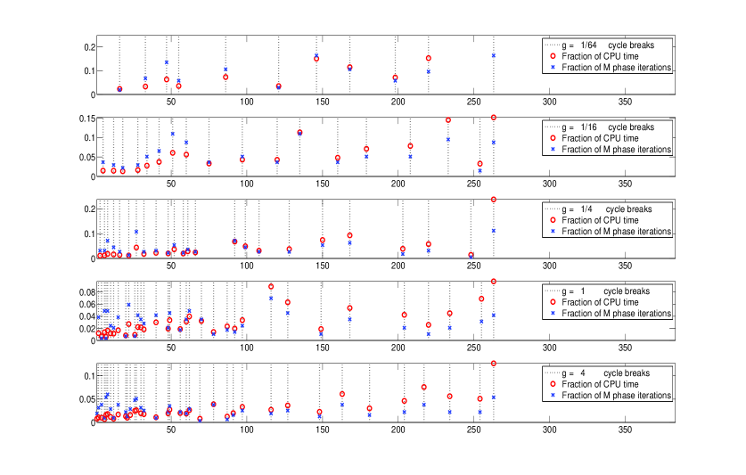
Figure 1: Some properties of the SMC algorithm in the cars example $\left(J=10,N=1000\right)$

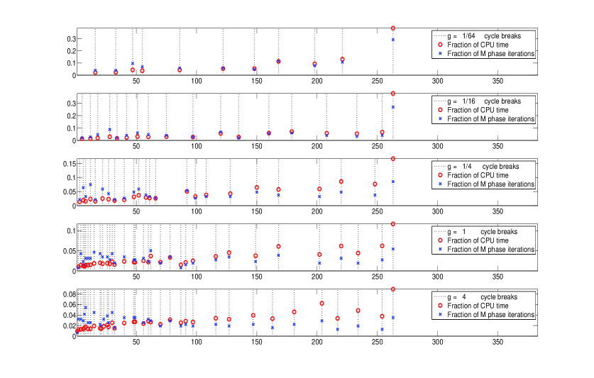
Figure 2: Some properties of the SMC algorithm in the cars example $\left(J=40,N=2500\right)$

Essentially by design, the algorithm achieves similar accuracy of approximation for all five prior distributions. For moments, this is driven by the iterations in the final $M$ phase that terminate only when the RNE for all monitoring functions first exceeds 0.9. The monitoring functions are not the same as the log-odds ratio functions of interest, and log marginal likelihood is not a posterior moment, but the principle that computation goes on until a prescribed criterion of numerical accuracy is achieved is common to all models and applications. Relative numerical efficiencies show less variation across the five cases for the large SPS executions for the usual reason: one learns more about reliability from $J=40$ particle groups than from $J=10$ particle groups.

The most striking feature of Table 2 is that more diffuse prior distributions (e.g., $g=1$, $g=4$) lead to more cycles and total iterations in the $M$ phase than do tighter prior distributions (e.g. $g=1/64$, $g=1/16$). Indeed, the ratio of $M$ phase iterations to cycles remains roughly constant. The key to understanding this behavior is the insight that the algorithm terminates the addition of information in the $C$ phase, thus defining a cycle, when the accumulation of new information has introduced enough variation in particle weights that effective sample size drops below the threshold of half the number of particles.

Figures 1 and 2 show the cycle breakpoints under each of the five prior distributions. Breakpoints tend to be more frequent near the start of the sample and algorithm, when the relative contribution of each observation to the posterior distribution is greatest. This is true in all five cases. As the prior distribution becomes more diffuse the posterior becomes more sensitive to each observation. This sensitivity is concentrated at the start of the sample and algorithm.

Later in the sample changes in the weight function are driven more by particular observations that contribute more information. These are the observations that are less likely conditional on previous observations, contributing to greater changes in the posterior distribution and therefore increasing the variation in particle weights and triggering new cycles. This is evident in breakpoints that are the same under all five prior distributions.

Consequently, the additional cycles and breakpoints arising from more diffuse priors tend to be concentrated in the earlier part of the algorithm. Sample sizes are smaller here than later, and the repeated evaluations of the likelihood function in the $M$ phase demand fewer computations. This is the main reason that relative computation time increase by a factor of less than 2, in moving from the tightest to the most diffuse prior in Table 3 , whereas the number of cycles and $M$ phase iterations more than triples.

The limiting cases are simple and instructive. A dogmatic prior implies a uniform weight function and one cycle. For most likelihood functions, in the limit a sequence of increasingly diffuse priors guarantees $t_{1}=1$, the existence exactly one unique particle in each group at the conclusion of the first $S$ phase, and therefore $\mathrm{rank}\left(V_{11}\right)=\min\left(J,\dim\left(\theta\right)\right)$ in the $M$ phase, and the algorithm will fail at step 2(c)i.

While the theory requires only that the prior distribution be proper, the SPS algorithm functions best for prior distributions that are seriously subjective – for example, the prior distribution developed in Section 3.1. This requirement arises from the representation of the Bayesian updating procedure by means of a finite number of points. Our experience in this and other models is that a proper prior distribution with a reasoned substantive interpretation presents no problems for the SPS algorithm. The next section illustrates this point.

5 Comparison of algorithms

We turn now to a systematic comparison of the efficiency and reliability of the PSW and SPS algorithms in the logit model.

5.1 The exercise

To this end, we simulated the posterior distribution for the Cartesian product of the eight data sets described in Section 3.2 and Table 1, the five prior distributions utilized in Section 4.2 and Table 3, and five approaches to simulation. The first approach to posterior simulation is the PSW algorithm implemented as described in Section 3.3. The second approach uses the small SPS simulation ($J=10$, $N=1000$) with the CPU implementation described in Section 3.3, and the third approach uses the GPU implementation. The fourth and fifth approaches are the same as the second and third except that they use the large SPS simulation ($J=40$, $N=2500$).

To complete this exercise we had to modify the multinomial logit model (last four data sets) for the PSW algorithm. The code that accompanies the algorithm requires that the vectors $\theta_{c}$ be independent in the prior distribution, and consequently (18) was modified to specify $\mathrm{cov}\left(\theta_{j}-\theta_{c},\theta_{i}-\theta_{c}\right)=0$. As a consequence, posterior moments approximated by the PSW algorithm depend on the normalization employed and are never the same as those approximated by the SPS algorithms. We utilized the same normalization as in the SPS algorithms, except for the cars data set, for which the code would not execute with this choice and we normalized instead on the second choice.

Table 4: Log marginal likelihoods, all data sets and models

	$g=1/64$	$g=1/16$	$g=1/4$	$g=1$	$g=4$
Diabetes	-405.87 [0.04]	-386.16 [0.03]	-383.31 [0.03]	-387.01 [0.04]	-392.61 [0.04]
Heart	-141.00 [0.04]	-123.36 [0.03]	-118.58 [0.04]	-124.38 [0.06]	-135.25 [0.11]
Australia	-301.87 [0.04]	-269.90 [0.05]	-267.41 [0.06]	-280.47 [0.07]	-300.20 [0.12]
Germany	-539.46 [0.06]	-535.91 [0.08]	-556.71 [0.00]	-586.66 [0.00]	-621.53 [0.00]
Cars	-263.75 [0.02]	-254.42 [0.03]	-253.62 [0.03]	-257.18 [0.03]	-262.20 [0.04]
Caesarean 1	-214.50 [0.03]	-187.19 [0.03]	-176.96 [0.02]	-177.29 [0.03]	-181.66 [0.03]
Caesarean 2	-219.20 [0.03]	-192.10 [0.03]	-180.30 [0.02]	-178.91 [0.02]	-181.42 [0.02]
Transportation	-234.58 [0.03]	-197.07 [0.04]	-176.14 [0.05]	-173.97 [0.05]	-184.24 [0.07]

Since it is impractical to present results from all $8\times 5\times 5=200$ posterior simulations, we restrict attention to a single prior distribution for each data set: the one producing the highest marginal likelihood. Table 4 provides the log marginal likelihoods under all five prior distributions for all eight data sets, as computed using the large SPS/GPU algorithm.

Note that the accuracy of these approximations is very high, compared with existing standards for posterior simulation. The accuracy of log-marginal likelihood approximation tends to decline with increasing sample size, as detailed in Durham and Geweke (2012, Section 4) and this is evident in Table 4. Going forward, all results pertain to the g-prior described in Section 3.1 with $g=1/16$ for Germany, $g=1$ for Caesarean 1 and transportation, and $g=1/4$ for the other five data sets.

Table 5: Posterior moments and numerical accuracy

		$(J=10,N=1000)$		$J=40,N=2500)$
	PSW	SPS/CPU	SPS/GPU	SPS/CPU	SPS/GPU
Diabetes	-0.853 (.096)	-0.855 (.095)	-0.852 (.096)	-0.853 (.095)	-0.853 (.095)
	[.0008, 0.68]	[.0009, 1.12]	[.0009, 1.21]	[.0003, 0.99]	[.0003, 1.03]
Heart	-0.250 (.192)	-0.246 (.187)	-0.251 (.191)	-0.249 (.189)	-0.250 (.189)
	[.0021, 0.43]	[.0019, 0.96]	[.0019, 0.98]	[.0006, 0.86]	[.0006, 0.92]
Australia	-0.438, .157)	-0.438 (.157)	-0.439 (.156)	-0.440 (.156)	-0.438 (.157)
	[.0023, 0.23]	[.0016, 0.96]	[.0016, 0.98]	[.0005, 0.97]	[.0006, 0.60]
Germany	-1.182 (.089)	-1.180 (.089)	-1.81 (.089)	-1.182 (.089)	-1.81 (.088)
	[.0010, 0.36]	[.0009, 1.00]	[.0004, 0.94]	[.0003, 0.91]	[.0004, 0.94]
Cars	-1.065 (.171)	0.684 (.156)	0.685 (.158)	0.685 (.156)	0.685 (.156)
	[.0002, 0.46]	[.0015, 1.03]	[.0017, 0.98]	[.0005, 1.12]	[.0005, 0.97]
	-0.665 (.156)	-0.386 (.195)	-0.388 (.195)	-0.387 (.194)	-0.388 (.193)
	[.0009, 0.60]	[.0021, 0.83]	[.0017, 1.29]	[.0006, 1.19]	[.0007, 0.72]
Caesarean 1	-1.975 (.241)	-2.049 (.245)	-2.052 (.248)	-2.052 (.246)	-2.052 (.246)
	[.0004, 0.26]	[.0024, 1.09]	[.0037, 0.45]	[.0008, 0.91]	[.0008, 0.96]
	-1.607 (.211)	-1.698 (.215)	-1.694 (.217)	-1.697 (.219)	-1.698 (.219)
	[.0003, 0.27]	[.0018, 1.36]	[.0024, 0.80]	[.0007, 1.07]	[.0006, 1.30]
Caesarean 2	-2.033 (.261)	-2.057 (.264)	-2.056 (.264)	-2.056 (.262)	-2.0534 (.262)
	[.0004, 0.22]	[.0027, 0.94]	[.0025, 1.32]	[.0008, 0.99]	[.0009, 0.89]
	-1.586 (.205)	-1.597 (.210)	-1.587 (.206)	-1.593 (.206)	-1.593 (.207)
	[.0003, 1.30]	[.0021, 0.98]	[.0021, 0.99]	[.0006, 1.02]	[.0006, 1.03]
Transportation	0.091 (.316)	0.130 (.321)	0.119 (.322)	0.123 (.322)	0.123 (.323)
	[.0006, 0.13]	[.0031, 1.09]	[.0030, 1.14]	[.0010, 1.01]	[.0010, 0.97]
	-0.588 (.400)	-0.416 (.380)	-0.416 (.388)	-0.421 (.386)	-0.419 (.388)
	[.0009, 0.09]	[.0020, 3.52]	[.0043, 0.82]	[.0012, 1.04]	[.0011, 1.29]
	-1.915 (.524)	-1.646 (.487)	-1.642 (.490)	-1.645 (.491)	-1.647 (.492)
	[.0013, 0.07]	[.0036, 1.84]	[.0044, 1.24]	[.0016, 0.95]	[.0019, 0.65]

5.2 Reliability

We assess the reliability of the algorithms by comparing posterior moment and marginal likelihood approximations for the same model. Table 5 provides the posterior moment approximations. The moment used is, again, the posterior expectation of the log-odds ratio(s) evaluated at the sample mean $\overline{x}$, for each choice relative to the last choice. (This corresponds to the normalization used in execution.) Thus there is one moment for each of the four binomial logit data sets, two moments for the first three multinomial logit data sets, and three moments for the last multinomial logit model data set.

The result for each moment and algorithm is presented in a block of four numbers. The first line has the simulation approximation of the posterior expectation followed by the simulation approximation of the posterior standard deviation. The second line contains [in brackets] the numerical standard error and relative numerical efficiency of the approximation. For the multinomial logit model there are multiple blocks, one for each posterior moment.

For the SPS algorithms the numerical standard error and relative numerical efficiency are the natural by-product of the results across the $J$ groups of particles as described in Section 2.1. For the PSW algorithm these are computed based on the 100 independent executions of the algorithm. The PSW approximations of the posterior expectation and standard deviation are based on a single execution.

Posterior moment approximations are consistent across algorithms. For the PSW algorithms there are $6\times 13=78$ pairwise comparisons of posterior expectations that can be made, and of these two are in the upper 1% or lower 1% tail of the distribution. The PSW moment approximations are consistent with the SPS moment approximations for the binomial logit data sets. As explained earlier in this section, the moments approximated by the PSW algorithm are not exactly the same as those approximated by the SPS algorithms in the last four data sets.

Table 6 compares approximations of log marginal likelihoods across the four variants of the SPS algorithm, and there are no anomalies. (The PSW algorithm does not yield approximations of the marginal likelihood.) There is no evidence of unreliability of any of the algorithms in Tables 5 and 6.

Table 6: Log marginal likelihoods and numerical accuracy

	$(J=10,N=1000)$		$J=40,N=2500)$
	SPS/CPU	SPS/GPU	SPS/CPU	SPS/GPU
Diabetes	-383.15 [0.05]	-383.14 [0.17]	-383.31 [0.03]	-383.25 [0.03]
Heart	-118.29 [0.15]	-118.73 [0.14]	-118.58 [0.04]	-118.61 [0.04]
Australia	-267.25 [0.32]	-267.35 [0.19]	-267.41 [0.06]	-267.35 [0.05]
Germany	-536.05 [0.21]	-536.10 [0.18]	-535.91 [0.08]	-535.89 [0.07]
Cars	-253.57 [0.07]	-253.46 [0.10]	-253.62 [0.03]	-253.61 [0.03]
Caesarean 1	-177.06 [0.08]	-176.72 [0.13]	-176.96 [0.02]	-176.91 [0.03]
Caesarean 2	-178.89 [0.08]	-178.95 [0.03]	-178.91 [0.02]	-178.83 [0.03]
Transportation	-174.09 [0.12]	-173.92 [0.19]	-173.97 [0.05]	-173.99 [0.05]

5.3 Computational efficiency

Our comparisons are based on a single run of each of the five algorithms (PSW and four variants of SPS) for each of the eight data sets, using for each data set one particular prior distribution chosen as indicated in Section 5.1. In the case of the PSW algorithm, we used 20,000 iterations for posterior moment approximation for the first four data sets, and 21,000 for the latter four data sets. The entries show wall-clock time for execution on the otherwise idle machine described in Section 3.3.  Execution time for the PSW algorithm 1,000 burn-in iterations in all cases except Australia and Germany, which have 5,000 burn-in iterations. Times can very considerably, depending on the particular hardware used: for example, the SPS/CPU algorithms were executed using a 12-core machine that utilized about 5 cores, simultaneously, on average; and the SPS/GPU algorithms used only a single GPU with 480 cores. The results here must be qualified by these considerations. We suspect that in practice the SPS/CPU algorithm might be slower for many users who have fewer CPU cores; and the SPS/GPU algorithm might be considerably faster with more GPUs.

Table 7: Clock execution time

		$(J=10,N=1000)$		$J=40,N=2500)$
	PSW	SPS/CPU	SPS/GPU	SPS/CPU	SPS/GPU
Diabetes	14.90	106.7	6.00	739.9	26.9
Heart	9.53	140.8	13.7	923.4	73.6
Australia	41.60	1793.5	69.2	12449.9	448.7
Germany	125.59	5910.4	225.9	45263.2	1689,4
Cars	7.62	33.5	3.5	231.2	18.9
Caesarean 1	6.84	97.3	10.9	723.3	55.3
Caesarean 2	6.65	15.2	2.5	133.3	11.6
Transportation	15.10	569.7	39.7	3064.2	293.7

Execution time also depends on memory management, clearly evident in Table 7. The ratio of execution time for the SPS/CPU algorithm in the large simulations ($J=40,N=2500$)  to that in the small simulations ($J=10,N=1000$) ranges from from 8.5 (Transportation) to 16.2 (Australia).  There is no obvious pattern or source for this variation, which we are investigating further.  The same ratio for the SPS/GPU algorithm ranges from 4.48 (Diabetes) to about 7.45 (Germany and Transportation). This reflects the fact that GPU computing is more efficient to the extent that the application is intensive in arithmetic logic as opposed to flow control. Very small problems are relatively inefficient; as the number and size of particles increases, the efficiency of the SPS/GPU algorithm increases, approaching an asymptotic ratio of number and size of particles to computing time from below.

Relevant comparisons of computing time $t$ require that we correct for the number $\widetilde{M}$ of iterations or particles and the relative numerical efficiency $R\widetilde{N}E$ of the algorithm. This produces an efficiency-adjusted computing time $\widetilde{t}=t/\left(\widetilde{M}\cdot R\widetilde{N}E\right)$. For $R\widetilde{N}E\$we use the average of the relevant RNE’s reported in Table 5: in the case of SPS, the averages are taken across all four variants since population RNE does not depend on the number of particles, hardware or software. This ignores variation in RNE from moment to moment and one run to the next. In the case of PSW, it also ignores dependence of RNE and number of burn-in iterations on the number of iterations used for moment approximations that arises from both practical and theoretical considerations. Therefore efficiency comparisons should be taken as indicative rather than definitive: they will vary from application to application in any event, and one will not undertake these comparisons for every (if indeed any) substantive study.

Table 8 provides the ratio of $\widetilde{t}$ for each of the SPS algorithms to $\widetilde{t}$ for the PSW algorithm, for each of the eight data sets. The SPS/CPU algorithm compares more favorably with the PSW algorithm for the small simulation exercises than for the large simulation exercises.  The SPS/CPU algorithm is clearly slower than the PSW algorithm, and its disadvantage becomes more pronounced the greater the number of parameters and observations.  With a single exception (Germany) the SPS/GPU algorithm is faster than the PSW algorithm for the large simulation exercises, and for the single exception it is about 2% slower.

Table 8: Computational efficiency relative to PSW

	$(J=10,N=1000)$		$J=40,N=2500)$
	SPS/CPU	SPS/GPU	SPS/CPU	SPS/GPU
Diabetes	9.40	0.53	6.52	0.24
Heart	14.35	1.40	9.41	0.75
Australia	28.25	1.09	19.61	0.71
Germany	45.06	1.72	34.51	1.29
Cars	5.04	0.53	3.47	0.28
Caesarean 1	8.36	0.94	6.21	0.47
Caesarean 2	3.73	0.62	3.28	0.29
Transportation	6.19	0.43	3.33	0.32

6 Conclusion

The class of sequential posterior simulation algorithms is becoming an important subset of the computational tools that Bayesian statisticians have at their disposal in applied work. Graphical processing units, in turn, have become a convenient and very cost-effective platform for scientific computing, potentially accelerating computing speeds by orders of magnitude for suitable algorithms. One of the appealing features of SPS is the fact that it is almost ideally suited for GPU computing. Here we have used an SPS algorithm developed specifically in Durham and Geweke (2012) to exploit that potential.

The multinomial logistic regression model, the focus of this paper, is important in applied statistics in its own right, and also as a component in mixture models, Bayesian belief networks, and machine learning. The model presents a well conditioned likelihood function that renders maximum likelihood methods straightforward, yet it has been relatively difficult to attack with posterior simulators – and hence arguably a bit of an embarrassment for applied Bayesian statisticians. Recent work by Frühwirth and Frühwirth-Schnatter (2007, 2012), Holmes and Held (2006), Scott (2011) and, especially, Polson et al. (2012) has improved this state of affairs substantially, using latent variable representations specific to classes of models that include the multinomial logit.

The SPS algorithm of Durham and Geweke (2012), implemented using Matlab and a single GPU, led to computation time in the range of 10% to 100% of the computation time required by the algorithm of Polson et al. (2012), which in turn appears to be the most computationally efficient of alternative algorithms. Using Matlab and a multicore CPU, the comparison is (very roughly) reversed, with the algorithm of Polson et al. (2012) having computation time in the range of 10% to 100% of the SPS algorithm But given the low cost of GPUs – on the order of US$250, and the possibility of having up to 8 GPU’s in a single convention desktop machine – together with the efficiency of user-friendly software like Matlab, there are no essential obstacles in moving to GPU computing for applied Bayesian statisticians. Indeed, some of the case studies are too small to fully exploit the power of this new platform, as evident in increased efficiency for SPS/GPU with $10^{5}$ particles as opposed to $10^{4}$ particles.

The SPS algorithm has other attractions that are as significant as computational efficiency. These advantages are generic, but some are more specific to the logit model than others.

1. SPS produces an accurate approximation of the log marginal likelihood as a by-product. The latent variable algorithms, including all of those just mentioned, do not. SPS also produces accurate approximations of log predictive likelihoods, a significant factor in time series models.

2. SPS approximations have a firm foundation in distribution theory. The algorithm produces a reliable approximation of the standard deviation in the applicable central limit theorem – again, as a by-product in the approach developed in Durham and Geweke (2012). Numerical accuracy in the latent variable methods for posterior simulation do not do this, and we are not aware of procedures for ascertaining reliable approximations of accuracy with these methods that do not entail a significant lengthening of computation time.

3. More generally, SPS is simple to implement when the likelihood function can be evaluated in closed form. Indeed, in comparison with alternatives it can be trivial, and this is the case for the logit model studied in this paper. By implication, the time from conception to Bayesian implementation is greatly reduced for this class of models.

4. The ease of implementation, combined with the speed of execution of the SPS algorithm in a GPU and user-friendly environment, renders the case for compromises with exact likelihood methods due to exigencies of application less tenable overall. The same can be said for compromises with exact subjective Bayesian inference.

References

Albert JH, Chib S (1993). Bayesian analysis of binary and polychotomos response data. Journal of the American Statistical Association 88: 669-679.

Andrieu C, Doucet A, Holenstein A (2010). Particle Markov chain Monte Carlo. Journal of the Royal Statistical Society, Series B 72: 1–33.

Baker JE (1985). Adaptive selection methods for genetic algorithms. In Grefenstette J (ed.), Proceedings of the International Conference on Genetic Algorithms and Their Applications, 101–111. Malwah NJ: Erlbaum.

Baker JE (1987). Reducing bias and inefficiency in the selection algorithm. In Grefenstette J (ed.) Genetic Algorithms and Their Applications, 14–21. New York: Wiley.

Chopin N (2002). A sequential particle filter method for static models. Biometrika 89: 539–551.

Chopin N (2004). Central limit theorem for sequential Monte Carlo methods and its application to Bayesian inference. Annals of Statistics 32: 2385-2411.

Chopin N, Jacob PI, Papaspiliopoulis O (2011). SMC²: A sequential Monte Carlo algorithm with particle Markov chain Monte Carlo updates. Working paper. http://arxiv.org/PS_cache/arxiv/pdf/1101/1101.1528v2.pdf

Del Moral P, Doucet A, Jasra A (2011). On adaptive resampling strategites for sequential Monte Carlo methods. Bernoulli 18: 252-278.

Durham G, Geweke J (2012). Adaptive Sequential Posterior Simulators for Massively Parallel Computing Environments. http://www.censoc.uts.edu.au/pdfs/geweke_ papers/gpu2_full.pdf.

Fahrmeilr L, Tutz G (2001). Multivariate Statistical Modeling based on Generalized Linear Models. Springer.

Foster DP, Stine RA, Waterman RP (1998). Business analysis using regression. Springer.

Flegal JM, Jones GL (2010). Batch means and spectral variance estimators in markov chain Monte Carlo. Annals of Statistics 38: 1034-1070.

Frühwirth-Schnatter S, Frühwirth, R (2007). Auxiliary mixture sampling with applications to logistic models. Computational Statistics and Data Analysis 51: 3509 – 3582.

Frühwirth-Schnatter S, Frühwirth, R (2012). Bayesian inference in the multinomial logit model. Austrian Journal of Statistics 41: 27-43.

Geweke J, Keane M (2007). Smothly mixing regressions. Journal of Econometrics 138: 252-290.

Geweke J, Keane M, Runkle D (1994). Alternative computational approachesto inference in the multinomial probit mdoel. Review of Economics and Statistics 76: 609-632.

Gordon NJ, Salmond DJ, Smith AFM (1993). Novel approach to nonlinear / non-Gaussian Bayesian state estimation. IEEE Proceedings F on Radar and Signal Processing 140 (2): 107-113.

Gramacy RB, Polson NG (2012). Simulation-based regularized logistic regression. Bayesian Analysis 7: 567-589.

Green WH (2003). Econometric Analysis. Fifth Edition. Prentice-Hall.

Herbst E, Schorfheide F (2012). Sequential Monte Carlo sampling for DSGE models. http://www.ssc.upenn.edu/~schorf/papers/smc_paper.pdf

Holmes C, Held L (2006). Bayesian auxiliary variable models for binary and multinomial regression. Bayesian Analysis 1: 145-168.

Jacobs RA, Jordan MI, Nowlan SJ (1991). Adaptive mixtures of local experts. Neural Computation 3: 79-87.

Jiang WX, Tanner MA (1999).Hierarchical mixtures-of-experts for exponential family regression models: Approximation and maximum likelihood estimation. Annals of Statistics 27: 987-1011.

Kong A, Liu JS, Wong WH (1994). Sequential imputations and Bayesian missing data problems. Journal of the American Statistical Association 89:278–288.

Liu JS, Chen R (1995). Blind deconvolution via sequential imputations. Journal of the American Statistical Association 90: 567–576.

Liu JS, Chen R (1998). Sequential Monte Carlo methods for dynamic systems. Journal of the American Statistical Association 93: 1032–1044.

Polson NG, Scot JG, Windle J (2012). Bayesian inference for logistic models using Polya-Gamma latent variables. http://faculty.chicagobooth.edu/nicholas.polson /research/papers/polyaG.pdf

Scott SL (2011). Data augmentation, frequentist estimation, and the Bayesian analysis of multinomial logit models. Statistical Papers 52; 87-109.

Zellner A (1986). On assessing prior distributions and Bayesian regression analysis with g-prior distributions. In: Goel P, Zellner A (eds.), Bayesian Inference and Decision Techniques: Studies in Bayesian Econometrics and Statististics. 6 233–243. North-Holland.