An Algorithm for Computing Constrained Reflection Paths in Simple Polygons

Abstract

Let $s$ be a source point and $t$ be a destination point inside an $n$-vertex simple polygon $P$. Euclidean shortest paths [Lee and Preparata, Networks, 1984; Guibas et al. , Algorithmica, 1987] and minimum-link paths [Suri, CVGIP, 1986; Ghosh, J. Algorithms, 1991] between $s$ and $t$ inside $P$ have been well studied. Both these kinds of paths are simple and piecewise-convex. However, computing optimal paths in the context of diffuse or specular reflections does not seem to be an easy task. A path from a light source $s$ to $t$ inside $P$ is called a diffuse reflection path if the turning points of the path lie in the interiors of the boundary edges of $P$. A diffuse reflection path is said to be optimal if it has the minimum number of turning points amongst all diffuse reflection paths between $s$ and $t$. The minimum diffuse reflection path may not be simple. The problem of computing the minimum diffuse reflection path in low degree polynomial time has remained open.

In our quest for understanding the geometric structure of the minimum diffuse reflection paths vis-a-vis shortest paths and minimum link paths, we define a new kind of diffuse reflection path called a constrained diffuse reflection path where (i) the path is simple, (ii) it intersects only the eaves of the Euclidean shortest path between $s$ and $t$, and (iii) it intersects each eave exactly once. For computing a minimum constrained diffuse reflection path from $s$ to $t$, we present an $O(n(n+\beta))$ time algorithm, where $\beta=\Theta(n^{2})$ in the worst case. Here, $\beta$ depends on the shape of the polygon. We also establish some properties relating minimum constrained diffuse reflection paths and minimum diffuse reflection paths. Constrained diffuse reflection paths introduced in this paper provide new geometric insights into the hitherto unknown structures and shapes of optimal reflection paths. Our algorithm demonstrates how properties like convexity, simplicity, complete visibility, etc., can be combined in computing and understanding diffuse reflection paths that are optimal or close to optimal.

• diffuse reflection, simple polygon, minimum diffuse reflection path, visibility, constrained diffuse reflection path

1 Introduction

1.1 Visibility and reflections

Problems of direct visibility have been studied extensively in the last few decades (see [10]). Let $P$ be an $n$-vertex simple polygon where $int(P)$ and $bd(P)$ denote the interior and boundary of $P$, respectively. Two points inside a polygon $P$ are said to be $visible$ (directly) if the line segment joining them lies totally inside $int(P)\cup bd(P)$. The region of $P$ visible directly from a point light source $s$ in $P$ is called the visibility polygon of $P$ from $s$ (see Figure 1). Efficient algorithms have been designed for computing visibility polygons under various conditions [10]. Note that some points of $P$ that are not directly visible or illuminated from $s$, can become visible due to multiple reflections on the edges of $P$ (see Figure 1).

We are interested in computing the visibility of a point from $s$ by multiple reflections inside $P$; the sequence of multiple reflections is simply a reflection path. Reflections are of two types – specular and diffuse. As per the law of reflection, the reflection of a light ray at a point is called specular if the angle of incidence is equal to the angle of reflection. The other type of reflection of light is called diffuse reflection that happens for most reflecting surfaces. Here, a ray incident at a point of an edge $e$ is reflected in all possible interior directions except along the edge $e$. We assume that all edges of $P$ can reflect in this manner. We also assume that any ray of light incident at a vertex is absorbed and not reflected.

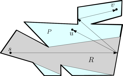
Figure 1: The region $R$ is directly visible from $s$. A ray from $s$ reaches $u$ after one specular reflection. A ray from $s$ reaches $v$ after two diffuse reflections.

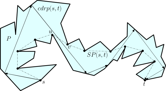
Figure 2: A $cdrp(s,t)$ intersects only eaves of $SP(s,t)$.

Multiple reflections arise naturally in the realistic rendering of three-dimensional scenes [1, 7, 8, 11]. In rendering of images by ray-tracing, light sources reachable by a small number of reflections through an image pixel would contribute intensely at the pixel because of limited loss of intensity at each stage of reflection. Computing diffuse reflection paths of light arriving from a light source by a small number of reflections (or turning points) is therefore, an important problem. In this paper we focus on the polynomial time computation of certain constrained paths of multiple diffuse reflections. Prior works on visibility with multiple reflections are reviewed in Section 2.

1.2 Euclidean shortest path and minimum link path

A polygonal path is said to be simple if it is not self intersecting. Henceforth, we use the term path instead of polygonal path. A path from $s$ to $t$ inside $P$ is said to be convex if it makes only unidirectional turns (either left or right) while traversing from $s$ to $t$. If the turns are always right (or, left) turns, the path is right convex (respectively, left convex). A path from $s$ to $t$ inside $P$ is said to be piecewise-convex if it can be broken into alternating sequences of left and right convex paths.

Let $SP(s,t)$ denote the Euclidean shortest path, the path of the shortest length, from $s$ to $t$ inside $P$. Let $uv$ be an edge of $SP(s,t)$ such that if $P$ is cut along $uv$, then $s$ and $t$ belong to the two different subpolygons of $P$ (see Figure 2). Such an edge $uv$ is called an eave [10]. Notice that $uv$ is a diagonal of $P$. $SP(s,t)$ is simple and piecewise convex with reversal of turns at eaves.

A minimum link path [9, 17] between two points $s$ and $t$ (denoted as $mlp(s,t)$) is a polygonal path inside $P$ having the minimum number of turns. Like $SP(s,t)$, $mlp(s,t)$ is also simple and piecewise convex. Moreover, $mlp(s,t)$ intersects $SP(s,t)$ only at eaves and each eave is intersected exactly once [10]. The number of links in a minimum link path between any two points of $P$ is called the link distance between them.

1.3 Diffuse reflection paths

As stated earlier, reachability problems in terms of Euclidean shortest paths and minimum link paths between a source point $s$ and a destination point $t$ inside a simple polygon $P$ have been well studied [10]. In this paper, we seek to compute a special class of optimal diffuse reflection paths that are analogous to $SP(s,t)$ and $mlp(s,t)$. We call such paths constrained diffuse reflection paths which we define next.

A diffuse reflection path $drp(s,t)$ from $s$ to $t$ is a path inside $P$ from $s$ to $t$ such that the turns of the path are in the interiors of the edges of $bd(P)$. Note that every $drp(s,t)$ must intersect all the eaves of $SP(s,t)$. If all turning points of a $mlp(s,t)$ lie on $bd(P)$, then $mlp(s,t)$ is a $drp(s,t)$. A $drp(s,t)$ is said to be optimal if it has the minimum number of reflections amongst all diffuse reflection paths between $s$ and $t$. An optimal $drp(s,t)$ can always be computed in exponential time [16]. Aronov et al. [3] claimed that the combinatorial complexity of the visible region after $k$ diffuse reflections is $O(n^{9})$, for any $k\leqslant n$. It seems that this result may be used for computing an $mdrp(s,t)$ in very high order polynomial time but no explicit procedure is stated in the paper. Designing a low degree polynomial time algorithm for computing an $mdrp(s,t)$ remains open. In Section 2, we state the known approximation algorithms for computing $drp(s,t)$.

A $drp(s,t)$ is said to be constrained if (i) it is simple, (ii) it intersects only the eaves of $SP(s,t)$, and (iii) it intersects each eave exactly once. Such a path is denoted by $cdrp(s,t)$; see Figure 2 for an illustration. If every $drp(s,t)$ intersects itself or intersects a non-eave edge of $SP(s,t)$, then there cannot exist a $cdrp(s,t)$. In Figure 3, any $cdrp(s,t)$ has to enter triangle $abc$ from $ab$ and exit from $bc$. Such a $cdrp(s,t)$ must end up on the clockwise polygonal boundary from $f$ to $g$ and therefore, can not reach $t$, where $f$ is the extension of $ab$ to $bd(P)$ and $g$ is the extension of $bc$ to $bd(P)$.

If a $cdrp(s,t)$ has the minimum number of turns amongst all $cdrp(s,t)$, then it is denoted as $mcdrp(s,t)$. Ghosh [9, 10] showed how $SP(s,t)$ can be transformed into a $mlp(s,t)$ in $P$. Following a similar approach as shown in the sequel, $SP(s,t)$ can also be transformed to a $cdrp(s,t)$ (if it exists). In addition, they all have the same number of reversals of turns from $s$ to $t$ only at eaves; the turns immediately before and after each link crossing an eave have reverse directions, just as the turns at the two end of an eave in $SP(s,t)$ have reverse directions. Thus, one can observe that the particular diffuse reflection path we are interested in has significant structural similarities with the Euclidean shortest paths and the minimum link paths.

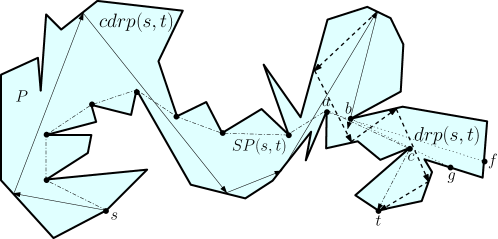
Figure 3: There is no $cdrp(s,t)$ as any path must intersect non-eave edge of $SP(s,t)$.

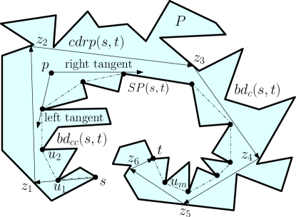
Figure 4: Every $cdrp(s,t)$ is a convex and simple path.

Section 2 reviews previous work on visibility with multiple reflections. The main goal of this paper is to compute an optimal constrained diffuse reflection path $mcdrp(s,t)$ that is dealt with in Section 3. We present an $O(n(n+\beta))$ time algorithm for computing $mcdrp(s,t)$. Here, $\beta=\Theta(n^{2})$ depends on the shape of the polygon. To the best of our knowledge, this is the first attempt at computing any class of optimal diffuse reflection path. Section 4 relates $mcdrp(s,t)$ with $drp(s,t)$ and Section 5 concludes the paper.

2 Previous results

We state some known results on visibility with multiple reflections. In [2], Aronov et al. studied the region visible from a point source inside a simple $n$-vertex polygon where at most one specular (or diffuse) reflection is permitted on the bounding edges. They established a tight $\Theta(n^{2})$ worst-case combinatorial complexity bound for the region visible after at most one reflection. They also proposed an algorithm for computing such regions in $O(n^{2}\log^{2}n)$ time for both specular as well as diffuse reflections. Aronov et al. [1] addressed the general problem where at most $k\geqslant 2$ specular reflections are used. An upper bound of $O(n^{2k})$ and a worst-case lower bound of $\Omega((n/k)^{2k})$ was established on the combinatorial complexity of the region visible due to at most a constant number $k$ of specular reflections. They also proposed an algorithm running in $O(n^{2k}\log n)$ time, for $k>1$. Davis [6] studied several variations of reflection problems.

Prasad et al. [16] showed that the upper bound on the number of edges and vertices of the region visible due to at most $k$ diffuse reflections is $O(n^{2\lceil(k+1)/2\rceil+1})$. They designed an $O(n^{2\lceil(k+1)/2\rceil+1}\log n)$ time algorithm for computing such a visible region. In [16] they conjectured that the complexity of the region visible due to at most $k$ diffuse reflections is $\Theta(n^{2})$. Note that this region may contain blind spots or holes (see in [15]). Aronov et al. [3] claimed that the complexity of this visible region is $O(n^{9})$. Bridging the big gap between the $O(n^{9})$ upper bound of Aronov et al. [3], and the $\Omega(n^{2})$ lower bound as in [16], is an open problem.

Recently, Ghosh et al. [11] have presented three different algorithms for computing sub-optimal diffuse reflection paths from $s$ to $t$ inside $P$. For constructing such a path, the first algorithm uses a greedy method, the second algorithm uses a transformation of a minimum link path, and the third algorithm uses the edge-edge visibility graph of $P$. The first two algorithms are for simple polygons, and they run in $O(n+k\log n)$ time, where $k$ denotes the number of reflections in the constructed path. The third algorithm runs in $O(n^{2})$ time and works for polygons with or without holes. The number of reflections in the path produced by the third algorithm can be at most three times that in an optimal diffuse reflection path.

3 Computing an optimal constrained diffuse reflection path

Let $SP(s,t)=(s,u_{1},u_{2},\ldots,u_{m},t)$, where $u_{1},u_{2},\ldots,u_{m}$ are vertices of $P$. We know that $SP(s,t)$ can be computed in linear time [14]. Since $cdrp(s,t)$ intersects $SP(s,t)$ only at the eaves, all other edges of $SP(s,t)$ can be treated as polygonal edges. So, we assume without loss of generality, that $s$ and $t$ lie on $bd(P)$. We first present an algorithm for computing a $mcdrp(s,t)$ for the special case where no edge of $SP(s,t)$ is an eave (see Figure 4). Later we allow eaves in $SP(s,t)$.

3.1 $SP(s,t)$ has no eave

3.1.1 Characterizing the path $cdrp(s,t)$

We know that $SP(s,t)$ is either right convex or left convex as there is no eave. Without loss of generality, we assume that $SP(s,t)$ makes a right turn at every vertex of the path, while traversing from $s$ to $t$. So, vertices of $SP(s,t)$ belong to the counterclockwise boundary of $P$ from $s$ to $t$ (denoted as $bd_{cc}(s,t)$). Since a $cdrp(s,t)$ does not intersect any edge of $SP(s,t)$, all turning points of the $cdrp(s,t)$ lie on the clockwise boundary of $P$ from $s$ to $t$ (denoted as $bd_{c}(s,t)$). We have the following lemma that establishes the convexity property of $cdrp(s,t)$, as we have for $SP(s,t)$ and $mlp(s,t)$.

Lemma 1.

Every $cdrp(s,t)$ is a convex and simple path.

Proof.

Consider a $cdrp(s,t)=(s,z_{1},\ldots,z_{p},t)$ where $z_{i}$, $1\leqslant i\leqslant p$, are the turning points of the $cdrp(s,t)$ on $bd(P)$. Since the path is simple by definition, the next turning point $z_{i+1}$ of $z_{i}$ cannot belong to $bd_{c}(s,z_{i})$, for all $i$. Further, since $cdrp(s,t)$ does not intersect any edge of $SP(s,t)$, $z_{i+1}$ must belong to $bd_{c}(z_{i},t)$. Since each turning point $z_{i}$ of the $cdrp(s,t)$ is an interior point of an edge of $bd_{c}(s,t)$, the $cdrp(s,t)$ makes a right turn at $z_{i}$, for all $i$. Therefore, $cdrp(s,t)$ is a simple and convex path. ∎

Corollary 2.

The turning points $z_{1},z_{2},\ldots,z_{p}$ of $cdrp(s,t)=(s=z_{0},z_{1},\ldots,...,z_{p},z_{p+1}=t)$ appear in clockwise order along $bd_{c}(s,t)$.

For any point $p$ inside $P$, we say that the line segment $pu_{i}$ is a left (or, right) tangent from $p$ to $SP(s,t)$ at the vertex $u_{i}$ (see Figure 4), if both $u_{i-1}$ as well as $u_{i+1}$, lie to the left (respectively, right) of the ray emanating from $p$ through $u_{i}$. Note that $u_{i-1}$, $u_{i}$ and $u_{i+1}$ are consecutive vertices of $SP(s,t)$. We have the following lemma.

Lemma 3.

The right and left tangents from any turning point $z_{i}$ of a $cdrp(s,t)$ to $SP(s,t)$ lie entirely inside the simple polygon $P$.

Proof.

The proof follows from Lemma 1 due to the convexity and simplicity of the $cdrp(s,t)$. ∎

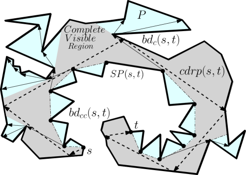
Figure 5: Every $cdrp(s,t)$ lies inside $CV(s,t)$.

Let $CV(s,t)$ be the complete visible region of $P$ bounded by $SP(s,t)$ and $bd_{c}(s,t)$ such that the right and left tangents from every point $z$ of $CV(s,t)$ to $SP(s,t)$, lie inside $P$ (see Figure 5). It follows from Lemma 3 that a $cdrp(s,t)$ lies totally inside $CV(s,t)$ with turning points on the polygonal edges belonging to $CV(s,t)$ as stated in the following lemma.

Lemma 4.

Every $cdrp(s,t)$ lies entirely inside $CV(s,t)$.

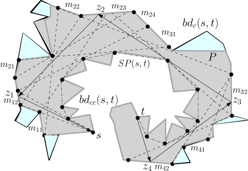
Figure 6: Mirrors $M_{1}=(m_{11},m_{12})$, $M_{2}=(m_{21},m_{22},m_{23},m_{24})$, $M_{3}=(m_{31},m_{32})$, $M_{4}=(m_{41},m_{42})$ are computed in clockwise order along $BCV(s,t)$.

The region $CV(s,t)$ can be computed in linear time by traversing the shortest path trees inside $P$ rooted at $s$ and $t$ as given in [5, 9, 10]. A shortest path tree rooted at a vertex $v$ is the union of the Euclidean shortest paths from $v$ to all vertices of $P$. The main property used by the algorithm in traversing the trees is given below.

Lemma 5.

[5, 9] Let $u$ and $w$ be the parents of a vertex $v\in bd_{c}(s,t)$ in the shortest path trees inside $P$ rooted at $s$ and $t$. The vertex $v$ belongs to $CV(s,t)$ if and only if both $u$ and $w$ belong to $SP(s,t)$.

3.1.2 Computing the reflecting edges for $cdrp(s,t)$

The above discussion shows that all the turning points of a $cdrp(s,t)$ must lie on edges of $bd_{c}(s,t)$ that also belong to $CV(s,t)$. We denote the sequence of such intervals on polygonal edges as $BCV(s,t)$ $=$ $bd(P)\cap CV(s,t)$. We refer to polygonal edges containing edges of $BCV(s,t)$ as reflecting edges. Let us first identify intervals of $BCV(s,t)$ on reflecting edges that can have the first turning point of a $cdrp(s,t)$. Let $M_{1}=(m_{11},m_{12},\ldots)$ be the intervals visible from $s$ on reflecting edges in clockwise order along $bd_{c}(s,t)$ (see Figure 6). We refer to these intervals as mirrors of $M_{1}$. If $t$ is visible from any point $z_{1}$ on a mirror of $M_{1}$, then $(s,z_{1},t)$ is a $cdrp(s,t)$.

Assume that $t$ is not visible from any mirror of $M_{1}$. We identify intervals on reflecting edges such that every point in any such interval is visible from some point in a mirror of $M_{1}$. Note that a point on a reflecting edge may be visible from points in two or more mirrors of $M_{1}$. For each reflecting edge, the union of such intervals gives disjoint intervals on that reflecting edge. Let $M_{2}=(m_{21},m_{22},\ldots)$ be the intervals or mirrors in clockwise order along $bd_{c}(s,t)$. Likewise, let $M_{i}=(m_{i1},m_{i2},\ldots)$ be the mirrors created from the set $M_{i-1}=(m_{(i-1),1},m_{(i-1),2},\ldots)$ of mirrors for $i\geqslant 3$. We have the following lemmas.

Lemma 6.

All mirrors of $M_{2}$ appear after all mirrors of $M_{1}$ in clockwise order along $BCV(s,t)$.

Proof.

Let $a$, $b$ and $c$ be three points on $bd_{c}(s,t)$ in clockwise order such that $a$ and $c$ are visible from $s$ but $b$ is not. In other words, $a$ and $c$ belong to two mirrors of $M_{1}$ but $b$ does not belong to any mirror of $M_{1}$. Assume that $b$ is visible from $a$. So, no part of $bd_{c}(s,t)$ between $a$ and $b$ can intersect $bs$. If $bd_{c}(s,t)$ between $b$ and $c$ intersects $bs$, then $b$ does not belong to $BCV(s,t)$. If $SP(s,t)$ intersects $bs$, then it also intersects $cs$, contradicting the assumption that $c$ is visible from $s$. So, the second turning point of a $cdrp(s,t)$ must be on subsequent reflecting edges of $M_{1}$ in clockwise order. ∎

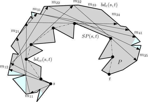
Figure 7: Mirrors of $M_{2}$, $M_{3}$ and $M_{4}$ are interleaved.

The above relation between mirrors $M_{1}$ and $M_{2}$ cannot be generalized for mirrors of $M_{2},M_{3},\ldots$, since mirrors in these sets may be interleaved as shown in Figure 7. On the other hand, we have the following properties relating mirrors of $M_{1},M_{2},M_{3},\ldots$ and turning points of any $cdrp(s,t)$.

Lemma 7.

No point on a mirror of $M_{i}$ is visible from any point on any mirror of $M_{1},\ldots,M_{i-2}$, for all $i\geqslant 3$.

Proof.

The proof follows from the definition of the mirrors $M_{i}$. ∎

Corollary 8.

If every turning point on a $cdrp(s,t)$ belongs to a distinct $M_{i}$, then this $cdrp(s,t)$ is an $mcdrp(s,t)$.

Proof.

If each of the $k$ turning points of a $cdrp(s,t)$ is from a distinct $M_{i}$, then due to Lemma 7, the turning points must be on mirrors of $M_{1}$, $M_{2}$, …, $M_{k}$, respectively. Therefore, the $cdrp(s,t)$ is also an $mcdrp(s,t)$. ∎

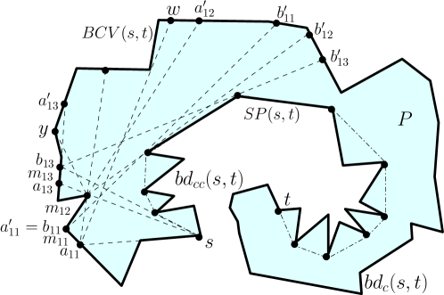
Figure 8: After locating $a^{\prime}_{11},a^{\prime}_{12},\ldots$ and $b^{\prime}_{11},b^{\prime}_{12},\ldots$ on $BCV(s,t)$, $M_{2}=(m_{21},m_{22},m_{23},\ldots)$ is computed from $M_{1}=(m_{11},m_{12},m_{13},\ldots)$. Note that $a_{12}$, $a^{\prime}_{11}$ and $b_{11}$ happen to be the same point in this figure.

We next discuss the computation of endpoints of mirrors of $M_{i}$ from the mirrors of $M_{i-1}$ for $i\geqslant 2$. A point $x\in BCV(s,t)$ is said to be weakly visible from a mirror if $x$ is visible from some point of the mirror. Consider the first mirror $m_{11}$ (see Figure 8). Let $a_{11}$ and $b_{11}$ be the endpoints of $m_{11}$, where $b_{11}$ is the subsequent clockwise point of $a_{11}$ on $BCV(s,t)$. Let $a^{\prime}_{11}$ be the first point in the clockwise order on a reflecting edge of $M_{2}$ that is visible from $a_{11}$. Similarly, let $b^{\prime}_{11}$ be the last point in the clockwise order on a reflecting edge of $M_{2}$ that is visible from $b_{11}$. Observe that if the right tangent from $b_{11}$ to $SP(s,t)$ is extended to $BCV(s,t)$, then it meets $BCV(s,t)$ at $b^{\prime}_{11}$. The portion of $bd_{c}(a^{\prime}_{11},b^{\prime}_{11})$ belonging to $BCV(s,t)$, and weakly visible from $m_{11}$ is called the span of $m_{11}$, and is denoted as $span(a^{\prime}_{11},b^{\prime}_{11})$. In the same way, the span of any mirror $m_{ij}$ can be defined. Observe that $b^{\prime}_{11}$, $b^{\prime}_{12}$, $b^{\prime}_{13},\ldots$ occur in clockwise order along $BCV(s,t)$.

From the above definitions, the mirrors of $M_{2}$ formed due to reflections on $m_{11}$ must belong to $span(a^{\prime}_{11},b^{\prime}_{11})$.

Let us identify mirrors of $M_{2}$ formed due to reflections on $m_{12}$. These mirrors are formed on $span(a^{\prime}_{12},b^{\prime}_{12})$, that is, on the portion of $bd_{c}(a^{\prime}_{12},b^{\prime}_{12})$ on $BCV(s,t)$, after excluding the portion $span(a^{\prime}_{11},b^{\prime}_{11})$. If $a^{\prime}_{12}\in span(a^{\prime}_{11},b^{\prime}_{11})$, it follows that mirrors of $M_{2}$ formed due to the reflection on $m_{12}$ must belong to the non-overlapping portion $bd_{c}(b^{\prime}_{11},b^{\prime}_{12})$, weakly visible from $m_{12}$ and on $BCV(s,t)$. If $span(a^{\prime}_{11},b^{\prime}_{11})$ and $span(a^{\prime}_{12},b^{\prime}_{12})$ are disjoint, then mirrors of $M_{2}$ formed due to reflections on $m_{12}$ belong to $span(a^{\prime}_{12},b^{\prime}_{12})$. If $span(a^{\prime}_{12},b^{\prime}_{12})$ contains $span(a^{\prime}_{11},b^{\prime}_{11})$, two weakly visible portions of $bd_{c}(a^{\prime}_{12},a^{\prime}_{11})$ and $bd_{c}(b^{\prime}_{11},b^{\prime}_{12})$ on $BCV(s,t)$, contain mirrors of $M_{2}$ formed due to reflections on $m_{12}$.

For identifying mirrors of $M_{2}$ formed due to reflections on $m_{13}$, remove $span(a^{\prime}_{11},b^{\prime}_{11})$ and $span(a^{\prime}_{12},b^{\prime}_{12})$ from $span(a^{\prime}_{13},b^{\prime}_{13})$. Mirrors of $M_{2}$ formed due to reflections on $m_{13}$ lie on the remaining portions of $span(a^{\prime}_{13},b^{\prime}_{13})$. Using this process of concatenations repeatedly, mirrors of $M_{2}$ can be identified from the spans of mirrors of $M_{1}$. Furthermore, mirrors of $M_{i}$ can be identified given mirrors of $M_{i-1}$ in a similar manner for $i\geqslant 3$.

Now we consider two kinds of mirrors possible on edges of $BCV(s,t)$. Some of these mirrors are side mirrors, ending at vertices of $BCV(s,t)$. The others are internal mirrors with endpoints in the interiors of edges of $BCV(s,t)$. In the following lemmas, we bound the number of mirrors using the maximum link distance (denoted as $\alpha(i)$) between any two points on the first and last mirrors of $M_{i}$, for all $i$.

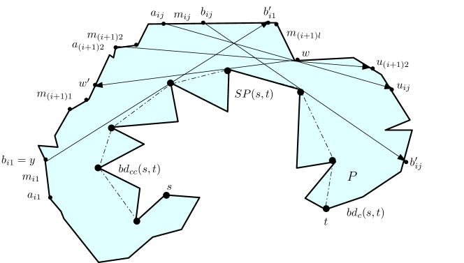
Figure 9: The vertex $w$ of $BCV(s,t)$ is visible from $m_{ij}$ and $m_{(i+1)2}$.

Lemma 9.

A vertex $w$ of $BCV(s,t)$ can be visible only from mirrors of $M_{i}$, $M_{i+1}$, $M_{i+2}\ldots$, $M_{i+\alpha(i)}$, where $i$ is the smallest index such that a mirror of $M_{i}$ sees $w$.

Proof.

Draw the left tangent from $w$ to $SP(s,t)$ and extend to $BCV(s,t)$ meeting it at a point $w^{\prime}$ (see Figure 9). All mirrors that can see $w$ must belong to $bd_{c}(w^{\prime},w)$. Locate the mirror $m_{qj}$ on $bd_{c}(w^{\prime},w)$ such that (i) $m_{qj}$ can see $w$, (ii) $q$ is the smallest among all mirrors on $bd_{c}(w^{\prime},w)$ that can see $w$, and (iii) $j$ is the smallest among all mirrors of $M_{q}$ on $bd_{c}(w^{\prime},w)$ that can see $w$. We set $i$ to $q$. We know that any $mcdrp(s,w)$, can have only one turning point on a mirror amongst all mirrors of $bd_{c}(w^{\prime},w)$ due to Lemma 7. We assume that at least one mirror of $M_{i}$ does not see $w$, e.g., the first mirror $m_{i1}$ of $M_{i}$. This is the case where $\alpha(i)=2$; the case where $\alpha(i)=1$ is simpler because mirrors of $M_{i+1}$ in $bd_{c}(w^{\prime},w)$ may see $w$ but no mirror of $M_{k}$, for $k>i+1$ in the same region can see $w$ due to Lemma 7. Let $y$ be the next clockwise vertex of $bd_{c}(s,w^{\prime})$ after $m_{i1}$. We know that all mirrors of $M_{i}$, $M_{i+1},\ldots$ belong to $bd_{c}(y,t)$. Assume that $b_{i1}b^{\prime}_{i1}$ intersects $b_{ij}b^{\prime}_{ij}$. So, mirrors of $M_{i+1}$, created by $m_{i1}$ or any subsequent mirror of $M_{i}$ on $bd_{c}(w^{\prime},w)$ can see $w$. Since $b_{i1}b^{\prime}_{i1}$ intersects $b_{ij}b^{\prime}_{ij}$, there can be at most one turning point of a $mcdrp(s,w)$ after the turning point on $m_{i1}$ on any mirror of $M_{i+1}$ belonging to $bd_{c}(y,w^{\prime})$. These mirrors of $M_{i+1}$ can create mirrors of $M_{i+2}$ that can see $w$. So, mirrors of $M_{i+1}$ and $M_{i+2}$ can also see $w$. The same argument shows that if the maximum link distance from a point on $m_{i1}$ to $w^{\prime}$ is three, then mirrors of $M_{i}$, $M_{i+1}$, $M_{i+2}$ and $M_{i+3}$ can see $w$, as the mirror index increases by one for every link distance. Thus, $w$ can be visible only from mirrors of $M_{i}$, $M_{i+1}$, $M_{i+2}\ldots$, $M_{i+\alpha(i)}$ for some value of $i$. ∎

Lemma 10.

Assume that $t$ is visible from a mirror of $M_{k}$ but not visible from any mirror of $M_{1},M_{2},\ldots,M_{k-1}$ for $k<n$. Let $\beta$ denote the maximum amongst {$\alpha(3)(k-3),\alpha(4)(k-4),\ldots,\alpha(k)(k-(k-1))$}. The total number of mirrors $N$ in $M_{1},M_{2},\ldots,M_{k+\alpha(k)}$ is at most $O(n(n+\beta))$.

Proof.

Let $w\in BCV(s,t)$ be visible from a mirror of $M_{i}$ in $bd_{c}(s,w)$, but not visible from any mirror of $M_{i-1}$ (see Figure 9). Let $m_{ij}$ be the first mirror of $M_{i}$ in the clockwise order that can see $w$. So, $w$ belongs to $span(a^{\prime}_{ij},b^{\prime}_{ij})$. Note that $w$ may be visible from a mirror $m_{ij^{\prime}}$ for $j^{\prime}>j$ but $w$ is considered only in $span(a^{\prime}_{ij},b^{\prime}_{ij})$, since spans of mirrors of $M_{i}$ are concatenated to form mirrors of $M_{i+1}$ as stated earlier. Therefore, $w$ is one endpoint of a mirror of $M_{i+1}$ (say, $m_{(i+1)l}$) formed on the counterclockwise edge of $w$ on $BCV(s,t)$, i.e., $w=b_{(i+1)l}$. If the next clockwise vertex of $w$ on $BCV(s,t)$ is visible from $m_{ij}$, then $w$ is also $a_{(i+1)(l+1)}$. So, $w$ initiates two endpoints $a^{\prime}_{(i+1)(l+1)}$ and $b^{\prime}_{(i+1)l}$ of mirrors of $M_{i+2}$, which, in turn, creates endpoints of mirrors for $M_{i+3}$, and so on. So, $w$ can initiate at most two sequences of at most $k-i$ internal mirrors for $i\leqslant k-1$. Moreover, there can be mirrors of $M_{k+1},M_{k+2},\ldots,M_{k+\alpha(k)}$ between the first and last mirrors of $M_{k}$ that can also see $w$ due to Lemma 9. So, any vertex $w$ that is visible from mirrors of $M_{k+1}$ can initiate at most two sequences of at most $\alpha(k)-1$ internal mirrors. Similarly, any vertex $w$ that is visible from mirrors of $M_{k+2}$ can initiate at most two sequences of at most $\alpha(k)-2$ internal mirrors. Let $n^{\prime}$ be the number of such visible vertices $w$. So, the total number of internal mirrors created is at most $2n(k-i)+2n^{\prime}(\alpha(k))\leqslant 4nk$, where $\alpha(k)\leqslant k$.

Consider the other situation where the next clockwise vertex of $w$ on $BCV(s,t)$ is not visible from $m_{ij}$. Scan $BCV(s,t)$ from $w$ in the clockwise order until the point (say, $u_{ij}$) is located such that $a_{ij}$, $w$ and $u_{ij}$ are collinear. So, $u_{ij}$ becomes $a_{(i+1)(l+1)}$. Again, $w$ initiates two endpoints of mirrors of $M_{i+1}$, which create two endpoints $a^{\prime}_{(i+1)(l+1)}$ and $b^{\prime}_{(i+1)l}$ of mirrors of $M_{i+2}$, and so on. So, for $i\leqslant k-1$, each such vertex $w$ can initiate at most two sequences of at most $k-i$ internal mirrors. Therefore, a total of at most $2n(k-i)\leqslant 2kn$ mirrors can be created in $M_{1},M_{2},\ldots,M_{k}$, in this manner. Moreover, there can be mirrors of $M_{k+1},M_{k+2},\ldots,M_{k+\alpha(k)}$ between the first and last mirrors of $M_{k}$, which can create at most $2n^{\prime}\alpha(k)$ internal mirrors as shown earlier. So, the total number of internal mirrors created is at most $2n(k-i)+2n^{\prime}(\alpha(k))\leqslant 4nk$, where $\alpha(k)\leqslant k$.

Let us count additional mirrors of $M_{i+2}$ that may be created due to $w$ if $w$ is also visible from mirrors of $M_{i+1}$. Let $m_{(i+1)q}$ be the first mirror of $M_{i+1}$ in the clockwise order that can see $w$. Note that $m_{(i+1)q}$ may lie before or after $m_{ij}$ on $bd_{c}(s,w)$. If $m_{(i+1)q}$ sees both edges of $w$, then no additional internal mirror of $M_{i+2}$ is created on these edges because mirrors of $M_{i+1}$ are already present. Consider the other situation, where the next clockwise vertex of $w$ on $BCV(s,t)$ is not visible from $m_{(i+1)q}$. Locate the next visible point $u_{(i+1)q}$ of $w$, as before by scanning $BCV(s,t)$ from $w$. If $u_{(i+1)q}$ does not belong to $bd_{c}(w,u_{ij})$, then no additional mirror of $M_{i+2}$ is created because a mirror of $M_{i+1}$ is already created due to $m_{ij}\in M_{i}$. However, if $u_{(i+1)q}$ belongs to $bd_{c}(w,u_{ij})$, then additional mirrors of $M_{i+2}$ are created on $bd_{c}(u_{(i+1)q},u_{ij})$.

If this situation happens repeatedly in this fashion due to mirrors of $M_{i}$, $M_{i+1}\ldots$ for $w$, then $\alpha(i)$ additional endpoints of mirrors may be created for $w$ due to Lemma 9 in addition to visible vertices of $bd_{c}(w,u_{ij})$. Each such additional endpoint may initiate a sequence of at most $k-i$ internal mirrors. So, $w$ can cause the creation of a total of at most $\alpha(i)(k-i)$ internal mirrors for $i\leqslant k-1$. Moreover, any such vertex $w$ can also cause the creation of a total of at most $\alpha(k)(\alpha(k)-1)$ internal mirrors due mirrors in $M_{k+1},M_{k+2},\cdots,M_{k+\alpha(k)}$. Therefore, all such visible vertices $w$ occurring on spans of different mirrors of $M_{1}$, $M_{2}\ldots$, $M_{k+\alpha(k)}$ can lead to at most $n\beta+\alpha^{2}(k)$ internal mirrors. Hence, $N$ is bounded by $4nk+n\beta+\alpha^{2}(k)$, which is bounded by $O(n(n+\beta))$. ∎

From now onwards we assume that $t$ is visible from a mirror of $M_{k}$ but not visible from any mirror of $M_{1},M_{2},...,M_{k-1}$. Let us explain how mirrors of $M_{1},M_{2},\ldots,M_{k}$ can be computed by traversing $BCV(s,t)$ from $s$ to $t$ in clockwise order using the method stated in the proof of Lemma 10. We know that each edge of $BCV(s,t)$, partially or totally visible from $s$, is a mirror of $M_{1}$. Then, $b^{\prime}_{11},b^{\prime}_{12},\ldots$ are computed by scanning $BCV(s,t)$ in clockwise order. Point $a^{\prime}_{11}$ is the first point of $BCV(s,t)$ after $b_{11}$ in clockwise order that is visible from $a_{11}$. After locating $a^{\prime}_{11}$, weakly visible portions of $span(a^{\prime}_{11},b^{\prime}_{11})$ from $m_{11}$ are computed. Then the weakly visible portions of $span(a^{\prime}_{12},b^{\prime}_{12})$ from $m_{12}$ are computed, after excluding $span(a^{\prime}_{11},b^{\prime}_{11})$. Repeating this process of computing spans for the remaining mirrors of $M_{1}$, all mirrors of $M_{2}$ are computed. Similarly, mirrors of $M_{3}$ can be computed from mirrors $m_{21},m_{22},\ldots$. Repeating this process, mirrors of $M_{4},M_{5},\ldots,M_{k}$ can also be computed.

Recall that mirrors of $M_{2}$, $M_{3}\ldots$, $M_{k}$ may be interleaved (see Figure 7). This means that edges of $span(a^{\prime}_{ij},b^{\prime}_{ij})$ may contain mirrors of $M_{q}$ for $q\leqslant i$, which should be excluded during the construction of new mirrors of $M_{i+1}$ as explained in the proof of Lemma 10. In other words, $m_{ij}$ must introduce mirrors of $M_{i+1}$ only on the portions of $span(a^{\prime}_{ij},b^{\prime}_{ij})$ that are not already visible from mirrors of $M_{1}$, $M_{2}\ldots$, $M_{i-1}$. However, an edge of $span(a^{\prime}_{ij},b^{\prime}_{ij})$ may be visited $\alpha(i)$ times during this computation of mirrors from $\alpha(i)$ subsequent stages due to Lemma 9.

Let us explain how weakly visible edges are computed from mirrors of $M_{i}$. Scan $BCV(s,t)$ in clockwise order from $a^{\prime}_{i1}$ to $b^{\prime}_{i1}$ and compute the portions that are weakly visible from $m_{i1}$. If $a^{\prime}_{i2}$ belongs to $span(a^{\prime}_{i1},b^{\prime}_{i1})$, continue the scan from $b^{\prime}_{i1}$ to $b^{\prime}_{i2}$, and compute the portions that are weakly visible from $m_{i2}$. If $a^{\prime}_{i2}$ does not belong to $span(a^{\prime}_{i1},b^{\prime}_{i1})$, scan from $a^{\prime}_{i2}$ to $b^{\prime}_{i2}$ and compute the portions that are weakly visible from $m_{i2}$. Repeating this process for the remaining mirrors of $M_{i}$, all mirrors of $M_{i+1}$ are computed by scanning once. While computing mirrors of $M_{i+2}$ from mirrors of $M_{i+1}$, an edge of $BCV(s,t)$ may be traversed again. This repetition can occur $\alpha(i)$ times for some $i$. Note that whenever an edge of $BCV(s,t)$ is traversed, endpoints of new mirrors are introduced on the edge. Therefore, the total cost of traversing spans of all mirrors in all stages is bounded by the total number of mirrors $N$ which is at most $O(n(n+\beta))$ due to Lemma 10. Also, the shortest path trees rooted at every vertex of $P$ are required while scanning $BCV(s,t)$; these trees can be computed in $O(n^{2})$ time using the the algorithm of Hershberger [12] for computing the visibility graph of a simple polygon. Hence, the overall time complexity of the algorithm is $O(n(n+\beta))$. Note that $\beta$ can be $\Theta(n^{2})$ for highly skewed and winding simple polygons.

3.1.3 Computing $mcdrp(s,t)$, the $cdrp(s,t)$ with the minimum number of turns

Let us state how $mcdrp(t,s)=(t,z_{k},\ldots,z_{2},z_{1},s)$ can be computed from $M_{k},M_{k-1},\ldots,M_{1}$ satisfying Corollary 8 (see Figure 6). Consider the computation of $z_{k}$. Scan $BCV(s,t)$ from $t$ to $s$ and compute until a point $z_{k}$ on a mirror $vw$ of $M_{k}$ is found to be visible from $t$, where $z_{k}$ is the intersection point of $vw$ and the ray drawn from $t$ through the next vertex of $SP(t,v)$. Note that $SP(t,v)$ makes only right turns and $z_{k}$ is a point directly visible from $t$. Starting from $z_{k}$, a similar procedure can be adopted to locate a point $z_{k-1}$ on a mirror of $M_{k-1}$, directly visible from $z_{k}$. Repeating this process, all turning points of the $mcdrp(s,t)$ can be computed in linear time. Thus, we have the following lemma.

Lemma 11.

If $SP(s,t)$ does not have an eave, then an $mcdrp(s,t)$ can be computed in $O(n(n+\beta))$ time, where $\beta=\Theta(n^{2})$.

3.2 $SP(s,t)$ has one or more eaves

We initiate the discussion with the case when $SP(s,t)$ contains one eave and then generalize. Let $SP(s,t)=(s,u_{1},u_{2},\ldots,u_{q-1},u_{q},\ldots,u_{m},t)$ where $u_{q-1}u_{q}$ is the eave (see Figure 10). Without loss of generality, we assume that $SP(s,t)$ makes a right turn (left turn) at every vertex of $SP(s,u_{q})$ ($SP(u_{q-1},t)$), while traversing from $s$ to $t$. So, the vertices of $SP(s,u_{q-1})$ belong to $bd_{cc}(s,t)$, and the vertices of $SP(u_{q},t)$ belong to $bd_{c}(s,t)$. Let $cdrp(s,t)=(s,z_{1},\ldots,z_{r-1},z_{r},\ldots,z_{p},t)$, where $z_{r-1}z_{r}$ intersects $u_{q-1}u_{q}$. Note that there is only one such intersection as per the definition of $cdrp(s,t)$. We have the following lemma.

Lemma 12.

Every $cdrp(s,t)$ makes a right turn at $z_{1},z_{2},\ldots,z_{r-1}$ on $bd_{c}(s,t)$, and a left turn at $z_{r},z_{r+1},\ldots,z_{p}$ on $bd_{cc}(s,t)$.

Proof.

The proof follows along the lines of the proof of Lemma 1. ∎

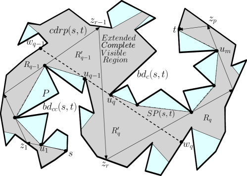
Figure 10: Every $cdrp(s,t)$ lies inside $ECV(s,t)$,
the extended complete visible region of $P$.

In the case where $SP(s,t)$ had no eaves, we had computed an $mcdrp(s,t)$ based on the analysis of the formation of mirrors on $BCV(s,t)=CV(s,t)\cap bd(P)$. If $SP(s,t)$ has eaves then we need to ensure that the $cdrp(s,t)$ crosses each eave exactly once. So, we need to consider the weak visibilty region of each eave and consider its intersection with $CV(s,t)$, yielding the extended complete visibility region $ECV(s,t)$. Extend eave $u_{q-1}u_{q}$ from $u_{q-1}$ to $bd_{c}(s,u_{q})$, meeting it at a point $w_{q-1}$ (see Figure 10). Similarly, extend $u_{q-1}u_{q}$ from $u_{q}$ to $bd_{cc}(u_{q-1},t)$, meeting it at a point $w_{q}$. Since $z_{r-1}z_{r}$ intersects $u_{q-1}u_{q}$, (i) $z_{r-1}$ and $z_{r}$ must be weakly visible from $u_{q-1}u_{q}$, (ii) $z_{r-1}$ belongs to $bd_{c}(w_{q-1},u_{q})$, and (iii) $z_{r}$ belongs to $bd_{cc}(u_{q-1},w_{q})$. Let $R_{q-1}$ be the region of $P$ bounded by $bd_{c}(s,w_{q-1})$, $SP(s,u_{q-1})$ and $u_{q-1}w_{q-1}$. Let $R^{\prime}_{q-1}$ be the region of $P$ bounded by $bd_{c}(w_{q-1},u_{q})$, and $w_{q-1}u_{q}$. Let $R^{\prime}_{q}$ be the region of $P$ bounded by $bd_{cc}(u_{q-1},w_{q})$, and $u_{q-1}w_{q}$. Let $R_{q}$ be the region of $P$ bounded by $SP(u_{q},t)$, $u_{q}w_{q}$, and $bd_{cc}(w_{q},t)$. We define the extended complete visible region $ECV(s,t)$ as the set of points in $R_{q-1}\cup R^{\prime}_{q-1}\cup R^{\prime}_{q}\cup R_{q}$ such that (i) the left and right tangents from every point of $R_{q-1}$ to $SP(s,u_{q-1})$ lie inside $P$, (ii) the left tangent from every point $z$ of $R^{\prime}_{q-1}$ to $SP(s,u_{q-1})$ lies inside $P$, and $z$ is visible from some point of $u_{q-1}u_{q}$, (iii) the left tangent from every point $z$ of $R^{\prime}_{q}$ to $SP(u_{q},t)$ lies inside $P$, and $z$ is visible from some point of $u_{q-1}u_{q}$, or (iv) the left and right tangents from every point of $R_{q}$ to $SP(u_{q},t)$ lie inside $P$. The shaded region in Figure 10 shows $ECV(s,t)$. We have the following sequel to Lemma 4.

Lemma 13.

Every $cdrp(s,t)$ lies inside $ECV(s,t)$.

Proof.

$CV(s,t)$ is augmented to form $ECV(s,t)$ as defined earlier. This augmentation considers the weak visibility region of an eave. As per the notations of Lemma 12, the turning points $z_{1},\ldots,z_{r-2}$ and $z_{r+1},\ldots,z_{p}$ of $cdrp(s,t)$ lie in $CV(s,t)$ and hence in $ECV(s,t)$. The turning points $z_{r-1}$ and $z_{r}$ lie in the weak visibility region of the eave $u_{q-1}u_{q}$ and hence, in $ECV(s,t)$. Thus, the entire $cdrp(s,t)$ lies inside $ECV(s,t)$. ∎

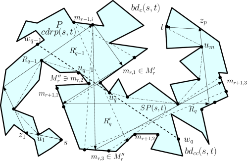
Figure 11: Starting from a mirror $m_{r-1,i}$, two mirror sets $M^{\prime}_{r}=(m_{r,1})$ and $M^{\prime\prime}_{r}=(m_{r,2},m_{r,3})$ are formed on opposite sides of the eave $u_{q-1}u_{q}$. Note that $M_{r}=M^{\prime}_{r}\cup M^{\prime\prime}_{r}=(m_{r,1},m_{r,2},m_{r,3})$.

We next proceed with the formation of mirrors on $ECV(s,t)\cap bd(P)$. Let $m_{r-1,i}$ of $M_{r-1}$ be partially or entirely on a reflecting edge of $R^{\prime}_{q-1}$, where $r-1$ is the smallest index of all mirrors on reflecting edges of $R^{\prime}_{q-1}$ (see Figure 11). Since some points of $R^{\prime}_{q}$ may become visible from $m_{r-1,i}$, the next set of mirrors $M_{r}$ consists of two subsets of mirrors $M^{\prime}_{r}$ and $M^{\prime\prime}_{r}$, where all mirrors of $M^{\prime}_{r}$ belong to reflecting edges of $R^{\prime}_{q-1}$, and all mirrors of $M^{\prime\prime}_{r}$ belong to reflecting edges of $R^{\prime}_{q}$. So, $M_{r}$ includes the union of mirror sets $M^{\prime}_{r}$ and $M^{\prime\prime}_{r}$. Observe that some mirrors of $M_{r+1}$ are created on the reflecting edges of $R^{\prime}_{q}$ due to mirrors in $M^{\prime}_{r}$, and the mirrors of $M_{r+1}$ are created on the reflecting edges of $R^{\prime}_{q}\cup R_{q}$ due to mirrors in $M^{\prime\prime}_{r}$. No mirror of $M_{r-1}$ can see any mirror of $M_{r+1}$, satisfying Lemma 7.

For computing mirror sets $M^{\prime}_{r}$ and $M^{\prime\prime}_{r}$, $M^{\prime}_{r+1}$ and $M^{\prime\prime}_{r+1},\cdots$, $M^{\prime}_{r+\alpha(r-1)}$ and $M^{\prime\prime}_{r+\alpha(r-1)}$, the process can be viewed as first computing $M^{\prime}_{r},M^{\prime}_{r+1},...,M^{\prime}_{r+\alpha(r-1)}$ on reflecting edges of $R^{\prime}_{q-1}$, and then computing $M^{\prime\prime}_{r},M^{\prime\prime}_{r+1},\cdots,M^{\prime\prime}_{r+\alpha(r-1)}$ on reflecting edges of $R^{\prime}_{q}$ from mirrors of reflecting edges of $R^{\prime}_{q-1}$. Observe that mirrors on reflecting edges of $R^{\prime}_{q-1}$ can be created from mirrors of $R^{\prime}_{q-1}$ of lower index (such as $M_{r-1,i}\in R^{\prime}_{q-1}$), or from mirrors of $bd_{c}(s,w_{q-1})$. So, the two types of mirrors on reflecting edges of $R^{\prime}_{q-1}$ can be constructed by scanning $bd_{c}(w_{q-1},u_{q})$ twice. Computing mirrors of $M^{\prime\prime}_{r},M^{\prime\prime}_{r+1},\cdots$ can be done by scanning $bd_{cc}(u_{q-1},w_{q})$ once.

For computing mirrors sets as mentioned above, we require to compute weakly visible regions from edges of $ECV(s,t)$. Shortest path trees rooted at vertices of $ECV(s,t)$ are computed following $bd_{c}(s,u_{q})$ using the method by Hershberger [12] as stated earlier. After computing $SPT(u_{q})$, $SPT(u_{q-1})$ is computed treating the eave $u_{q-1}u_{q}$ as the next edge. Subsequently, shortest path trees are computed following $bd_{cc}(u_{q-1},t)$. The process of computing sets of mirrors $M_{r+1},M_{r+2},\ldots,M_{k}$ continues as before, until $t$ becomes visible from some mirror of $M_{k}$. Therefore, the total number of mirrors created is clearly $O(n(n+\beta))$, as in Lemma 10. Finally, an $mcdrp(s,t)$ is computed as described in Section 3.1.3. We now summarize the result for polygons with one eave in the following lemma.

Lemma 14.

If $SP(s,t)$ has an eave $u_{q-1}u_{q}$, then an $mcdrp(s,t)$ can be computed in $O(n(n+\beta))$ time.

For the case of $SP(s,t)$ having two or more eaves, mirrors can be computed between every two consecutive eaves and across every eave, as explained earlier until $t$ becomes visible from a mirror of $M_{k}$. We have the following lemma.

Lemma 15.

If $SP(s,t)$ has two or more eaves, then an $mcdrp(s,t)$ can be computed in $O(n(n+\beta))$ time.

The major steps of the algorithm are stated as follows.

Input: A source $s$ and a destination $t$ inside an $n$-vertex simple polygon $P$

Output: $mcdrp(s,t)$, if it exists

Compute the Euclidean shortest path $SP(s,t)$ from $s$ to $t$;

Compute the extended complete visibility region $ECV(s,t)$ of $P$;

Starting from $s$, compute mirrors of $M_{1},M_{2},\ldots,M_{k}$ until $t$ becomes visible from some mirror of $M_{k}$;

Starting from $t$, compute $cdrp(t,s)=(t,z_{k},\ldots,z_{2},z_{1},s)$ by locating turning points on mirrors of $M_{k},M_{k-1},\ldots,M_{1}$;

Output $cdrp(s,t)$ as the $mcdrp(s,t)$;

Algorithm 1 Computing $mcdrp(s,t)$

We conclude the computation of the $mcdrp(s,t)$ with the following theorem.

Theorem 16.

For a source point $s$ and a destination point $t$ inside an $n$-vertex simple polygon $P$, an $mcdrp(s,t)$ can be computed in $O(n(n+\beta))$ time if a $cdrp(s,t)$ exists.

Proof.

First of all note that, the specific way in which we construct mirrors as discussed in Section 3.1.2 ensures that (a) the path is a simple path, crossing $SP(s,t)$ at each of its eaves exactly once, and (b) we can always find a $cdrp(s,t)$, if one exists. The cost of computing the mirrors in $M_{1},M_{2},\cdots,M_{k}$ is $O(n(n+\beta))$ as shown in Lemmas 10, 11, 14 and 15. The computed $cdrp(s,t)$ is actually also an $mcdrp(s,t)$ as its turning points are chosen on mirrors from mirror sets $M_{i}$ with minimum index $i$ on the reflecting edges, as mentioned and required in Corollary 8.

∎

4 Exploring the relationship between $cdrp(s,t)$ and $drp(s,t)$

In this section, we establish two properties relating (minimum) $cdrp(s,t)$ and (mimimum) $drp(s,t)$. The first one deals with an approximation ratio and the second one deals with a diameter.

4.1 Comparing the number of turns between an $mcdrp(s,t)$ and an optimal $drp(s,t)$

Though not the main focus of our work, we explore the relation of an $mcdrp(s,t)$ with the optimal $drp(s,t)$ and the $mlp(s,t)$. We first consider the case where $SP(s,t)$ has no eaves.

Lemma 17.

If $SP(s,t)$ does not have an eave, then the number of turns in an $mcdrp(s,t)$ is at most twice that of an optimal $drp(s,t)$.

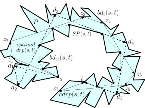
Figure 12: There may be two turning points in a $mcdrp(s,t)$ corresponding to every turning point of an optimal $drp(s,t)$.

Proof.

Let $d_{i}\in bd_{c}(s,t)$ be a turning point of an optimal $drp(s,t)$ (see Figure 12). Traverse this optimal path from $d_{i}$ to $t$ until a turning point $d_{j}\in bd_{c}(d_{i},t)$ is reached. If $d_{i}d_{j}$ is a segment and it does not intersect the $mcdrp(s,t)$, then there is no turning point of this $mcdrp(s,t)$ on $bd_{c}(s,t)$ between $d_{i}$ and $d_{j}$. If $d_{i}d_{j}$ is a segment and it intersects the $mcdrp(s,t)$, then there cannot be three or more turning points of $mcdrp(s,t)$ on $bd_{c}(d_{i},d_{j})$ due to Lemma 7, because in such a case the first and the third turning points would become visible. If $d_{i}d_{j}$ is not a segment, then no turning point of the optimal $drp(s,t)$ between $d_{i}$ and $d_{j}$ belongs to $bd_{c}(d_{i},d_{j})$. Then, this path between $d_{i}$ and $d_{j}$ still intersects the $mcdrp(s,t)$ exactly twice, and there can be at most two turning points of the $mcdrp(s,t)$ on $bd_{c}(d_{i},d_{j})$. In the worst case, all turning points of the optimal $drp(s,t)$ lie on $bd_{c}(s,t)$, and every link of this path intersects the $mcdrp(s,t)$ twice, and therefore, the number of turns in the $mcdrp(s,t)$ is at most twice that of the optimal $drp(s,t)$. ∎

Lemma 18.

If $SP(s,t)$ does not have an eave, then the number of links in an $mcdrp(s,t)$ is at most one less than twice the number of links in an $mlp(s,t)$.

Proof.

Consider the maximal chord $ab$ of any link of an $mlp(s,t)$, where $a,b\in bd(P)$ and $a\in bd_{c}(s,b)$. Due to Lemma 7, there can be at most two turns of an $mcdrp(s,t)$ in $bd_{c}(a,b)$. For the first and the last link of $mlp(s,t)$, there can be at most one link each, in an $mcdrp(s,t)$. So, the number of links in an $mcdrp(s,t)$ is at most one less than twice the number of links in an $mlp(s,t)$. ∎

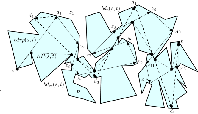
Figure 13: An optimal $drp(s,t)$ uses extensions of every eave of $SP(s,t)$ as its links. For every turn of the optimal $drp(s,t)$ after initial two turns, there are four turns of the $cdrp(s,t)$. Observe that the $cdrp(s,t)$ is also $mcdrp(s,t)$.

We now generalize these results for any simple polygon $P$.

Theorem 19.

For any simple polygon $P$, the number of turns in any $mcdrp(s,t)$ is at most $c\cdot opt$, where $2\leqslant c\leqslant 4$. Here $opt$ denotes the number of turns in an optimal $drp(s,t)$. Moreover, the number of links in any $mcdrp(s,t)$ is at most $2((|mlp(s,t)|+l)-1)\leqslant 4|mlp(s,t)|-1$, where $|mlp(s,t)|$ is the number of links in an $mlp(s,t)$ and $l\leqslant|mlp(s,t)|$ is the number of eaves in $SP(s,t)$.

Proof.

Let us count the number of turns $k$ taken by the $cdrp(s,t)$ computed by our algorithm (Algorithm 1). Recall the definition of $R_{q-1},R^{\prime}_{q-1},R^{\prime}_{q},R_{q}$ as in Figure 11. We know from Lemma 17 that there can be two turns in $R_{q-1}$ of the $cdrp(s,t)$ for every turn of an optimal $drp(s,t)$. The same argument holds for turning points in $R_{q}$. If we assume that an optimal $drp(s,t)$ uses $w_{q-1}w_{q}$ as a link in its path from $s$ to $t$, then the $cdrp(s,t)$ can have two turning points in $R^{\prime}_{q-1}$ and two more turning points in $R_{q}$. So, $k\leqslant 2opt+2$ for one eave. If $SP(s,t)$ has $l$ eaves and an optimal $drp(s,t)$ uses extensions of every eave (see Figure 13), then $k\leqslant 2opt+2l$. Since $opt\geqslant l$, $k\leqslant c\cdot opt$, where $2\leqslant c\leqslant 4$.

Using Lemma 18, and considering the fact that at most two additional turns can be introduced near each eave in an $mcdrp(s,t)$, it follows that the number of links in an $mcdrp(s,t)$ is at most $2(|mlp(s,t)|+l)-1)\leqslant 4|mlp(s,t)|-1$. ∎

Let us discuss how to cross-check the upper bound of $c$ for the $mcdrp(s,t)$ computed by our algorithm. It can be seen that counting the number of additional turns actually taken by our computed $mcdrp(s,t)$ at each eave, a realistic tighter upper bound for $c$ can be estimated using Theorem 19. Moreover, the number of turns in an optimal $drp(s,t)$ is at least the number of turns of a $mlp(s,t)$. Since an $mlp(s,t)$ can be computed in linear time [9, 10], the entire checking procedure can also be done in linear time.

In the worst case, the approximation ratio $c$ may be 4, and therefore worse than the result in [11]. Both the approximation algorithms can be run and the one giving the minimum number of turns can be taken as the final result. However, it is interesting to observe that the $mcdrp(s,t)$ computed by our algorithm measures within a small constant factor of the optimal $drp(s,t)$.

4.2 Constrained diffuse reflection diameter

Let $a$ and $b$ be two vertices of $P$ such that the number of turns in an optimal $drp(a,b)$ is maximum amongst all pairs of vertices of $P$. The number of turning points in such a path is called the diffuse reflection diameter of $P$. The relationship between the diffuse reflection diameter of $P$ and the number of vertices $n$ of $P$ has been studied in [4, 13]. Here we establish a similar relationship for constrained diffuse reflection paths in $P$.

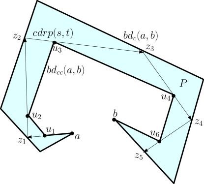
Figure 14: All edges of $bd_{c}(a,b)$ except the first one can have turning points of a $mcdrp(a,b)$.

Theorem 20.

If there exists a $cdrp(a,b)$ in $P$, then the number of turns in $mcdrp(a,b)<\frac{n}{2}$.

Proof.

Let $P$ be a spiral polygon of $n$ vertices (see Figure 14). Let $a$ and $b$ be two vertices of $P$ such that all vertices of $bd_{c}(a,b)$ are convex and all vertices of $bd_{cc}(a,b)$ are reflex. Since the diameter in $P$ is between $a$ and $b$, there always exists a $cdrp(a,b)$ in $P$, with all turning points on $bd_{c}(a,b)$. Observe that every edge of $bd_{c}(a,b)$ except the edge incident on $a$ can have a turning point of $mcdrp(a,b)$. Since the non-consecutive turning points of the $mcdrp(a,b)$ are not mutually visible due to Lemma 7, and their visibility can only be blocked by $bd_{cc}(a,b)$, the number of edges of $bd_{cc}(a,b)$ must be at least one more than the number of turns of $mcdrp(a,b)$. So, the bound holds for any spiral polygon $P$ and it is tight. This scenario is the worst-case for any simply polygon $P$, where $SP(a,b)$ has no eaves.

Assume that $SP(a,b)$ has one eave $u_{q-1}u_{q}$. Cut $P$ into two sub-polygons using $u_{q-1}u_{q}$. Since the bound for spiral polygons holds for each of these two sub-polygons, the bound also holds for $P$. If $SP(s,t)$ has two or more eaves, then $P$ can be cut using each eave, and the bound holds for the entire polygon $P$. ∎

Barequet et al. [4] have proved an upper bound of $\lfloor{\frac{n}{2}}\rfloor-1$ on the diffuse reflection diameter of $P$. Though a $drp(a,b)$ exists for any pair of points $a$ and $b$ in $P$, no $cdrp(a,b)$ may exist. Theorem 20 ensures that as long as a $cdrp(a,b)$ exists, the number of reflections in $mcdrp(a,b)$ has a similar worst-case upper bound of $\frac{n}{2}$. This bound is significant because such an $mcdrp(a,b)$ may have more turning points than an optimal $drp(a,b)$.

5 Concluding remarks

Our algorithm for computing an $mcdrp(s,t)$ in a simple polygon can be viewed as a transformation of $SP(s,t)$ and $mlp(s,t)$ to $mcdrp(s,t)$. It will be interesting to see whether an $mcdrp(s,t)$ can also be computed in a polygon with holes using similar transformations. In such a scenario, observe that the region enclosed by $SP(s,t)$ and an $mcdrp(s,t)$ may contain holes, making the problem difficult.

References

- [1] B. Aronov, A. Davis, T. Dey, S. P. Pal, and D. Prasad. Visibility with multiple reflections. Discrete & Computational Geometry, 20:61–78, 1998.
- [2] B. Aronov, A. Davis, T. Dey, S. P. Pal, and D. Prasad. Visibility with one reflection. Discrete & Computational Geometry, 19:553–574, 1998.
- [3] B. Aronov, A. R. Davis, J. Iacono, and A. S. C. Yu. The complexity of diffuse reflections in a simple polygon. In Proceedings of the 7th Latin American Symposium on Theoretical Informatics, Lecture Notes in Computer Science, volume 3887, pages 93–104. Springer, Germany, 2006.
- [4] G. Barequet, S. Cannon, E. Fox-Epstein, B. Hescott, D. L. Souvaine, C. D. Tóth, and A. Winslow. Diffuse reflections in simple polygons. CoRR, abs/1302.2271, 2013.
- [5] V. Chandru, S. K. Ghosh, A. Maheshwari, V. T. Rajan, and S. Saluja. NC-algorithms for minimum link path and related problems. Journal of Algorithms, 19:173–203, 1995.
- [6] A. R. Davis. Visibility with Reflection in Triangulated Surfaces. PhD thesis, Polytechnic University, USA, 1998.
- [7] M. de Berg. Ray Shooting, Depth Orders and Hidden Surface Removal. Lecture Notes in Computer Science, vol. 703. Springer-Verlag, Berlin, Germany, 1993.
- [8] J. Foley, A. van Dam, S. Feiner, J. Hughes, and R. Phillips. Introduction to computer graphics. Addison-Wesley, Reading, MA, 1994.
- [9] S. K. Ghosh. Computing visibility polygon from a convex set and related problems. Journal of Algorithms, 12:75–95, 1991.
- [10] S. K. Ghosh. Visibility Algorithms in the Plane. Cambridge University Press, Cambridge, UK, 2007.
- [11] S. K. Ghosh, P. P. Goswami, A. Maheshwari, S. C. Nandy, S. P. Pal, and S. Sarvattomamda. Algorithms for computing diffuse reflection paths in polygons. The Visual Computer, 28(12):1229–1237, 2012.
- [12] J. Hershberger. Finding the visibility graph of a polygon in time proportional to its size. Algorithmica, 4:141–155, 1989.
- [13] Arindam Khan, Sudebkumar Prasant Pal, Mridul Aanjaneya, Arijit Bishnu, and Subhas C. Nandy. Diffuse reflection diameter and radius for convex-quadrilateralizable polygons. Discrete Applied Mathematics, 161(10-11):1496–1505, 2013.
- [14] D. T. Lee and F. P. Preparata. Euclidean shortest paths in the presence of rectilinear barriers. Networks, 14:393–415, 1984.
- [15] S. P. Pal, S. Brahma, and D. Sarkar. A linear worst-case lower bound on the number of holes in regions visible due to multiple diffuse reflections. Journal of Geometry, 81:5–14, 2004.
- [16] D. Prasad, S. P. Pal, and T. Dey. Visibility with multiple diffuse reflections. Computational Geometry: Theory and Applications, 10:187–196, 1998.
- [17] S. Suri. A linear time algorithm for minimum link paths inside a simple polygon. Computer Graphics, Vision, and Image Processing, 35:99–110, 1986.