Blue straggler evolution caught in the act in the Large Magellanic Cloud globular cluster Hodge 11

Abstract

High-resolution Hubble Space Telescope imaging observations show that the radial distribution of the field-decontaminated sample of 162 ‘blue straggler’ stars (BSs) in the $11.7^{+0.2}_{-0.1}$ Gyr-old Large Magellanic Cloud cluster Hodge 11 exhibits a clear bimodality. In combination with their distinct loci in color–magnitude space, this offers new evidence in support of theoretical expectations that suggest different BS formation channels as a function of stellar density. In the cluster’s color–magnitude diagram, the BSs in the inner 15^′′ (roughly corresponding to the cluster’s core radius) are located more closely to the theoretical sequence resulting from stellar collisions, while those in the periphery (at radii between 85^′′ and 100^′′) are preferentially found in the region expected to contain objects formed through binary mass transfer or coalescence. In addition, the objects’ distribution in color–magntiude space provides us with the rare opportunity in an extragalactic environment to quantify the evolution of the cluster’s collisionally induced BS population and the likely period that has elapsed since their formation epoch, which we estimate to have occurred $\sim$4–5 Gyr ago.

1 Introduction

In globular cluster (GC) color–magnitude diagrams (CMDs), single stars that are more massive than the stars located at the main-sequence turn-off (MSTO) are expected to evolve off the MS. If all member stars in a GC were to evolve in isolation and without undergoing any dynamical interactions, the MS locus beyond the MSTO should be unoccupied. In reality, however, blue straggler stars (BSs)—which are more massive than stars at the MSTO—nevertheless occupy the bright MS extension (e.g., Sandage, 1953; Stryker, 1993). Two scenarios for BS formation have been suggested, involving either mass transfer between or coalescence of close binary companions (e.g., McCrea, 1964; Zinn & Searle, 1976; Carney et al., 2001; Tian et al., 2006; Lu et al., 2010, 2011), or direct stellar collisions (e.g., Hills et al., 1976; Lombardi et al., 2002; Lu et al., 2010, 2011).

The relative importance of these formation channels is still unclear. Knigge et al. (2009) found a strong correlation between the number of BSs in Galactic GC (GGC) cores and the associated core mass, but only a weak correlation with the predicted number of BSs formed through collisions; such a correlation may only be seen for extremely dense GGCs, however. Similarly, Piotto et al. (2004) did not find any significant correlation between the global BS frequency and the collision rate in their sample clusters. However, they found that the BS luminosity function is noticeably different in clusters brighter and fainter than $M_{V}=-8.8$ mag (for theoretical arguments, see Davies et al., 2004). Simulations indicate that the relative importance of both formation scenarios varies as a cluster evolves (Hypki & Giersz, 2013).

Ferraro et al. (2012) suggest that the radial profile of the relative BS frequency—the number of BSs normalized to that of horizontal-branch (HB) or red-giant-branch (RGB) stars—may be a good tracer to quantify a cluster’s dynamical age. In dynamically young GCs, where the relative BS frequency is roughly flat, e.g., $\omega$ Cen, Palomar 14, and NGC 2419 (Ferraro et al., 2012), BSs formed through mass transfer dominate (e.g., Mapelli et al., 2006; Hypki & Giersz, 2013). On the other hand, in GCs of intermediate dynamical age the BS frequency’s radial profile displays a ‘bimodality’ (Ferraro et al., 1997, 2012; Mapelli et al., 2006; Hypki & Giersz, 2013). Stellar collisions dominate the central, crowded region, while mass transfer dominates the clusters’ outer regions (e.g., 47 Tucanae, M3, and NGC 6752; Mapelli et al. 2006). In addition, BSs in dynamically old GCs (e.g., M30, M75, M79, and M80; Ferraro et al. 2012) exhibit even clearer signatures of collisional formation. Ferraro et al. (2009) discovered two distinct BS sequences in the CMD of M30, which trace the theoretical single-age stellar-collision and mass-transfer tracks. Sills et al. (2002) showed that collision products are not chemically homogeneous, so that collisionally formed BSs will be redder and fainter than their fully chemically mixed counterparts (Bailyn & Pinsonneault, 1995). This is consistent with the results of Ferraro et al. (2009).

One may thus expect for both (dynamically) intermediate-age and old GCs that the number of BSs formed through either channel should be comparable. In the absence of any clear substructures, collisionally induced BSs are expected to be preferentially located in a GC’s inner regions compared with BSs formed through mass transfer. Given the prediction that BSs of different origins will occupy different parts of color–magnitude space, the distribution of the different BS types in the CMD will depend on their radial distance from the cluster center (Ferraro et al., 2009). However, since the BSs in a given GC are not expected to all form simultaneously, the theoretically expected single-age BS sequences will be broadened (cf. Tian et al., 2006; Lu et al., 2010, 2011), and both BS types may partially overlap in color–magnitude space. However, provided that both populations are not fully mixed, a robust detection of two subgroups in the CMD should still be possible.

Studies of extragalactic BSs are relatively rare. Shara et al. (1998) detected 42 BS candidates in the Small Magellanic Cloud cluster NGC 121 and confirmed 23 stars as genuine BSs. In the Large Magellanic Cloud (LMC) clusters NGC 1466 and NGC 2257, Johnson et al. (1999) found 73 and 67 BSs, respectively, while Mackey et al. (2006)’s analysis of the LMC cluster ESO 121-SC03 yielded 32 BSs.

Using high-resolution Hubble Space Telescope (HST) observations, here we investigate the radial dependence of the BS frequency in the LMC GC Hodge 11. We detect a significant number of BSs and a clear bimodality in the cluster’s radial BS frequency. We show that the BSs in the inner region are located more closely to the theoretical ‘collision sequence’ (bluer and fainter on average), while those in the cluster’s outskirts are preferentially found in the ‘binary region’ (redder and brighter). This result, combined with the discovery that Hodge 11 hosts one of the largest BS populations in any Galactic or extragalactic cluster known to date, offers unprecedented evidence in support of the theoretical predictions and allows us to quantify the evolution of the cluster’s collisionally formed BS population.

2 Data

Our data sets were obtained with the HST’s Wide Field and Planetary Camera-2, employing the F555W (equivalent and henceforth referred to as $V$) and F814W ($\sim I$) filters (for observational details, see de Grijs et al., 2002). The total exposure times of the observations used were 435 and 960 s in the $V$ and $I$ filters, respectively. We applied point-spread-function fitting to obtain the cluster’s stellar photometric catalog (Dolphin, 2000, 2005). The cluster center was determined as described by de Grijs et al. (2013). We also obtained the stellar catalog of a nearby field region (for observational details, see Castro et al., 2001) to statistically reduce contamination by background stars (for procedural details, see Hu et al., 2010): the results are shown in Fig. 1. The number of objects located in the BS region (see below for definition) in the original Hodge 11 CMD is 338; the decontaminated CMD contains 162 stars in the same region. This latter sample forms the basis of our analysis in this Letter. Our photometric catalog is $>95$% complete in the relevant magnitude range, even in the highest-density central region. Figure 2a displays the spatial distribution of all observed stars in the Hodge 11 area covered by our HST field of view, as well as its BS population.

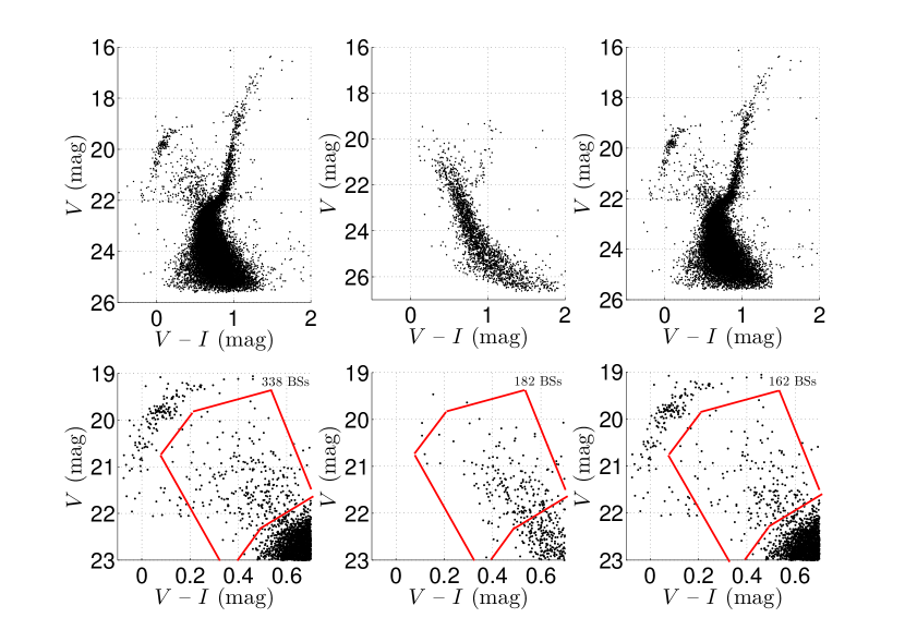
Figure 1: (top left) Original Hodge 11 CMD. (top middle) CMD of a carefully selected nearby field region (cf. Castro et al., 2001). (top right) Hodge 11 CMD after field-star decontamination. (bottom) Corresponding CMD zooms focusing on the BS-dominated region. The number of BSs and the boundaries adopted for the BS region (red outlines; see text) are also indicated. The small difference between the total number of objects in the BS region (bottom left) and the sum of the BSs identified in the bottom-middle and bottom-right panels is due to the statistical nature of our field-star decontamination procedure (cf. Hu et al., 2010).

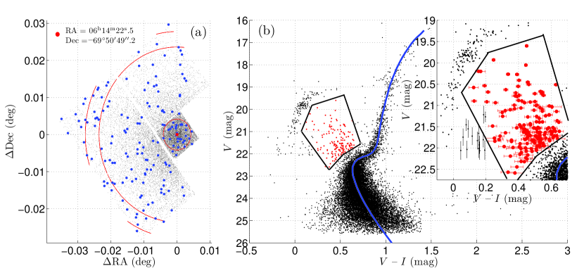
Figure 2: (left) Spatial distribution of stars observed in the Hodge 11 area. Red point: Cluster center. Blue points: BSs. Red (partial) concentric circles indicate radii of $R=15,85$, and $100^{\prime\prime}$. (right) Corresponding HST CMD, including the best-fitting Bertelli et al. (2008) isochrone (blue). Red points represent our BS selection; the inset shows the photometric uncertainties for all BS candidates. Black points with error bars have photometric errors $\Delta V>0.1$ mag (color uncertainties have been omitted for clarity). Thick solid lines delineate the BS region adopted.

We divided the MS and RGB regions in the Hodge 11 CMD into 32 bins of $\sim 0.30$ mag each between $V=18.3$ and 27.0 mag. In each magnitude range, we determined the peak and $3\sigma$ spread of the color distribution using a Gaussian function (which provided appropriate fits at any magnitude). Spectroscopic abundance determinations show that Hodge 11 is metal-poor, [Fe/H] = $-2.1\pm 0.2$ dex (Cowley et al., 1982; Olszewski et al., 1991) to $-1.86$ dex (Grocholski et al., 2006). Adopting a metallicity $Z=0.0002$ ([Fe/H] $\approx-1.98$ dex) and using the ridgeline thus obtained, we determined the best-fitting isochrone based on the Padova stellar evolutionary models (Bressan et al., 2012) and calculated the MSTO locus. We thus determined a cluster age of $\log(t\mbox{ yr}^{-1})=10.07\pm 0.01$ ($11.7^{+0.2}_{-0.1}$ Gyr; cf. Johnson et al., 1999) and an extinction of $E(B-V)=0.09\pm 0.01$ mag. The latter is in excellent agreement with Walker (1993)’s determination of $E(B-V)=0.08\pm 0.02$ mag. We adopted the canonical LMC distance modulus, $(m-M)_{0}=18.50$ mag, so that $1^{\prime\prime}\equiv 0.24$ pc.

Many of the cluster’s HB stars are located in the extreme blue HB (EHB). Our sample BSs can easily be distinguished from these (E)HB stars by adopting a minimum (E)HB–BS difference in color and magnitude of 0.3 mag. Our selection is robust, since the (E)HB stars and BSs are clearly separated in the CMD (see Fig. 2) and the absolute photometric errors are $\ll 0.3$ mag.

Finally, we identify a star as a likely BS if it meets all of the following criteria:

1. It is bluer and brighter than the single-star MSTO locus.

2. Its distance in color–magnitude space from the MSTO and MS ridgeline is $>3\sigma$ ($\sigma$ refers to the intrinsic spread in MS color at the magnitude of interest).

3. Its photometric uncertainty is $<0.1$ mag in both filters.

Figure 2b shows the Hodge 11 HST CMD, where the inset focuses on the region typically populated by BSs. The red points represent our (field-decontaminated) BS candidates. The small black points with error bars are objects whose photometric errors are $>0.1$ mag, while most of the error bars of the red points are smaller than the symbol size. Inspection on the original images of the sources with large error bars revealed that they either are affected by instrumental artefacts (including low signal-to-noise ratios or closely juxtaposed to bad pixels) or may be unresolved blends. We thus discarded these objects from our BS sample.

3 Analysis and results

Figures 3a and 3b show the cluster’s stellar number density as a function of radius for all stars with $V\leq 25$ mag. Based on the catalog of the nearby field region, we calculated the field’s average density value. We adopted the distance where the cluster’s monotonically decreasing number-density profile reaches the average field level, $R=102.3^{+2.7}_{-2.3}$ arcsec, as the cluster region.

In addition to our BS sample, we selected a sample containing RGB stars covering the magnitude range from $V=19.60$ to 22.05 mag. We normalized the number of BSs to the number of RGB stars: $f_{\rm BSs}=N_{\rm BSs}/N_{\rm RGB}$, where $N_{\rm BSs}$ and $N_{\rm RGB}$ represent the number of BSs and RGB stars, respectively. Previous studies (e.g., Ferraro et al., 2003) normalized the number of BSs to either or both HB or/and RGB stars. We adopted RGB stars as reference for reasons of consistency with previous analyses. We subsequently determined the radial dependence of the BS fraction, $f_{\rm BSs}(R)$: see Fig. 3c. Normalization of the BS number to the number of HB stars results in a similar, although somewhat flatter trend. This BS-fraction profile is very similar to the equivalent radial dependences in 47 Tuc, M3, and NGC 6752 (Mapelli et al., 2006).

The number of BSs in Hodge 11 is extremely large. Ferraro et al. (2007) summarized the number of BSs detected in 26 GGCs, ranging from four (NGC 5024) to 137 (NGC 5272). In Hodge 11, we detected 150 BSs within $R=100^{\prime\prime}$; the total number of BSs on all four chips of our Hodge 11 observations reaches 162 (see Section 4 for an assessment of the level of completeness of our observations’ areal coverage). Since the BS distribution associated with Hodge 11 is very extended, the number of BSs located in our outer subsample, $R\in[85^{\prime\prime},100^{\prime\prime}]$, is significant. This annulus contains 27 BSs, and hence this large number of BSs strengthens the statistical reliability of our conclusions.

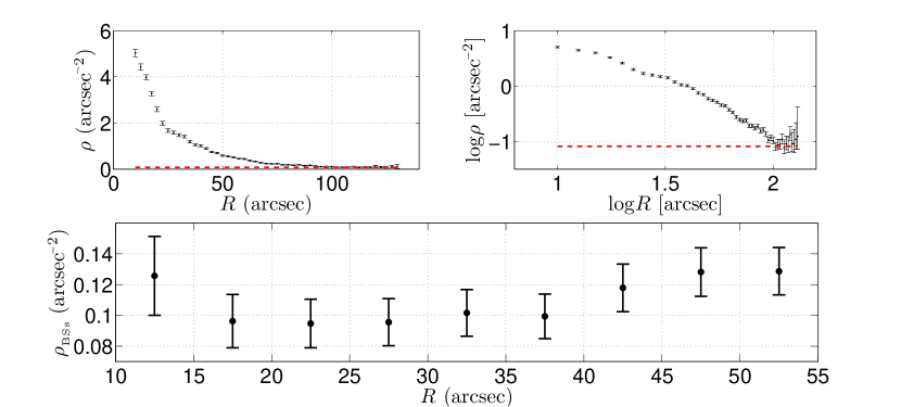
Figure 3: (a) Hodge 11 number-density profile (corrected for partial areal coverage). The red dashed line indicates the average field density, implying a cluster size of $R=102.3^{+2.7}_{-2.3}$ arcsec. (b) Corresponding logarithmic number-density profile. (c) BS-fraction profile (normalized to the number of RGB stars) of Hodge 11, including Poissonian uncertainties.

Mackey & Gilmore (2003) determined a cluster core radius of $R_{\rm core}=12.14\pm 0.66$ arcsec. Our number-density profile exhibits a relatively sharp radial decline to $R\sim 15$–$20^{\prime\prime}$. Therefore, we defined an inner BS subsample covering the cluster core at $R\leq 15^{\prime\prime}$ (Fig. 4, left). The red and blue points in the CMD of Fig. 4 (left) represent the inner ($R\leq 15^{\prime\prime}$) and outer ($R\in[85^{\prime\prime},100^{\prime\prime}]$) subsamples. Both contain 27 BSs. A distinct difference is seen between the mean loci of both samples in color–magnitude space. We also show the separation between the two BS subpopulations in M30 found by (Ferraro et al., 2009, dashed line). These authors suggested that BSs below this ‘critical’ line might preferentially result from stellar collisions in relatively high-density regions, while BSs above the line are predominantly thought to have formed through mass transfer between binary companions in lower-density areas.

Considering that M30 and Hodge 11 may have different evolutionary histories and environments, using the M30 critical line to analyze the color–magnitude distribution of the Hodge 11 BSs may not be appropriate. If we shift the zero-age main sequence (ZAMS) upward in the CMD by 0.75 mag—which represents the ZAMS of equal-mass binary systems (B-ZAMS)—we see that this provides an excellent separation between both subsamples. Hence, our results for Hodge 11 support the claims of Ferraro et al. (2009) for M30: Only one outer-sample BS is unambiguously located in the ‘bottom region’ (labeled ‘A’ in Fig. 4, middle), while the 26 remaining outer-sample BSs are all located above the B-ZAMS (modulo the photometric uncertainties). In contrast, for our $R\leq 15^{\prime\prime}$ inner-sample BS selection, only four BSs are unambiguously located in this CMD region, given the photometric errors.

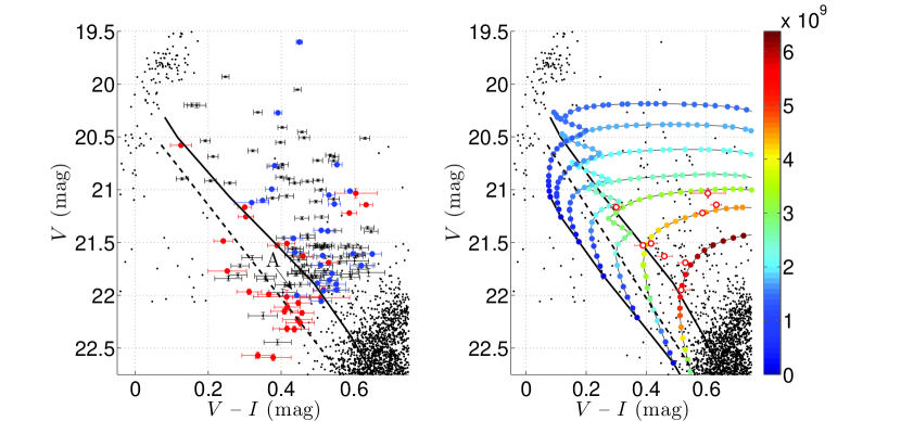
Figure 4: (left) Color–magnitude distribution of BSs in Hodge 11. Red points: BSs at $R\leq 15^{\prime\prime}$; blue points: BSs at $R\in[85^{\prime\prime},100^{\prime\prime}]$. The black dashed line indicates approximately the critical line separating the two BS sequences in M30 (Ferraro et al., 2009); the black solid line indicates the predicted ZAMS adjusted by $-0.75$ mag. (right) Evolutionary tracks of stars with masses from 1.0 to $1.6M_{\odot}$ in steps of $0.1M_{\odot}$ (bottom to top; Bertelli et al. 2008) for $Z=0.0004$ (closest available metallicity). Different colors indicate the evolutionary timescales for stars to evolve from the ZAMS to their current positions, in units of $10^{9}$ yr. Red open circles: Inner-sample BSs ($R\leq 15^{\prime\prime}$) located above the B-ZAMS.

4 Discussion

Since the cluster’s central region is very crowded, the BSs in this region are most likely preferentially the result of stellar collisions. On the other hand, since the low number density at large radii renders a high frequency of direct stellar collisions unlikely, the BSs in the cluster’s periphery most likely originate from mass transfer between the individual members in binary systems. Based on the B-ZAMS adopted, the mixture of the two BSs subsamples in the CMD seems ‘unbalanced:’ only few outer-sample BSs are found in the bottom region, while inner-sample BSs frequently ‘pollute’ the top region. We suggest three possible explanations for this observation:

1. The spatial distribution of the BSs in Hodge 11 is a two-dimensional projection of a 3D spatial distribution. Some apparent inner-sample BSs may not be genuine inner-sample members, but could be outer-sample BSs that are projected close to the cluster center. On the other hand, outer-sample BSs must always be located truly far away from the center. Geometry considerations, assuming a uniform BS distribution in the outer annulus, $R\in[85^{\prime\prime},100^{\prime\prime}]$, suggest that $4\pm 2$ (Poissonian uncertainty) outer-sample BS may be projected along the full line of sight through the cluster onto radii $R\leq 15^{\prime\prime}$.

2. BSs evolve and trace paths in the CMD. Without any new dynamical interactions, the BSs in the bottom region will move upward, but the BSs in the top area will never move downward. To estimate the approximate time necessary for BSs to evolve from the ZAMS to the region above the B-ZAMS, in Fig. 4 (right) we show evolutionary tracks from Bertelli et al. (2008) for stars of different masses. Below, we select those inner-sample BSs that are located above the B-ZAMS (red open circles) and compare their loci to the tracks for stars with masses from 1.0 to $1.6M_{\odot}$ (bottom to top; $1.6M_{\odot}$ is approximately $2M_{\rm MSTO}$). Different colors indicate different evolutionary timescales for stars to evolve from the ZAMS to their current positions.

3. There may still be some primordial binaries in the inner region, which may merge to form BSs. Once formed, they will be located in the top region.

One outer-sample BS, object ‘A’ in Fig. 4 (middle), is found in the CMD’s bottom region. Its locus cannot have been caused by the expected evolutionary color spread. This star could either be a projected foreground star or a collisionally formed cluster BS that may have been ejected dynamically to the cluster’s periphery (cf. Sigurdsson et al., 1994). Such ejected BSs will subsequently sink to the center again through the effects of two-body relaxation (dynamical mass segregation). Compared with the other cluster BSs, this star is relatively faint (and hence of relatively low mass), so that this relaxation process is likely still underway.

Accounting for scenarios 1–3 above, the radial distance bias of BSs in the Hodge 11 CMD is nevertheless significant, which suggests that our result is robust. In addition, compared with M30, the number of field BSs detected in the Hodge 11 field at radii beyond the cluster’s outer radius is very large. We identified 12 BSs in the partially observed annulus $R\in[100^{\prime\prime},130^{\prime\prime}]$, whose HST-based coverage is only 9.3% complete (for comparison, our coverage of the actual cluster area, $R\leq 100^{\prime\prime}$, is 50.2% complete). Nevertheless, if we adopt an outer boundary to the outer-sample BS population such that all observed BSs are included and compare their color–magnitude distribution with that of the inner-sample BSs, the distinction between the two samples remains significant.

If we treat all selected objects as genuine cluster BSs, the locus of the most massive BS—which should originally have been located in the ‘bottom region’ of the CMD but is found above the B-ZAMS—may have been caused by stellar evolution. Geometry considerations imply that $4\pm 2$ stars may be seen in projection, although nine inner-sample BSs that may have crossed the B-ZAMS are actually detected. This means that $5\pm 2$ objects could be evolved BSs. If correct, this allows us to estimate their time of birth at 4–5 Gyr ago. The BSs characterized by magnitudes between $V=21.0$ and 21.5 mag are probably also evolved stars. For BSs fainter than $V=21.5$ mag, the time required to evolve to their current loci is so long that their positions in the CMD may be owing to 2D projection of the cluster’s 3D spatial distribution.

5 Conclusion

Based on the predictions of stellar evolutionary models, BSs resulting from direct stellar collisions and from mass transfer between binary companions will be located along two distinct sequences. However, two well-separated sequences can only be observed if all BS formation in a given cluster occurred recently or if all BSs are short-lived. Long-term, continuous BS formation will render the expected boundary less distinct. Nevertheless, it is expected that BSs formed through either of these two mechanisms show the signature of a clustercentric radial dependence in their color–magnitude distribution. We analyzed the HST CMD of the GC Hodge 11, where we found a clear signature of such a spatial bias. The average BS in the inner region is relatively faint, while BSs in the outer region are brighter. Even when considering the possible effects of projection and evolution, this difference is robust. Our result hence offers strong evidence in support of the theoretical expectation of dual-mode BS formation and allowed us to quantify their evolutionary timescales.

References

- Bailyn & Pinsonneault (1995) Bailyn, C. D., & Pinsonneault, M. H. 1995, ApJ, 439, 705
- Carney et al. (2001) Carney, B. W., Latham, D. W., Laird, J. B., Grant, C. E., & Morse, J. A. 2001, AJ, 122, 3419
- Castro et al. (2001) Castro, R., Santiago, B. X., Gilmore, G. F., Beaulieu, S., & Johnson, R. A. 2001, MNRAS, 326, 333
- Cowley et al. (1982) Cowley, A., & Hartwick, F. F. A. 1982, ApJ, 438, 724
- Bertelli et al. (2008) Bertelli, G., Girardi, L., Marigo, P., & Nasi, E. 2008, A&A, 484, 815
-
Bressan et al. (2012)
Bressan, A., Marigo, P.,
Girardi, L., et al. 2012, MNRAS, 427, 127
(http://stev.oapd.inaf.it/cmd) - Dalessandro et al. (2008) Dalessandro, E., Lanzoni, B., Ferraro, F. R., et al. 2008, ApJ, 681, 311
- Davies et al. (2004) Davies, M. B., Piotto, G. & de Angeli, F. 2004, MNRAS, 348, 129
- de Grijs et al. (2002) de Grijs, R., Johnson, R. A., Gilmore, G. F., & Frayn, C. M. 2002, MNRAS, 331, 228
- de Grijs et al. (2013) de Grijs, R., Li, C., Zheng, Y., Deng, L., Hu, Y., Kouwenhoven, M. B. N., & Wicker, J. E. 2013, ApJ, 765, 4
- Dolphin (2000) Dolphin A. E. 2000, PASP, 112, 1383
-
Dolphin (2005)
Dolphin A. E. 2005, HSTphot User’s
Guide, v. 1.1.7b
(http://purcell.as.arizona.edu/hstphot/) - Ferraro et al. (1997) Ferraro, F. R., Paltrinieri, B., Fusi Pecci, F., et al. 1997, A&A, 324, 915
- Ferraro et al. (2003) Ferraro, F. R., Sills, A., Rood, R. T., Paltrinieri, B., & Buonanno, R. 2003, ApJ, 588, 464
- Ferraro et al. (2006) Ferraro, F. R., Sollima, A., Rood, R. T., et al. 2006, ApJ, 638, 433
- Ferraro et al. (2007) Ferraro, F. R., Fusi Pecci, F., & Bellazzini, M. 2007, A&A, 294, 80
- Ferraro et al. (2009) Ferraro, F. R., Beccari, G., Dalessandro, E. 2009, Nature, 462, 1028
- Ferraro et al. (2012) Ferraro, F. R., Lanzoni, B., Dalessandro, E., et al. 2012, Nature, 492, 393
- Johnson et al. (1999) Johnson, J. A., Bolte M., Stetson, P. B., Hesser, J. E., & Somerville, R. S. 1999, ApJ, 527, 199
- Grocholski et al. (2006) Grocholski, A. J., Cole, A. A., Sarajedini, A., Geister, D., & Smith, V. V. 2006, AJ, 132, 1630
- Hills et al. (1976) Hills, J. G., & Day, C. A. 1976, ApJ, 17, 87
- Hu et al. (2010) Hu, Y., Deng, L., de Grijs, R., Liu, Q., & Goodwin, S. P. 2010, ApJ, 724, 649
- Hypki & Giersz (2013) Hypki, A., & Giersz, M. 2013, MNRAS, 429, 1221
- Johnson et al. (1999) Johnson, J. A., Bolte, M., Stetson, P. B., Hesser, J. E., & Somerville, R. S. 1999, ApJ, 527, 199
- Knigge et al. (2009) Knigge, C., Leigh, N., & Sills, A. 2009, Nature, 457, 288
- Lombardi et al. (2002) Lombardi, J. C., Jr, Warren, J. S., Rasio, F. A., Sills, A., & Warren, A. R. 2002, ApJ, 568, 939
- Lu et al. (2010) Lu, P., Deng, L. C., & Zhang, X. B. 2010, MNRAS, 409, 1013
- Lu et al. (2011) Lu, P., Deng, L.-C., & Zhang, X.-B. 2011, RAA, 11, 1336
- Mackey & Gilmore (2003) Mackey, A. D., & Gilmore, G. F. 2003, MNRAS, 338, 85
- Mackey & van den Bergh (2005) Mackey, A. D., & van den Bergh, S. 2005, MNRAS, 360, 631
- Mackey et al. (2006) Mackey, A. D., Payne, M.J., & Gilmore, G. F. 2006, MNRAS, 369, 921
- Mapelli et al. (2006) Mapelli, M., Sigurdsson, S., Ferraro, F. R., Colpi, M., Possenti, A., & Lanzoni, B. 2006, MNRAS, 373, 361
- Mateo (1987) Mateo, M. 1987, ApJ, 323, L41
- McCrea (1964) McCrea, W. H. 1964, MNRAS, 128, 147
- Olszewski et al. (1991) Olszewski, E. W., Schommer, R. A., Suntzeff, N. B., & Harris, H. C. 1991, AJ, 101, 515
- Piotto et al. (2004) Piotto, G., de Angeli, F., King, I. R., et al. 2004, ApJ, 604, 109
- Sandage (1953) Sandage, A. 1953, AJ, 58, 61
- Shara et al. (1998) Shara, M. M., Fall, S. M., Rich, R. M., & Zurek, D. 1998, ApJ, 508, 570
- Sigurdsson et al. (1994) Sigurdsson, S., Davies, M. B., & Bolte, M. 1994, ApJ, 431, L115
- Sills et al. (2002) Sills, A., Adams, T., Davies, M. B., & Bate, M. R. 2002, MNRAS, 332, 49
- Stryker (1993) Stryker, L. L. 1993, PASP, 105, 1081
- Tian et al. (2006) Tian, B., Deng, L., Han, Z., & Zhang, X. B. 2006, A&A, 455, 247
- Walker (1993) Walker, A. R. 1993, AJ, 106, 999
- Zinn & Searle (1976) Zinn, R., & Searle, L. 1976, ApJ, 209,734