Nonparametric Multivariate $L_{1}$-median Regression Estimation with Functional Covariates

Abstract

In this paper, a nonparametric estimator is proposed for estimating the $L_{1}$-median for multivariate conditional distribution when the covariates take values in an infinite dimensional space. The multivariate case is more appropriate to predict the components of a vector of random variables simultaneously rather than predicting each of them separately. While estimating the conditional $L_{1}$-median function using the well-known Nadarya-Waston estimator, we establish the strong consistency of this estimator as well as the asymptotic normality. We also present some simulations and provide how to built conditional confidence ellipsoids for the multivariate $L_{1}$-median regression in practice. Some numerical study in chemiometrical real data are carried out to compare the multivariate $L_{1}$-median regression with the vector of marginal median regression when the covariate $X$ is a curve as well as $X$ is a random vector.

Keywords: almost sure convergence, confidence ellipsoid, functional data, kernel estimation, small balls probability, multivariate conditional $L_{1}$-median, multivariate conditional distribution.

1 Introduction

In statistics, researchers are often interested in how a variable response $Y$ may be concomitant with an explanatory variable $X$. Studying the relationship between $Y$ given a new value of the explanatory variable $X$ is an important task in non-parametric statistics. For instance, regression function provides the mean value that takes $Y$ given $X=x$. Some other characteristics of the conditional distribution, such as conditional median, conditional quantiles, conditional mode, maybe quite interesting in practice. Furthermore, it is widely acknowledged that quantiles are more robust to outliers than regression function.

Conditional quantiles are widely studied when the explanatory variable $X$ lies within a finite dimensional space. There are many references on this topic (see Gannoun et al. (2003a)).

During the last decade, thanks to progress of computing tools, there is an increasing number of examples coming from different fields of applied sciences for which the data are curves. For instance, some random variables can be observed at several different times. This kind of variables, known as functional variables (of time for instance) in the literature, allows us to consider the data as curves. The books by Bosq (2000) and Ramsay and Silverman (2005)) propose an interesting description of the available procedures dealing with functional observations whereas Ferraty and Vieu (2006) present a completely non-parametric point of view. These functional approaches mainly rely on generalizing multivariate statistical procedures in functional spaces and have been proved to be useful in various areas such as chemiomertrics (Hastie and Mallows (1993) and Quintela-del Río and Francisco-Fernández (2011)), economy (Kneip and Utikal (2001)), climatology (Besse et al. (2000)), biology (Kirkpatrick and Heckman (1989)), Geoscience (Quintela-del Río and Francisco-Fernández (2011)) or hydrology (Chebana and Ouarda (2011)). These functional approaches are generally more appropriate than longitudinal data models or time series analysis when there are, for each curve, many measurement points (Rice (2004)).

In the univariate case (i.e. $Y\in\mathbb{R}$ and $X$ is a functional covariable), among the lot of papers dealing with the nonparametric estimation of conditional quantiles, one may cite papers by Cardot et al. (2005) which introduced univariate quantile regression with functional covariate and Ferraty et al. (2005) estimates conditional quantile by inverting the conditional cumulative distribution function. Ezzahrioui and Ould-Saïd (2008) establish the almost complete convergence and the asymptotic normality in the setting of independent and identically distributed (i.i.d.) data as well as under $\alpha$-mixing condition. Dabo-Niang and Laksaci (2012) stated the convergence in $L^{p}$-norm. In the same framework, Laksaci et al. (2009) estimated the conditional quantile nonparametrically, by adapting the $L^{1}$-norm method. Recently Quintela-del Río and Vieu (2011) have used the same approach proposed by Ferraty et al. (2005) to predict future stratospheric ozone concentrations and to estimate return levels of extreme values of tropospheric ozone.

Over the past decades, researchers have shown increasing interest in studying multivariate location parameters such as multivariate quantiles in order to find suitable analogs of univariate quantiles that used to construct descriptive statistics and robust estimations of location. In contrast to the univariate case, the order of observations $Y_{i}$ laying in $\mathbb{R}^{d}$ (with $d\geq 2$) is not total. Consequently, several quantiles-type multivariate definitions have been formulated. The pioneer paper of Haldane (1948) considered a multivariate extension of the median defined as an $M$-estimator (also called spatial or $L_{1}$-median). The reader is referred to Serfling (2002) for historical reviews and comparisons. Chaudhuri (1996) and Koltchinskii (1997) defined the geometric quantile as an extension of multivariate quantiles based on norm minimization and on the geometry of multivariate data clouds.

In contrast, relative little attention has been paid to the multivariate conditional quantiles ($Y\in\mathbb{R}^{d}$ and $X\in\mathbb{R}^{s}$) and their large sample properties. Cadre (2001) defined the conditional $L_{1}$-median and provided its uniform consistency on a compact subsets of $\mathbb{R}^{s}$. Recently, De Gooijer et al. (2006) have introduced a multivariate conditional quantile notion, which extends the definition of unconditional quantiles by Abdous and Theodorescu (1992), to predict tails from bivariate time series. Cheng and De Gooijer (2007) have generalized the notion of geometric quantiles, defined by Chaudhuri (1996), to the conditional setting. They have established a Bahadur-type linear representation of the $u$-th geometric conditional estimator as well as the asymptotic normality in the i.i.d. case.

The purpose of this paper is to add some new results to the non-parametric estimation of the conditional $L_{1}$-median when $Y$ is a random vector with values in $\mathbb{R}^{d}$ while the covariable $X$ take its values in some infinite dimensional space $\mathcal{F}$. As far as we know, this problem has not been studied in literature before and the results obtained here are believed to be novel. Moreover, our motivation for studying this type of robust estimator is due to its interest in some practical applications. Note also that, it would be better to predict all components of a vector of random variables simultaneously in order to take into account the correlation between them rather than predicting each of component separately. For instance, in EDF (French electricity company) the estimation of the minimum and the maximum of the electricity power demand represents an important research issue for both economic and security reasons. Because an underestimation of the maximum consumed quantity of electricity (especially in winter) may require importation of electricity from other European countries with high prices, while an over estimation of this maximum quantitiy may induce a negative effect on the electricity distribution network. The estimation of the minimum power demand is also an important task for the same reasons. Notice that the minimum and the maximum of the electricity power demand are strongly correlated. Thus, it is more appropriate to predict these variables simultaneously rather than predicting each of them separately. On the other hand, weather variables, like temperature curves, can play a key role to explain the minimum and the maximum of power demand. Due to its robust properties, the conditional $L_{1}$-median may be used to solve this prediction problem using a temperature curve as covariate.

The paper is organized as follows. Section 2 outlines notations and the form of the new estimator. Section 3 presents the main results concerning the asymptotic behavior of the estimator, including consistency, asymptotic normality and evaluation of the bias term. An estimation of the conditional confidence region is then deduced. Section 4 is devoted to a simulation study giving an example of the estimated confidence region. An application to chemiometrical real data is proposed in Section 5, where we compare three approaches: $L_{1}$-median regression, the vector of marginal conditional median and non-functional multivariate median to predict a random vector. The proofs of the results in Section 3 are relegated to the Appendix.

2 Notations and definitions

Let us consider a random pair $(X,Y)$ where $X$ and $Y$ are two random variables defined on the same probability space $(\Omega,\mathcal{A},\mathbb{P})$. We suppose that $Y$ is $\mathbb{R}^{d}$-valued and $X$ is a functional random variable (f.r.v.) takes its values in some infinite dimensional vector space $(\mathcal{F},d(\cdot,\cdot))$ equipped with a semi-metric $d(\cdot,\cdot)$. Let $x$ be a fixed point in $\mathcal{F}$ and $F(.|x)$ be the conditional cumulative distribution function (cond. c.d.f) of $Y$ given $X=x$. The conditional $L_{1}$-median, $\mu:{\cal F}\longrightarrow\mathbb{R}^{d}$, of $Y$ given $X=x$, is defined as the miminizer over $u$ of

$$\arg\min_{u\in\mathbb{R}^{d}}\mathbb{E}[(\|Y-u\|-\|Y\|)\;|\;X=x]=\arg\min_{u\in\mathbb{R}^{d}}\displaystyle\int(\|y-u\|-\|y\|)\;dF(y\;|\;x).$$ (1)

The general definition (1) does not assume the existence of the first order moment of $\|Y\|$. However, when $Y$ has a finite expectation, $\mu(x)$ becomes a minimizer over $u$ of $\mathbb{E}[\|Y-u\|\;|\;X=x].$ Notice that the existence and the uniqueness of $\mu(x)$ is guaranteed, for $d\geq 2,$ provided that the conditional distribution function $F(\cdot|x)$ is not supported on a single straight line (see theorem 2.17 of Kemperman (1987). Hence, uniqueness holds whenever $Y$ has an absolutely continuous conditional distribution on $\mathbb{R}^{d}$ with $d\geq 2.$

Without loss of generality, we suppose in the sequel, that $\mathbb{E}\|Y\|<\infty$. Therefore for any fixed $x\in\mathcal{F}$, the conditional $L_{1}$-median $\mu(x)$ may be viewed as a minimizer of the function $G^{x}:\mathbb{R}^{d}\longmapsto\mathbb{R}$ defined, for all $u\in\mathbb{R}^{d}$, by

$$G^{x}(u):=\mathbb{E}[\|Y-u\|\;|\;X=x],$$ (2)

which is assumed to be differentiable and uniformly bounded with respect to $u$.

We introduce now some further definitions and notations. Denote by $A^{t}$ the transpose of the matrix $A$, and let $\|A\|=\sqrt{tr(A^{t}\,A)}$ be the norm trace. Notice that for any $y\in\mathbb{R}^{d}$, the function $y\longmapsto\|y\|$ is differentiable everywhere except at $z=0_{\mathbb{R}^{d}}$, one may then define (by continuity extension) its derivative as $\mathcal{U}(y)=y/\|y\|$ when $y\neq 0$ and $\mathcal{U}(y)=0$ whenever $y=0$. For any $y\neq u$, define

$$\mathcal{M}(y,u)=(1/\|y-u\|)({\bf I}_{d}-\mathcal{U}(y-u)\mathcal{U}^{t}(y-u)),$$

where ${\bf I}_{d}$ is the $d\times d$ identity matrix. We denote by $\nabla_{u}G^{x}(u)$ the gradian of the function $G^{x}(u)$ and by $H^{x}(u)$ its Hessian functional matrix (with respect to $u$). According to Koltchinskii (1997), it is easy to see that

$$\nabla_{u}G^{x}(u)=-\mathbb{E}\left[\mathcal{U}(Y-u)\;|\;X=x\right]\quad\mbox{and}$$ (3)

$$H^{x}(u)=\mathbb{E}\left[\mathcal{M}(Y,u)\;|\;X=x\right].$$ (4)

Notice that $H^{x}(u)$ is bounded whenever $\mathbb{E}\left[\|Y-u\|^{-1}\mid X=x\right]<\infty.$ According to (1) and (3), the conditional $L_{1}$-median may be then implicitly defined as a zero with respect to $u$ of the following equation:

$$\nabla_{u}G^{x}(u)=0.$$ (5)

To build our estimator, let $(X_{i},Y_{i})_{i=1,\dots,n}$ be the statistical sample of pairs which are independent and identically distributed as $(X,Y)$. Let us denote by

$$w_{n,i}(x)=\frac{\Delta_{i}(x)}{\sum_{i=1}^{n}\Delta_{i}(x)},$$

the so-called Nadaraya-Watson weights, where $\Delta_{i}(x)=K\left(d(x,X_{i})/h\right)$, with $K$ a kernel function, $h:=h_{n}$ is a sequence of positive real numbers which decreases to zero as $n$ tends to infinity.

A kernel estimator of the function $G^{x}(u)$ is given by

$$G_{n}^{x}(u)=\sum_{i=1}^{n}w_{n,i}(x)\,\|Y_{i}-u\|=\frac{\sum_{i=1}^{n}\|Y_{i}-u\|\;\Delta_{i}(x)}{\sum_{i=1}^{n}\Delta_{i}(x)}:=\frac{G^{x}_{n,2}(u)}{G^{x}_{n,1}},$$ (6)

when the denominator is not equal to 0, where

$$G^{x}_{n,j}((j-1)u)=\frac{1}{n\mathbb{E}(\Delta_{1}(x))}\sum_{i=1}^{n}\|Y_{i}-u\|^{j-1}\Delta_{i}(x),\quad\mbox{for}\quad j=1,2\quad\mbox{with}\quad G^{x}_{n,1}(0):=G^{x}_{n,1}.$$ (7)

A kernel estimate of $\nabla_{u}G^{x}(u)$ may be defined by

$$\nabla_{u}G^{x}_{n}(u):=-\sum_{i=1}^{n}w_{n,i}(x)\;\mathcal{U}(Y_{i}-u),\quad u\in\mathbb{R}^{d}.$$ (8)

According to the statement (2), the estimator of the conditional $L_{1}$-median, $\mu_{n}(x)$, may be viewed as a minimizer over $u$ of the function $G^{x}_{n}(u)$, that is

$$\mu_{n}(x)=\arg\min_{u\in\mathbb{R}^{d}}G^{x}_{n}(u),$$ (9)

or as a zero with respect to $u$ of the equation $\nabla_{u}G^{x}_{n}(u)=0.$

Similar to the Fact $2.1.1$ in Chaudhuri (1996) and Remark $2.3$ in Cheng and De Gooijer (2007), the existence of the estimator $\mu_{n}(x)$ is guaranteed by the fact that the function $u\longmapsto\sum_{i=1}^{n}w_{n,i}(x)\|Y_{i}-u\|$ explodes to infinity as $||u||\rightarrow\infty$. On the other hand, since this function is continuous with respect to $u$, then $\mu_{n}(x)$ must be a minimizer over $u$ of $\sum_{i=1}^{n}w_{n,i}(x)\|Y_{i}-u\|$. Next comes the question of uniqueness, since $\mathbb{R}^{d}$ is equipped with the Euclidean norm that is a strictly convex Banach space for $d\geq 2$, it follows from Theorem $2.17$ of Kemperman (1987) that unless all the data points $Y_{1},\dots,Y_{n}$ fall on a straight line in $\mathbb{R}^{d}$, $\sum_{i=1}^{n}w_{n,i}(x)\|Y_{i}-u\|$ must be a strictly convex function of $u$. This guarantees the uniqueness of the minimizer $\mu_{n}(x)$ in $\mathbb{R}^{d}$, for any $d\geq 2$.

3 Main Results

3.1 Further notations and hypotheses

Let $x$ be a given point in ${\cal F}$ and $\mathcal{V}_{x}$ a neighbourhood of $x$. Denote by $\mathcal{B}(x,h)$ the ball of center $x$ and radius $h$, namely $\mathcal{B}(x,h)=\{x^{\prime}\in\mathcal{F}:d(x,x^{\prime})\leq h\}$. For $(\ell,u)\in\mathbb{R}\times\mathbb{R}^{d}$, denote by $G_{\ell}^{x^{\prime}}(u)=\mathbb{E}\left[\|Y-u\|^{\ell}\mid X=x^{\prime}\right]$, for $x^{\prime}\in\mathcal{F}$. Our hypotheses are gathered here for easy reference.

• $K$ is a nonnegative bounded kernel of class $\mathcal{C}^{1}$ over its support $[0,1]$ such that $K(1)>0.$ The derivative $K^{\prime}$ exists on $[0,1]$ and satisfy the condition $K^{\prime}(t)<0,$ for all $t\in[0,1]$ and $|\int_{0}^{1}(K^{j})^{\prime}(t)dt|<\infty$ for $j=1,2.$

• For $x\in\mathcal{F}$, there exists a deterministic nonnegative bounded function $g$ and a nonnegative real function $\phi$ tending to zero, as its argument tends to 0, such that

  • $F_{x}(h):=\mathbb{P}(X\in\mathcal{B}(x,h))=\phi(r)\cdot g(x)+o(\phi(h))$ as $h\rightarrow 0.$

  • There exists a nondecreasing bounded function $\tau_{0}$ such that, uniformly in $s\in[0,1]$,

    $\displaystyle\frac{\phi(hs)}{\phi(h)}=\tau_{0}(s)+o(1),$ as $h\downarrow 0$ and, for $j\geq 1$, $\int_{0}^{1}(K^{j}(t))^{\prime}\tau_{0}(t)dt<\infty.$

• • For $x\in\mathcal{F}$, $|G^{x}(u)-G^{x^{\prime}}(u)|\leq c_{1}d^{\beta}(x,x^{\prime})$ uniformly in $u$, for some $\beta>0$ and a constant $c_{1}>0$, whenever $x^{\prime}\in\mathcal{V}_{x}$,

  • For $x^{\prime}\in\mathcal{F}$, the Hessian matrix $H^{x^{\prime}}(u)$ is continuous in $\mathcal{V}_{x}$:

    $\sup_{x^{\prime}\in B(x,h)}\|H^{x}(u)-H^{x^{\prime}}(u)\|=o(1)$.

  • For some integer $m\geq 2$, $G_{-m}^{x}(\mu(x))<\infty$ and $G_{-m}^{x^{\prime}}(\mu(x))$ is continuous in $\mathcal{V}_{x}$.

  • For some integer $m\geq 1$ and any $(k,j)$, $1\leq k\leq d$, $1\leq j\leq d$, $\mathbb{E}\left[\mathcal{M}_{k,j}^{m}(Y,\mu)\mid X)\right]<\infty$ and

    $$\sup_{\{x^{\prime}:d(x,x^{\prime})\leq h\}}\left|\mathbb{E}\left(\mathcal{M}_{k,j}^{m}(Y,\mu)\mid x^{\prime})\right)-\mathbb{E}\left(\mathcal{M}_{k,j}^{m}(Y,\mu)\mid x)\right)\right|=o(1).$$

• $(i)$ For each $x^{\prime}\in{\cal F}$, $\sup_{u}G_{m}^{x^{\prime}}(u)<\infty$ and $G_{m}^{x^{\prime}}(u)$ is continuous in $\mathcal{V}_{x}$ uniformly in $u$:

  $$\sup_{u\in\mathbb{R}^{d}}\sup_{\{x^{\prime}:d(x,x^{\prime})\leq h\}}|G^{x^{\prime}}_{m}(u)-G^{x}_{m}(u)|=o(1).$$

  $(ii)$ For some $\delta>0$ and $\ell\in\mathbb{R}^{d}$, the real function $W_{i+j\delta}^{x^{\prime}}(\mu):=\mathbb{E}\left[|\ell^{t}\mathcal{U}(Y-\mu)|^{i+j\delta}\;|\;X=x^{\prime}\right]$ ($i=1,2$ and $j=0,1$) is continuous in $\mathcal{V}_{x}.$

• For any $i\geq 1$, $\mathbb{E}\left[\mathcal{U}(Y-\mu)\;|\;d(x,X)=v\right]=:\psi(v))$, where $v\in\mathbb{R}$ and $\psi:\mathbb{R}\rightarrow\mathbb{R}^{d}$ is a differentiable function such that $\nabla\psi(0)\neq 0$.

Remark 3.1

Notice that, since $d(\cdot,\cdot)$ is a semi-metric, we have $\psi(0)=\mathbb{E}\left[\mathcal{U}(Y-\mu)\;|\;X=x\right]$. As a consequence, it follows from the definition of $\mu$ that $\psi(0)=0$.

Comments on the Hypotheses

The above conditions are fairly mild. Condition (H1) is standard in the context of functional non-parametric estimation. Contrarily to the real and vectorial cases (for which we generally suppose the strict positivity of the explanatory variable’s density, the concentration hypothesis (H2)-(i) acts directly on the distribution of the functional random variable rather than on its density function. The idea of writing the small ball probability $F_{x}(h)$ as a product of two independent functions $g(x)$ and $\phi(h)$ was adopted by Masry (2005) who reformulated the Gasser et al. (1998) one. This assumption has been used by many authors where $g(x)$ is interpreted as a probability density, while $\phi(h)$ may be interpreted as a volume parameter. In the case of finite-dimensional space, that is $\mathcal{F}=\mathbb{R}^{d}$, it can be seen that $F_{x}(h)=C(d)h^{d}g(x)+o(h^{d})$, where $C(d)$ is the volume of the unit ball in $\mathbb{R}^{d}$. Furthermore, in infinite dimensions, there exist many examples fulfilling the decomposition mentioned in assumption (H2)-(i) (see Ferraty et al. (2007) and Ezzahrioui and Ould-Saïd (2008) for more details). The function $\tau_{0}(\cdot)$, introduced in assumption (H2)-(ii), plays a determinant role in asymptotic properties, in particular when we give the order of the conditional bias and the asymptotic variance term.

Conditions (H3) and (H4) are mild smoothness assumptions on the functionals $G^{(\cdot)}(u)$ and $H^{(\cdot)}(u)$ and continuity assumptions on certain second-order moments. A similar assumption to (H3)-(iii) has been supposed in Cheng and De Gooijer (2007) (see condition 6 in their paper). Condition (H5) is used to evaluate the bias term.

3.2 Almost sure consistency

The following result states the almost surely (a.s.) convergence (with rate) of the functional estimator $G^{x}_{n}(u)$. This result plays an instumental role to prove the almost sure consistency of $\mu_{n}(x)$ for a fixed $x\in{\cal F}$.

Proposition 3.1

Assumes that conditions (H1)-(H2), (H3)(i) and (H4)(i) hold true and

$$(i)\quad\frac{\log n}{n\phi(h)}\to 0\quad\mbox{and}\quad(ii)\ \frac{n\phi(h)h^{2\beta}}{\log n}\to 0\quad\mbox{as}\quad n\to\infty,\;\mbox{where}\;\beta\;\mbox{is is given in $(H3)$},$$ (10)

$$\overline{\lim}_{||u||\to\infty}||u||G^{x}(u)<\infty.$$ (11)

Then, we have

$$\sup_{u\in\mathbb{R}^{d}}\left|G^{x}_{n}(u)-G^{x}(u)\right|=O_{a.s}(h^{\beta})+O_{a.s}\left(\sqrt{\frac{\log n}{n\phi(h)}}\right).$$

Notice that the condition (11) is standard when we deal with the uniform consistency of the density function on the whole space (see, for instance, Corollary 2.2 of Bosq (1996)).

Here then, we give our first result of the conditional $L_{1}$-median estimator $\mu_{n}(x)$.

Theorem 3.2

Assume (H1)-(H2), (H3)(i) and (H4)(i) and condition (10) hold true. Then, we have

$$\lim_{n\rightarrow\infty}\mu_{n}(x)=\mu(x)\quad\mbox{a.s.}$$ (12)

3.3 Asymptotic normality

To state the asymptotic normality of our estimator, some notations are required. Let us first denote by

$$\widetilde{G}_{n}^{x}(u)=\frac{\sum_{i=1}^{n}\|Y_{i}-u\|\,\Delta_{i}(x)}{n\;\mathbb{E}(\Delta_{1}(x))}\quad\mbox{and}\quad\nabla_{u}\widetilde{G}_{n}^{x}(u)=-\frac{\sum_{i=1}^{n}\mathcal{U}(Y_{i}-u)\Delta_{i}(x)}{n\mathbb{E}(\Delta_{1}(x))}.$$

Set $\mu(x)=:\mu=(\mu_{1},\dots,\mu_{d})^{t}$ and $\mu_{n}(x)=:\mu_{n}=(\mu_{n,1},\dots,\mu_{n,d})^{t}$. We have by the definition of $\mu_{n}$ that

$$\nabla_{u}G_{n}^{x}(\mu_{n})=-\;\frac{\sum_{i=1}^{n}\mathcal{U}(Y_{i}-\mu_{n})\Delta_{i}(x)}{\sum_{i=1}^{n}\Delta_{i}(x)}=0.$$ (13)

Obviously the equation (13) is satisfied when the numerator is null. Then, we can say also that

$$\nabla_{u}\widetilde{G}_{n}^{x}(\mu_{n})=-\frac{\sum_{i=1}^{n}\mathcal{U}(Y_{i}-\mu_{n})\Delta_{i}(x)}{n\;\mathbb{E}(\Delta_{1}(x))}=0.$$ (14)

Thereafter, one may write

$$\nabla_{u}\widetilde{G}_{n}^{x}(\mu_{n})-\nabla_{u}\widetilde{G}_{n}^{x}(\mu)=-\nabla_{u}\widetilde{G}_{n}^{x}(\mu).$$ (15)

For each $j\in\{1,\dots,d\}$, Taylor’s expansion applied to the real-valued function $\displaystyle\frac{\partial\widetilde{G}_{n}^{x}}{\partial u_{j}}$ implies the existence of $\xi_{n}(j)=(\xi_{n,1}(j),\dots,\xi_{n,d}(j))^{t}$ such that

$$\left\{\begin{array}[]{l}\displaystyle\frac{\partial\widetilde{G}_{n}^{x}}{\partial u_{j}}(\mu_{n})-\frac{\partial\widetilde{G}_{n}^{x}}{\partial u_{j}}(\mu)=\sum_{k=1}^{d}\frac{\partial^{2}\widetilde{G}_{n}^{x}}{\partial u_{j}\partial u_{k}}(\xi_{n}(j))(\mu_{n,k}-\mu_{k}),\\ |\xi_{n,k}(j)-\mu_{k}|\leq|\mu_{n,k}(j)-\mu_{k}|.\end{array}\right.$$

Define the $d\times d$ matrix $\widetilde{H}_{n}^{x}(\xi_{n}(j))=(\widetilde{H}_{n,k,j}^{x}(\xi_{n}(j)))_{1\leq k,j\leq d}$ by setting

$$\widetilde{H}_{n,k,j}^{x}(\xi_{n}(j))=\displaystyle\frac{\partial^{2}\widetilde{G}_{n}^{x}}{\partial u_{j}\partial u_{k}}(\xi_{n}(j)),$$

where, for all $u\in\mathbb{R}^{d}$ and $x\in\mathcal{F}$,

$$\widetilde{H}_{n,k,j}^{x}(u) = \sum_{i=1}^{n}\frac{1}{\|Y_{i}-u\|}\left[\delta_{k,j}-\frac{(Y_{i}^{j}-u^{j})(Y_{i}^{k}-u^{k})}{\|Y_{i}-u\|^{2}}\right]\times\frac{\Delta_{i}(x)}{n\;\mathbb{E}(\Delta_{1}(x))}$$

$$= \displaystyle\frac{\sum_{i=1}^{n}\mathcal{M}_{k,j}(Y_{i},u)\Delta_{i}(x)}{n\;\mathbb{E}(\Delta_{1}(x))},$$

with $\delta_{k,j}=1$ if $k=j$ and zero otherwise and $\mathcal{M}_{k,j}(Y_{i},u)=[\delta_{k,j}-\frac{(Y_{i}^{j}-u^{j})(Y_{i}^{k}-u^{k})}{\|Y_{i}-u\|^{2}}]/\|Y_{i}-u\|$ is the $(k,j)$-th element of the matrix $\mathcal{M}(Y_{i},u)$. Equation (15) can be then rewritten as

$$\widetilde{H}_{n}^{x}(\xi_{n}(j))\;(\mu_{n}-\mu)=-\nabla_{u}\widetilde{G}_{n}^{x}(\mu).$$ (16)

Equation (16) plays a key role to give the conditional bias and the asymptotic distribution of the conditional $L_{1}$-median estimator $\mu_{n}$.

Proposition 3.2

Under assumptions (H1)-(H3) and (H4)(i) and condition (10)(i), we have

$$\|\widetilde{H}_{n}^{x}(\xi_{n}(j))-H^{x}(\mu)\|=o_{\mathbb{P}}(1),\quad\quad{as}\;n\rightarrow\infty.$$

Using Remark 4 and Lemma $5.3$ of Chaudhuri (1992), we know that both the matrix $H^{x}(\mu)$ itself and its inverse matrix exist whenever $d\geq 2$. It follows from this result combined with (16) that, for n large enough, $\mu_{n}-\mu=-[H^{x}(\mu)]^{-1}\nabla_{u}\widetilde{G}_{n}^{x}(\mu)+o_{\mathbb{P}}(1)$. One may then write, for large $n$ that

$$\sqrt{n\phi(h)}\left(\mu_{n}-\mu\right)=\sqrt{n\phi(h)}\left[H^{x}(\mu)\right]^{-1}\left[-\left(\nabla_{u}\widetilde{G}_{n}^{x}(\mu)-\mathbb{E}\left[\nabla_{u}\widetilde{G}_{n}^{x}(\mu)\right]\right)-\widetilde{\mathcal{B}}_{n}(x)\right]+o_{\mathbb{P}}(1),$$ (17)

where $\widetilde{\mathcal{B}}_{n}(x)=\mathbb{E}\left[\nabla_{u}\widetilde{G}_{n}^{x}(\mu)\right].$

The following proposition gives the order of the conditional bias term $\mathcal{B}_{n}(x)=-\left[H^{x}(\mu)\right]^{-1}\widetilde{\mathcal{B}}_{n}(x)$.

Proposition 3.3

Under assumptions $(H1)$, $(H2)$ and $(H5)$, and the fact that
$g(x)>0$ and $|\int_{0}^{1}(sK(s))^{\prime}\tau_{0}(s)ds|<\infty$, we have:

$$\mathcal{B}_{n}(x)=\frac{h\left[H^{x}(\mu)\right]^{-1}\nabla\psi(0)}{M_{1}}\left[\int_{0}^{1}(sK(s))^{\prime}\tau_{0}(s)ds-K(1)+o_{a.s.}(1)\right],$$

where for $j=1,2$, $M_{j}=K^{j}(1)-\int_{0}^{1}(K^{j})^{\prime}\tau_{0}(z)dz.$

The Theorem below gives the asymptotic normality of our estimator.

Theorem 3.3

Suppose assumptions (H1)-(H5) and condition (10)(i) hold.

If $(n\phi(h))^{\delta/2}\rightarrow\infty,$ for some $\delta>0$, then:

• $\sqrt{n\phi(h)}\;\left(\mu_{n}(x)-\mu(x)-\mathcal{B}_{n}(x)\right)\stackrel{{\scriptstyle\mathcal{D}}}{{\longrightarrow}}\mathcal{N}_{d}\left(0,\Gamma^{x}(\mu)\right),$

  where

  $$\Gamma^{x}(\mu)=\frac{M_{2}}{M_{1}^{2}g(x)}\left[H^{x}(\mu)\right]^{-1}\Sigma^{x}(\mu)\left[H^{x}(\mu)\right]^{-1}$$

  and

  $$\Sigma^{x}(\mu)=\mathbb{E}\left\{\mathcal{U}(Y-\mu)\;\mathcal{U}^{t}(Y-\mu)|\;X=x\right\}.$$

• If in addition we impose the following stronger conditions on the bandwidth $h_{n}$:

  $$\sqrt{n\phi(h)}h\longrightarrow 0\quad\mbox{ as}\quad n\rightarrow\infty,$$

  one gets

  $$\sqrt{n\phi(h)}\;\left(\mu_{n}(x)-\mu(x)\right)\stackrel{{\scriptstyle\mathcal{D}}}{{\longrightarrow}}\mathcal{N}_{d}\left(0,\Gamma^{x}(\mu)\right).$$

Remark 3.4

. (i) Notice that the constants $M_{1}$ and $M_{2}$ are strictly positive. Indeed making use of the condition $(H1)$ and the fact that the function $\tau_{0}(\cdot)$ is nondecreasing, it suffices to perform a simple integration by parts. Also, from the point that the conditional distribution $Y$ given $X=x$ is absolutely continuous, we know that $\Sigma^{x}(\mu)$ is definite positive matrix.

(ii) Whenever $\mathcal{F}=\mathbb{R}^{s}$, $s\geq 1$, and if the probability density of the random variable $X$, say $g_{s}(\cdot)$, is of class $\mathcal{C}^{1}$, then $\phi(h)=V(s)h^{s}$, where $V(s)$ is the volume of the unit ball of $\mathbb{R}^{s}$. In such case, the asymptotic variance expression takes the form

$$\Gamma^{x}(\mu)=\frac{1}{sg_{s}(x)}\frac{\int_{0}^{1}K^{2}(u)u^{s-1}du}{\left(\int_{0}^{1}K(u)u^{s-1}du\right)^{2}}\times\left[H^{x}(\mu)\right]^{-1}\Sigma^{x}(\mu)\left[H^{x}(\mu)\right]^{-1}.$$

In such case the central limit theorem has the form given in the above theorem with convergence rate $(nh_{n}^{s})^{1/2}$. Notice that in the finite dimensional case, the function $\phi(h)$ could decrease to zero as $h\to 0$ exponentially fast and the convergence rate becomes effectively $(n\phi(h))^{1/2}$. This fact may be used to solve the problem of the curse of dimensionality (see Masry (2005), for details). As an example, consider in an infinite dimensional space setting, the random process defined by

$$X_{t}=\theta t+W_{t},\quad 0\leq t\leq 1,$$

where $\theta$ is a ${\cal N}(0,1)$-random variable independent of the Winer process $W=\{W_{t}:0\leq t\leq 1\}$. It is well-known (see Lipster and Shiryayev (1972)) that the distribution $\nu_{X}$ of $X$ is absolutely continuous with respect to the Wiener measure $\nu_{X}$, which admets a Radon-Nikodym density $f(x)$. In this case, hypothesis (H2)(i) is satisfied with $\phi(h)=\frac{4}{\pi}\exp(-\frac{\pi^{2}}{8h^{2}})$ (see Laïb and Louani (2011) for details). The convergence rate in Theorem 3.3 being $O(n^{\frac{1-2\alpha}{2}})$ (with $0<\alpha<1/2$) by taking $h_{n}:=h=\displaystyle\frac{\pi}{2\sqrt{2}}\frac{1}{\log n^{\alpha}}$.

Observe now in Theorem 3.3 that the limiting variance contains the unknown function $g(x)$, therefore the normalization depends on the function $\phi$ which is not identifiable explicitly. To make this result operational in practice, we have to estimate the quantities $\Sigma$, $H$ and $\tau_{0}.$

For this purpose, we estimate the conditional variance matrix $\Sigma^{x}(\mu)$ of $\nabla_{u}\widetilde{G}_{n}^{x}(\mu)$ by

$$\Sigma_{n}^{x}(\mu_{n})=\sum_{i=1}^{n}w_{n,i}(x)\;\mathcal{U}(Y_{i}-\mu_{n})\;\mathcal{U}^{t}(Y_{i}-\mu_{n}),$$

and the matrix $H^{x}(\mu)$ by

$$H^{x}_{n}(\mu_{n})=\sum_{i=1}^{n}w_{n,i}(x)\mathcal{M}(Y_{i},\mu_{n}).$$

Making use of the decomposition of $F_{x}(u)$ in $(H2)(i)$, one may estimate $\tau_{0}(u)$ by

$$\tau_{n}(u)=\frac{F_{x,n}(uh)}{F_{x,n}(u)},\quad\mbox{where}\quad F_{x,n}(u)=\frac{1}{n}\sum_{i=1}^{n}1\kern-1.99997pt{\rm l}_{\{d(x,X_{i})\leq u\}}.$$

Subsequently, for a given kernel $K$, the quantities $M_{1}$ and $M_{2}$ are estimated by $M_{1,n}$ and $M_{2,n}$ respectively replacing $\tau_{0}$ by $\tau_{n}$ in their respective expressions.

Corollary 3.5 below, which is a slight modification of Theorem 3.3, allows to obtain usefull form of our results in practice.

Corollary 3.5

Assume that conditions of Theorem 3.3 hold true, $K^{\prime}$ and $(K^{2})^{\prime}$ are integrable functions. If in addition we suppose that

$nF_{x}(h)\rightarrow\infty$  and  $h^{\beta}(nF_{x}(h))^{1/2}\rightarrow 0$,  as $n\rightarrow\infty$,
where $\beta$ is specified in the condition $(H3)$, then, for any $x\in\mathcal{F}$ such that $g(x)>0$, we have

$$\frac{M_{1,n}}{\sqrt{M_{2,n}}}\sqrt{nF_{x,n}(h)}\;\left[\Sigma_{n}^{x}(\mu_{n})\right]^{-1/2}H^{x}_{n}(\mu_{n})\;\left(\mu_{n}(x)-\mu(x)\right)\stackrel{{\scriptstyle\mathcal{D}}}{{\longrightarrow}}\mathcal{N}(0,I_{d}).$$

3.4 Building Conditional confidence region of $\mu(x)$

From Corollary 3.5, we can easily see that

$$\left(\mu_{n}(x)-\mu(x)\right)^{t}\left[\Gamma_{n}^{x}(\mu_{n})\right]^{-1}\left(\mu_{n}(x)-\mu(x)\right)\stackrel{{\scriptstyle\mathcal{D}}}{{\longrightarrow}}\chi_{d}^{2},$$

where

$$\left[\Gamma_{n}^{x}(\mu_{n})\right]^{-1}=\frac{M_{1,n}^{2}nF_{x,n}(h)}{M_{2,n}}\;H_{n}^{x}(\mu_{n})\left[\Sigma_{n}^{x}(\mu_{n})\right]^{-1}H_{n}^{x}(\mu_{n}).$$

Then, the asymptotic $100(1-\alpha)\%$ $(\alpha\in(0,1))$ conditional confidence region for $\mu(x)$ is given by

$$\left(\mu_{n}(x)-\mu(x)\right)^{t}\left[\Gamma_{n}^{x}(\mu_{n})\right]^{-1}\left(\mu_{n}(x)-\mu(x)\right)\leq\chi_{d}^{2}(\alpha),$$ (18)

where $\chi_{d}^{2}(\alpha)$ denotes the $100(1-\alpha)$-th percentile of a chi-squared distribution with $d$ degrees of freedom.

4 Numerical study

This section is divided in two parts, in the first one we are interesting in the estimation of conditional confidence ellipsoid of the multivariate $L_{1}$-median regression. The second part is devoted to an application to chemiometrical real data and it consists in predicting a three-dimensional vector.

4.1 Simulation example

Let us consider a bi-dimensional vector ${\bf Y}=(Y_{1},Y_{2})\in\mathbb{R}^{2}$ and $X(t)$ is a Brownian motion trajectories defined on $[0,1]$. The eigenfunctions of the covariance operator of $X$ are known to be (see Ash and Gardner (1975)), for $j=1,2,\dots$

$$f_{j}(t)=\sqrt{2}\sin\{(j-0.5)\pi t\},\;t\in[0,1].$$

Let $(f_{1}(t))_{t\in[0,1]}$ (resp. $(f_{2}(t))_{t\in[0,1]}$) be the first (resp. the second) eigenfunction corresponding to the first (resp. second) greater eigenvalue of the covariance operator of $X$. It is well known that $f_{1}(t)$ and $f_{2}(t)$ are orthogonal by construction, i.e. $<f_{1},f_{2}>:=\int_{0}^{1}f_{1}(t)f_{2}(t)=0.$

We modelize then the dependence between ${\bf Y}$ and $X$ by the following model:

• $Y^{1}=\int_{0}^{1}f_{1}(t)X(t)\;dt+\epsilon$

• $Y^{2}=\int_{0}^{1}f_{2}(t)X(t)\;dt+\epsilon$

where $\epsilon$ is a standard normal random variable.

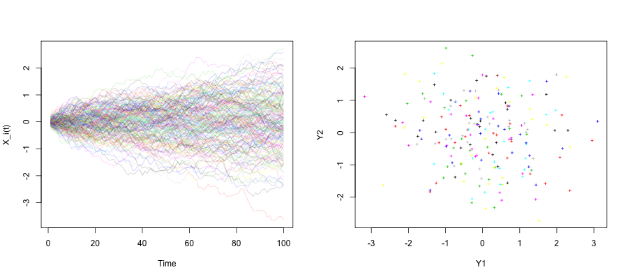
Figure 1: Sample of 200 simulated couples of observations $(X_{i},{\bf Y}_{i})_{i=1,\dots,200}$. The left box contains the covariates $X_{i}$ and in the right one we present their associated vectors ${\bf Y}_{i}$.

We have simulated $n=200,700$ independent realizations $(X_{i},{\bf Y}_{i})$, $i=1,\dots,n.$ To deal with the Brownian random functions $X_{i}(t)$, their sample were discretized by 100 points equispaced in $[0,1]$. In Figure 1, we plot a 200 simulated couples $(X_{i},{\bf Y}_{i})_{i=1,\dots,200}$ as described above. The left box contains the covariates $X_{i}$ and in the right one we present the associated vectors ${\bf Y}_{i}=(Y_{i}^{1},Y_{i}^{2})$.

We aim to assess, for a fixed curve $X=x$, the performance of the asymptotic conditional confidence ellipsoid given by (18) in finite sample. For that we have first to estimate $\mu(x)$. Three parameters should be fixed in this step: the kernel $K$, the bandwidth $h$ and the semimetric $d(\cdot,\cdot)$ which measure the similarity between curves.

Choice of the kernel: there are many possible density kernel functions. Specialists in non-parametric estimation agree that the exact form of the kernel function does not greatly affect the final estimate with regard to the choice of the bandwidth. In this section, the so-called Gaussian kernel will be used, which is defined by $K(u)=(2\pi)^{-1/2}\exp(-u^{2}/2)$, for $u\in\mathbb{R}$.

Choice of the bandwidth $h_{n}$: the bandwidth determines the smoothness of the estimator. The problem of the choice of the bandwidth has been widely studies in non-parametric literature. Recently Rachdi and Vieu (2007) have proposed a data-driven criterion for choosing this smoothing parameter. The proposed criterion can be formulated in terms of a functional version of cross-validation ideas. Antoniadis et al. (2009) treated the same problem in the context of time series prediction. In the following, the bandwidth $h_{n}$ is selected by $L_{1}$ cross-validation method:

$$\widehat{h}_{n,opt}=\arg\min_{h>0}\sum_{i=1}^{n}\left\|{\bf Y}_{i}-\widehat{\mu}_{(-i)}(x_{i})\right\|.$$ (19)

Choice of the semi-metric $d(\cdot,\cdot)$: because of the roughness of our covariate curves we chose a semi-metric computed with the functional principal components analysis with dimension $q=2$.

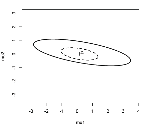
Figure 2: Confidence ellipsoid of $\mu(x)$ when $n=200$ (solid lines) and $n=700$ (dashed lines); the centers of the ellipses at $(\mu_{n}^{1}(x),\mu_{n}^{2}(x))$ are denoted by triangle (n=200) and cross (n=700).

In Figure 2, we plot the $95\%$ confidence ellipses of $\mu(x)$ when $x=0_{\mathcal{F}}$. We can remark from Figure 2 that the lengths of the major and the minor axes of the confidence ellipse decrease when the sample size $n$ increases. Similar results were obtained for other sample sizes $n$ and values of the curve $x.$

4.2 Application to Chemiometrical data prediction

The purpose of this section is to apply our method based on multivariate $L_{1}$-median regression to some chemiometrical real data and to compare our results to those obtained by other definitions of conditional median studied in literature. For that, we used a sample of spectrometric data available on the web site: http://lib.stat.cmu.edu/datasets/tecator. We have a sample of $n=215$ pieces of meat and for each unit $i$, we observe one spectrometric discretized curve $X_{i}(\lambda)$ which corresponds to the absorbance measured at a grid of 100 wavelengths (i.e. $X_{i}(\lambda)=(X_{i}(\lambda_{1}),X_{i}(\lambda_{2}),\dots,X_{i}(\lambda_{100}))$). Figure (3) plots the spectrometric curves. Moreover, for each unit $i$, we have at hand its Moisture content $(Y^{1})$, Fat content $(Y^{2})$ and Protein content $(Y^{3})$ obtained by analytical chemical processing.

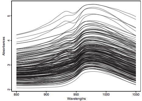
Figure 3: The 215 spectrometric curves.

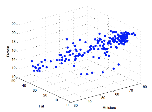
Figure 4: The sample of 215 piece of meat.

Let us denote by ${\bf Y}=(moisture,fat,protein)^{t}:=(Y^{1},Y^{2},Y^{3})^{t}$ the vector of specific chemical contents of meat. Given a new spectrometric curve $X_{new}(\lambda)$, our purpose is to predict simultaneously the corresponding vector of chemical contents $\widehat{\bf Y}$ using the multivariate $L_{1}$-median regression. Obtaining a spectrometric curve is less expensive (in terms of time and cost) than analytical chemistry needed for determining the percentage of chemical contents. So, it is an important economic challenge to predict the hole vector ${\bf Y}$ from the spectrometric curve.

Let us consider 215 observations $(X_{1}(\lambda),{\bf Y}_{1}),\dots,(X_{215}(\lambda),{\bf Y}_{215})$ split into two samples: learning sample (160 observations) and test sample (55 observations). We compare the following three methods, based on multivariate conditional median, to predict the vector of chemical contents ${\bf Y}$ of the test sample. In the following three approaches, we choose the quadratic kernel $K$ defined by:

$$K(u)=\frac{3}{2}(1-u^{2})1\kern-1.99997pt{\rm l}_{[0,1]}.$$

• Non-functional approach (NF)

This method is based on the definition of conditional spatial median studied by Gannoun et al. (2003b) and Cheng and De Gooijer (2007). This approach does not consider the covariate $X$ as a function but a vector of dimension 100 while the response variable ${\bf Y}$ is a vector. For each $i=1,\dots,160$ in the learning sample, the $i^{th}$ vector ${\bf Y}_{i}$ is predicted as follow:

$$\widehat{\bf Y}_{i}=\widehat{\mu}^{NF}(X_{i}),$$

where

$$\widehat{\mu}^{NF}(X_{i})=\mathop{\mathrm{arg\,min}}_{u\in\mathbb{R}^{3}}\sum_{j=1}^{160}w_{n,j}^{NF}(X_{i})\|Y_{j}-u\|,$$

and $w_{n,j}^{NF}(X_{i})=\displaystyle K\left(\frac{X_{i}-X_{j}}{h_{n}}\right)\Big{/}\sum_{j=1}^{n}K\left(\frac{X_{i}-X_{j}}{h_{n}}\right)$ are the so-called Nadaraya-Watson weights. For the choice of the bandwidth $h_{n}$, Cheng and De Gooijer (2007) gave the exact expression of the optimal bandwidth that minimizes the asymptotic mean square error. In this case $h_{n}$ is of the rate $n^{(-1/104+\epsilon)}$, where $\epsilon>0$ is a sufficiently small constant.

• Vector Coordinate Conditional Median (VCCM)

This approach supposes that the covariate $X$ is considered as functional. For each $i=1,\dots,160$ in the learning sample, we predict each component of its vector response ${\bf Y}_{i}$ by the one-dimensional conditional median. Then we obtain the vector of coordinate conditional medians (VCCMs) defined as

$$\widehat{\bf Y}_{i}=(\widehat{\mu}^{1}(X_{i}),\widehat{\mu}^{2}(X_{i}),\widehat{\mu}^{3}(X_{i})),$$

where each component $\widehat{\mu}^{j}(X_{i})=(\widehat{F}^{j})^{-1}(1/2\mid X_{i})$ is the one-dimensional conditional median estimator.

$\widehat{F}^{j}(\cdot\mid X_{i})$ is the conditional distribution function estimator of the component $Y^{j}$ given $X=X_{i}$. Ferraty and Vieu (2006), p. 56, have proposed a Nadaraya-Watson kernel estimator of the conditional distribution, $F^{j}(\cdot\mid X=X_{i})$, when covariate takes values in some infinite dimensional space. This estimator is given by

$$\widehat{F}^{j}(y^{j}\mid X=X_{i})=\sum_{k=1}^{160}1\kern-1.99997pt{\rm l}_{\{Y_{k}^{j}\leq y^{j}\}}K(d(X_{i},X_{k})/h_{n})\Big{/}\sum_{k=1}^{160}K(d(X_{i},X_{k})/h_{n}),\quad y^{j}\in\mathbb{R}.$$

To apply this approach, we used the Ferraty and Vieu’s R/routine funopare.quantile.lcv to estimate $\widehat{\mu}^{j}(X_{i}).$ The optimal bandwidth is chosen by the cross-validation method on the $k$ nearest neighbours (see Ferraty and Vieu (2006), p.102 for more details).

• Conditional Multivariate Median (CMM)

The approach that we propose here supposes the covariate $X$ is a curve and the response $Y$ is a vector. For each $i=1,\dots,160$ in the learning sample we take

$$\widehat{\bf Y}_{i}=\widehat{\mu}(X_{i}),$$

where

$$\widehat{\mu}(X_{i})=\mathop{\mathrm{arg\,min}}_{u\in\mathbb{R}^{3}}\sum_{j=1}^{160}w_{n,j}(X_{i})\|Y_{j}-u\|.$$ (20)

To estimate the conditional multivariate median, $\widehat{\mu}(X_{i})$, we have adapted the algorithm proposed by Vardi and Zhang (2000) to the conditional case and used the function spatial.median from the R package ICSNP. As in the previous approach, the optimal bandwidth is chosen by the cross-validation method on the $k$ nearest neighbours.

A common evaluation procedure:

We have adapted, to the multivariate case, the algorithm proposed by Attouch et al. (2009) and Ferraty and Vieu (2006), p.103) in order to get the optimal smoothing parameter $h_{n}$ for each $X_{i}$ in the test sample.

• We compute the kernel estimator $\widehat{\mu}(X_{j})$ (resp. $\widehat{\mu}^{k}(X_{j})$), for all $j$ by using the training sample.

• For each $X_{i}$ in the test sample, we set $i_{\star}=\mathop{\mathrm{arg\,min}}_{j=1,\dots,160}d(X_{i},X_{j}).$

• For each $i=161,\dots,215$, we take

  $$\widehat{\mu}(X_{i})=\widehat{\mu}(X_{i\star})\quad\mbox{and}\quad\widehat{\mu}^{k}(X_{i})=\widehat{\mu}^{k}(X_{i\star}).$$

The used bandwidth for each curve $X_{i}$ in the test sample is the one obtained for the nearest curve in the learning sample. Because the spectrometric curves presented in Figure (3) are very smooth, we can choose as semi-metric $d(\cdot,\cdot)$ the $L_{2}$ distance between the second derivative of the curves. This choice has been made by Attouch et al. (2009) and Ferraty et al. (2007) for the same spectrometric curves.

Both (CMM) and (NF) methods take into account the covariance structure between variables of of the vector ${\bf Y}$. In fact, the correlation coefficients between $Y_{1}=moisture$, $Y_{2}=fat$ and $Y_{3}=protein$ are given by $\rho_{1,2}=-0.988$, $\rho_{1,3}=0.814$ and $\rho_{2,3}=-0.860$. As we can see moisture, fat and protein contents in meat are strongly correlated then it will be more appropriate to predict these variables simultaneously rather than each one separately.
To compare (CMM), (NF) and (VCCM) methods, we are based on the following criterias:

• The Absolute Error (AE) gives idea about the prediction of each component of ${\bf Y}$

  $$AE_{i}^{j}=|Y_{i}^{j}-\widehat{\mathcal{L}}^{j}(X_{i})|,\quad\quad\forall i=161,\dots,215\quad\mbox{and}\;\;j=1,2,3.$$

• A global criteria ($R$) gives idea about error made to predict the vector ${\bf Y}_{i}$ (for $i=161,\dots,215$)

  $$R(\widehat{\bf Y}_{i})=\|{\bf Y}_{i}-\widehat{\mathcal{L}}(X_{i})\|_{Eucl}$$

where $\widehat{\mathcal{L}}:=(\widehat{\mathcal{L}}^{1},\widehat{\mathcal{L}}^{2},\widehat{\mathcal{L}}^{3})^{t}$ represents the estimator of each component of the vector ${\bf Y}$ obtained by (VCCM), (NF) or (CMM) method.

	CMM				VCCM				NF
	Mean	$Q_{0.25}$	$Q_{0.5}$	$Q_{0.75}$	Mean	$Q_{0.25}$	$Q_{0.5}$	$Q_{0.75}$	Mean	$Q_{0.25}$	$Q_{0.5}$	$Q_{0.75}$
Moist.	1.301	0.479	1.100	2.202	1.776	0.460	1.879	2.383	7.222	1.663	6.374	11.44
Fat	1.565	0.430	1.500	2.401	2.343	0.925	1.716	2.867	9.758	2.328	8.4	15.24
Prot.	1.125	0.300	0.800	1.437	1.313	0.518	1.182	1.806	2.446	0.787	2.329	3.394
$R(\widehat{Y})$	2.638	1.349	2.530	3.623	3.561	1.877	2.909	3.799	12.6	3.523	10.6	19.27

Table 1: Distribution of absolute errors for Moisture, Fat and Protein and global estimation error of the vector ${\bf Y}$.

We can conclude from table 1 that our method is more appropriate to predict meat components than (VCCM). In fact, the (VCCM) approach predicts each component of ${\bf Y}$ separately using conditional univariate median. This method supposes independence of the components of ${\bf Y}$ and doesn’t take into account the correlation structure between variables. The Non-Functional approach gives the most important prediction errors and this is because of the dimension of the covariate (100 in this case). This problem is well-known in nonparametric estimation as curse of dimensionality. Taking into account the functional aspect of the covariate seems to be necessary in such case.

5 Concluding remarks

In this paper, we have introduced a kernel-based estimator for the $L_{1}$-median of a multivariate conditional distribution when covariates take values in an infinite-dimensional space. Prediction using the least square estimates of regression parameters is highly sensitive to outlying points. Therefore, there is no doubt that conditional $L_{1}$-median can be used to make prediction. We have shown that our estimator is well adapted to predict a multivariate response vector. In fact, in contrast to the Vector Coordinate Conditional Median method, the multivariate conditional $L_{1}$-median takes into account the inter-dependance of the coordinates of the response vector. Asymptotic results, i.e., almost sure consistency and asymptotic normality, has been given under some regularity conditions. Many extensions can be given to this work. For instance, the same type of theoretical results could be obtained in a non-independence framework (e.g. mixing dependence). Furthermore, it is well known that quantiles are very useful tools to detect outliers and to modelize the dependence of the covariates in lower and upper tails of the response distribution. In future work, we aim to generalize our study to the multivariate quantiles regression when covariates take values in some infinite dimensional space.

Appendix: Proofs

In order to prove our results we have to introduce some further notations. Let

$$\overline{G}^{x}_{n,2}(u)=\mathbb{E}\left(G_{n,2}^{x}(u)\right):=\frac{1}{\mathbb{E}\Delta_{1}(x)}\mathbb{E}\left[\|Y_{1}-u\|\Delta_{1}(x)\right],$$

and define the bias of $G^{x}_{n}(u)$ as

$$B_{n}^{x}(u)=\overline{G}^{x}_{n,2}(u)-G^{x}(u).$$

Consider now the following quantities

$$R_{n}^{x}(u)=-B_{n}^{x}(u)\left(G^{x}_{n,1}-1\right)$$

and

$$Q_{n}^{x}(u)=\left(G^{x}_{n,2}(u)-\overline{G}_{n,2}^{x}(u)\right)-G^{x}(u)\left(G^{x}_{n,1}-1\right).$$

It is then clear that the following decomposition holds

$$G^{x}_{n}(u)-G^{x}(u)=B_{n}^{x}(u)+\frac{R_{n}^{x}(u)+Q_{n}^{x}(u)}{G^{x}_{n,1}}.$$ (21)

Since $G^{x}_{n,1}$ is independent of $u$, it follows from decomposition (21) that

$$\sup_{u\in\mathbb{R}^{d}}|G^{x}_{n}(u)-G^{x}(u)|\leq\sup_{u\in\mathbb{R}^{d}}|B_{n}^{x}(u)|+\frac{\sup_{u\in\mathbb{R}^{d}}|R_{n}^{x}(u)|+\sup_{u\in\mathbb{R}^{d}}|Q_{n}^{x}(u)|}{G^{x}_{n,1}}.$$ (22)

The proof of Proposition 3.1 is split up into several lemmas, given hereafter, establishing respectively the convergence almost surely (a.s.) of $G^{x}_{n,1}$ to $1$ and that of $B_{n}^{x}(u)$, $R_{n}^{x}(u)$ and $Q_{n}^{x}(u)$ (with rate) to zero.

We start by the following technical lemma whose proof my be found in Ferraty et al. (2007).

Lemma 5.1

Assume that conditions (H1),(H2) hold true. For any real numbers $j\geq 1$ and $k\geq 1,$ as $n\rightarrow\infty$, we have

• $\displaystyle\frac{1}{\phi(h)}\mathbb{E}[\Delta_{1}^{j}(x)]=M_{j}g(x)+o(1)$

• $\displaystyle\frac{1}{\phi^{k}(h)}(\mathbb{E}(\Delta_{1}(x)))^{k}=M_{1}^{k}g^{k}(x)+o(1).$

Lemma below gives the convergence rate of the quantity $G^{x}_{n,1}$.

Lemma 5.2

Under assumptions (H1)-(H2) and condition (10)(i), we have

$$G^{x}_{n,1}-1=O_{a.s}\left(\sqrt{\displaystyle\frac{\log n}{n\phi(h)}}\right).$$

Proof of Lemma 5.2. Let us denote by

$$R^{x}_{n,1}=G^{x}_{n,1}-1:=\frac{1}{n}\sum_{i=1}^{n}L_{n,i}(x),$$

where $L_{n,i}(x)=\Delta_{i}^{\star}(x)-\mathbb{E}(\Delta_{i}^{\star}(x))$ and $\Delta_{i}^{\star}(x)=\frac{\Delta_{i}(x)}{\mathbb{E}(\Delta_{1}(x))}$. To apply the exponential inequality given by Corollary A.8(i) of Ferraty and Vieu (2006) in Appendix A we have first to show that for all $m\geq 2$ there exist a positive constant $C_{m}$ such that $\mathbb{E}|L_{n,1}^{m}(x)|\leq C_{m}a^{2(m-1)}$. We have

$$\mathbb{E}\left(|L_{n,1}(x)|^{m}\right)\leq C\sum_{k=0}^{m}\displaystyle{m\choose k}\mathbb{E}\left[\left(\Delta_{1}^{\star}(x)\right)^{k}\right]\left[\mathbb{E}(\Delta_{1}^{\star}(x))\right]^{m-k}.$$

Then using Lemma 5.1 we get $\mathbb{E}\left(|L_{n,1}(x)|^{m}\right)\leq C_{m}\max_{k=0,1,\dots,m}(\phi(h))^{1-k}\leq C_{m}(\phi(h))^{1-m}.$ Therefore, we have $a^{2}=(\phi(h))^{-1}.$ Now, for all $\epsilon>0$, we have

$$\mathbb{P}(|R^{x}_{n,1}|>\epsilon) \leq 2\exp\left\{-\frac{n\epsilon^{2}}{2\phi(h)(1+\epsilon)}\right\}.$$

The desired result follows from Borel Cantelli Lemma by choosing $\epsilon=\epsilon_{0}\sqrt{\log n/n\phi(h)}$ where $\epsilon_{0}$ is a large enough positive constant.  

The following lemma describes the uniform asymptotic behavior of the conditional bias term $B_{n}^{x}(u)$ as well as that of $R_{n}^{x}(u)$ and $Q_{n}^{x}(u)$ with respect to $u$.

Lemma 5.3

(i) Under conditions (H1)-(H2) (H3)(i), we have

$$\sup_{u\in\mathbb{R}^{d}}|B_{n}^{x}(u)|=O_{a.s.}(h^{\beta}).$$ (23)

(ii) If in addition that (H1)-(H2) hold true and condition (10) is satisfied, we have

$$\sup_{u\in\mathbb{R}^{d}}|R_{n}^{x}(u)|=O_{a.s.}\left(h^{\beta}\sqrt{\frac{\log n}{n\phi(h)}}\right)$$ (24)

Proof of Lemma 5.3. Recall that

$$B_{n}^{x}(u)=\overline{G}^{x}_{n,2}(u)-G^{x}(u).$$

Conditioning by $X$ and using the definition of $G^{x}(u)$ and condition (H3)(i), one has

$$|B_{n}^{x}(u)| = \left|\frac{1}{\mathbb{E}\Delta_{1}(x)}\mathbb{E}\left\{\Delta_{1}(x)\mathbb{E}[\|Y_{1}-u\|\;|\;X]\right\}-G^{x}(u)\right|$$

$$= \left|\frac{1}{\mathbb{E}\Delta_{1}(x)}\mathbb{E}\left\{\Delta_{1}(x)(G^{X}(u)-G^{x}(u))\right\}\right|$$

$$\leq \sup_{x^{\prime}\in B(x,h)}|G^{x^{\prime}}(u)-G^{x}(u)|=O_{a.s.}(h^{\beta}).$$

The later quantity is independent of $u$, this leads to $\sup_{u\in\mathbb{R}^{d}}|B_{n}^{x}(u)|=O_{a.s.}(h^{\beta}).$

Now, to deal with the quantity $R_{n}^{x}(u),$ write it as $R_{n}^{x}(u)=-B_{n}^{x}(u)\left(G^{x}_{n,1}-1\right).$ Therefore

$$\sup_{u\in\mathbb{R}^{d}}|R_{n}^{x}(u)|=\sup_{u\in\mathbb{R}^{d}}|B_{n}^{x}(u)||G^{x}_{n,1}-1|.$$

The statement (24) follows from (23) combined with Lemma 5.2.

 

Lemma 5.4

Under assumptions (H1)-(H2), (H4)(i), conditions (10) and (11) we have

$$\sup_{u\in\mathbb{R}^{d}}|G^{x}_{n,2}(u)-\overline{G}^{x}_{n,2}(u)|=O_{a.s.}\left(\sqrt{\frac{\log n}{n\phi(h)}}\right).$$

Proof of Lemma 5.4. For $u\in\mathbb{R}^{d}$ and $r>0$, let

$$S(u,r)=\{u^{\prime}:u^{\prime}\in\mathbb{R}^{d},||u^{\prime}-u||\leq r\},$$

be the sphere of radius $r$ centered at $u$. Let $[-n^{\gamma},n^{\gamma}]^{d}$, for $1/2<\gamma<2$, be an interval of $\mathbb{R}^{d}$. Divide $[-n^{\gamma},n^{\gamma}]$ into $k_{n}$ subintervals each of length $b_{n}=[2n^{\gamma}/k_{n}]$ (where $[t]$ is the integer part of $t$). Since the set $S(0,n^{\gamma})=\{u^{\prime}:||u^{\prime}||\leq n^{\gamma}\}$ is compact, it can be covered by $k_{n}^{d}$ bounded hypercubes of the form

$$S_{n,j}:=S(u_{j},b_{n})=\{u^{\prime}:||u^{\prime}-u_{j}||\leq b_{n}\},\quad j=1,\ldots,k_{n}^{d}.$$

We have

$$\sup_{||u||\leq n^{\gamma}}|G^{x}_{n,2}(u)-\overline{G}^{x}_{n,2}(u)|$$ (25)

$$\leq \max_{1\leq j\leq k_{n}^{d}}\sup_{u\in S_{n,j}}|G^{x}_{n,2}(u)-G^{x}_{n,2}(u_{j})|+\max_{1\leq j\leq k_{n}^{d}}|G^{x}_{n,2}(u_{j})-\overline{G}^{x}_{n,2}(u_{j})|$$

$$+ \max_{1\leq j\leq k_{n}^{d}}\sup_{u\in S_{n,j}}|\overline{G}^{x}_{n,2}(u)-\overline{G}^{x}_{n,2}(u_{j})|:=I_{n,1}+I_{n,2}+I_{n,3}.$$

Observe now that

$$\sup_{u\in S_{n,j}}|G^{x}_{n,2}(u)-G^{x}_{n,2}(u_{j})| \leq \frac{1}{n\mathbb{E}(\Delta_{1}(x))}\sum_{i=1}^{n}\sup_{u\in S_{n,j}}\Big{|}||Y_{i}-u||-||Y_{i}-u_{j}||\Big{|}\,\Delta_{i}(x)$$

$$\leq \frac{1}{n\mathbb{E}(\Delta_{1}(x))}\sum_{i=1}^{n}\Delta_{i}(x)\sup_{u\in S_{n,j}}||u-u_{j}||=b_{n}G_{n,1}^{x},$$

and

$$\sup_{u\in S_{n,j}}|\overline{G}^{x}_{n,2}(u)-\overline{G}^{x}_{n,2}(u_{j})| \leq \mathbb{E}\left[\sup_{u\in S_{n,j}}|G^{x}_{n,2}(u)-G^{x}_{n,2}(u_{j})|\right]=b_{n}.$$

If we denote by $\alpha_{n}=\sqrt{n\phi(h)/\log n}$ the convergence rate, one gets by Lemma 5.2

$$\alpha_{n}(I_{n,1}+I_{n,3})=\mathcal{O}(\alpha_{n}b_{n}(1+G_{n,1}^{x}))=\mathcal{O}(\alpha_{n}b_{n})=\mathcal{O}(\alpha_{n}n^{\gamma}/k_{n}^{d}).$$

The choice of $k_{n}^{d}=[\alpha_{n}n^{\gamma}\log n]$ implies that

$$\alpha_{n}(I_{n,1}+I_{n,3})=o(1).$$ (26)

In order to evaluate the term $I_{n,2}$, let us denote by

$$\Delta_{i}^{\star}(x)=\frac{\Delta_{i}(x)}{\mathbb{E}\Delta_{1}(x)},$$

and

$$Z_{n,i}(x)=\|Y_{i}-u_{j}\|\Delta_{i}^{\star}(x)-\mathbb{E}\left[\|Y_{1}-u_{j}\|\Delta_{1}^{\star}(x)\right].$$

Then, we have

$$G^{x}_{n,2}(u_{j})-\overline{G}^{x}_{n,2}(u_{j})=\frac{1}{n}\sum_{i=1}^{n}Z_{n,i}(x).$$

For all $m\in\mathbb{N}-\{0\},$ observe that

$$Z_{n,i}^{m}(x)=\sum_{k=0}^{m}\displaystyle{m\choose k}\left(\|Y_{i}-u_{j}\|\Delta_{i}^{\star}(x)\right)^{k}(-1)^{m-k}\left[\mathbb{E}(\|Y_{1}-u_{j}\|\Delta_{1}^{\star}(x))\right]^{m-k}.$$

In order to apply an exponential type inequality, we have to give an upper bound for $\mathbb{E}\left(|Z_{n,1}(x)|^{m}\right)$. It follows from the above inequality that

$$\mathbb{E}\left(|Z_{n,1}(x)|^{m}\right)\leq C\sum_{k=0}^{m}\displaystyle{m\choose k}\mathbb{E}\left[\left(\|Y_{1}-u_{j}\|\Delta_{1}^{\star}(x)\right)^{k}\right]\left[\mathbb{E}(\|Y_{1}-u_{j}\|\Delta_{1}^{\star}(x))\right]^{m-k}.$$

On the other hand, we have for any $k\geq 2$

$$\mathbb{E}\left[\left(\|Y_{1}-u_{j}\|\Delta_{1}^{\star}(x)\right)^{k}\right] = \mathbb{E}\left[(\Delta_{1}^{\star}(x))^{k}\mathbb{E}\left(\|Y_{1}-u_{j}\|^{k}\;|\;X_{1}\right)\right]$$

$$= \mathbb{E}\left[(\Delta_{1}^{\star}(x))^{k}G_{k}^{X_{1}}(u_{j})\right].$$

Using the first part of condition $(H4)(i)$, which implies that $G_{k}^{x}(u_{j})$ is bounded uniformly for all $j$, one may write

$$\mathbb{E}\left[\left(\|Y_{1}-u_{j}\|\Delta_{1}^{\star}(x)\right)^{k}\right] \leq \mathbb{E}\left[(\Delta_{1}^{\star}(x))^{k}|G^{X_{1}}_{k}(u_{j})-G^{x}_{k}(u_{j})|\right]+G^{x}_{k}(u_{j})\mathbb{E}((\Delta_{1}^{\star}(x))^{k})$$

$$\leq \mathbb{E}((\Delta_{1}^{\star}(x))^{k})\left[\max_{j}\sup_{x^{\prime}\in B(x,h)}|G^{x^{\prime}}_{k}(u_{j})-G^{x}_{k}(u_{j})|+\max_{j}G^{x}_{k}(u_{j})\right]$$

$$\leq C_{0}\mathbb{E}\left[(\Delta_{1}^{\star}(x))^{k}\right],$$

where $C_{0}$ is a positive constant. Moreover, we have $\mathbb{E}\left(\|Y_{1}-u_{j}\|\Delta_{1}^{\star}(x)\right)=\mathcal{O}(1)$ uniformly in $j$ since $\mathbb{E}\left[\Delta_{1}^{\star}(x)\right]=1$ and $\sup_{u}\mathbb{E}(||Y_{1}-u||\;|X)<\infty$ in view of condition (2).

Therefore $[\mathbb{E}\left(\|Y_{1}-u_{j}\|\Delta_{1}^{\star}(x)\right)]^{m-k}=\mathcal{O}(1)$.

Next, applying Lemma 5.1, one may write

$$\mathbb{E}\left[(\Delta_{1}^{\star}(x))^{k}\right] = (\phi(h))^{1-k}\left[\frac{M_{k}}{M_{1}^{k}}g^{1-k}(x)+o(1)\right].$$

Thus

$$\mathbb{E}\left(|Z_{n,1}(x)|^{m}\right) \leq C_{m}\max_{k=0,1,\dots,m}(\phi(h))^{1-k}$$

where $C_{m}$ is a real positive constant depending on $m$. Because $\phi(h)$ tends to zero as $n$ goes to infinity, it comes that

$$\mathbb{E}\left(|Z_{n,1}(x)|^{m}\right)=\mathcal{O}\left((\phi(h))^{1-m}\right).$$

Now, applying Corollary $A.8-i$ in Ferraty & Vieu (2006) $k_{n}^{d}$ times with $a^{2}=(\phi(h))^{-1}$ we obtain, by choosing

$$\epsilon=\epsilon_{n}=3\epsilon_{0}\sqrt{v_{n}}\quad\mbox{where}\quad v_{n}=(a^{2}\log n)/n=\log n/(n\phi(h))\longrightarrow 0\quad\mbox{as}\ n\to\infty,$$

that

$$\mathbb{P}\left(|I_{n,2}|\geq\epsilon\right) \leq 2k_{n}^{d}\exp\left(-\epsilon_{0}^{2}\log n\left[\frac{1}{2(1+\epsilon_{0}\sqrt{v_{n}})}\right]\right)\leq 2k_{n}^{d}n^{-\epsilon_{0}^{2}}.$$

One may choose $\epsilon_{0}$ large enough such that

$$\sum_{n}\mathbb{P}\left(|I_{n,2}|\geq\epsilon\right)<\infty.$$

We conclude by Borel-Cantelli lemma and (26) that

$$\alpha_{n}\sup_{||u||\leq n^{\gamma}}|G^{x}_{n,2}(u)-\overline{G}^{x}_{n,2}(u)|=\mathcal{O}_{a.s}(\alpha_{n}\sqrt{v_{n}})=\mathcal{O}_{a.s}(1).$$

Next, we have

$$\sup_{u\in\mathbb{R}^{d}}\alpha_{n}|G^{x}_{n,2}(u)-\overline{G}^{x}_{n,2}(u)| \leq \sup_{||u||\leq n^{\gamma}}\alpha_{n}|G^{x}_{n,2}(u)-\overline{G}^{x}_{n,2}(u)|+\sup_{||u||>n^{\gamma}}\alpha_{n}|G^{x}_{n,2}(u)-\overline{G}^{x}_{n,2}(u)|$$

$$= \sup_{||u||>n^{\gamma}}\alpha_{n}|G^{x}_{n,2}(u)-\overline{G}^{x}_{n,2}(u)|+\mathcal{O}_{a.s.}(1),$$

in view of the above result. Now, we have

$$\alpha_{n}\sup_{u:||u||\geq n^{\gamma}}|G^{x}_{n,2}(u)-\overline{G}^{x}_{n,2}(u)|$$ (27)

$$\leq \alpha_{n}\sup_{u:||u||\geq n^{\gamma}}|G^{x}_{n,2}(u)|+\alpha_{n}\sup_{u:||u||\geq n^{\gamma}}|G^{x}(u)|+\alpha_{n}\sup_{u}|G^{x}(u)-\overline{G}^{x}_{n,2}(u)|.$$

The last term in (27) is zero for large $n$, since conditioning by $X$, one may write

$$\alpha_{n}|\overline{G}_{n,2}^{x}(u)-G^{x}(u)| = \alpha_{n}|B_{n}^{x}(u)|=\mathcal{O}_{a.s.}(h_{n}^{\beta}\alpha_{n})=_{a.s.}(1)$$

in view Lemma 5.3 (i) whenever condition (10)(ii) is satisfied. For the second term in (27), we have

$$\alpha_{n}\sup_{||u||>n^{\gamma}}G^{x}(u)\leq\frac{\alpha_{n}}{n^{\gamma}}\sup_{||u||>n^{\gamma}}||u||G^{x}(u)=o(1),$$

whenever $\gamma>1/2$ and the condition (11) is satisfied.

Moreover, we have for any $\epsilon>0$

$$\mathbb{P}\left\{\alpha_{n}\sup_{u:||u||\geq n^{\gamma}}|G^{x}_{n,2}(u)|\geq\epsilon\right\}$$

$$\leq \mathbb{P}\left\{\alpha_{n}\sup_{u:||u||\geq n^{\gamma}}\frac{1}{n\mathbb{E}(\Delta_{1})}\sum_{i:||Y_{i}-u||>n^{\gamma}/2}||Y_{i}-u||\Delta_{i}(x)||\geq\epsilon/2\right\}$$

$$+ \mathbb{P}\left\{\alpha_{n}\sup_{u:||u||\geq n^{\gamma}}\frac{1}{n\mathbb{E}(\Delta_{1})}\sum_{i:||Y_{i}-u||\leq n^{\gamma}/2}||Y_{i}-u||\Delta_{i}(x)||\geq\epsilon/2\right\}:=J_{n,1}+J_{n,2}.$$

To treat $J_{n,1}$, denote by

$$A_{n}(\omega):=\{\omega:\alpha_{n}\sup_{||u||>n^{\gamma}}\frac{1}{n}\sum_{i=1:||Y_{i}-u||>n^{\gamma}/2}^{n}||Y_{i}-u||\Delta_{i}\geq\epsilon/2\}.$$

The event $A_{n}(\omega)$ is nonempty if and only if there exists at least $i_{0}$ ($1\leq i_{0}\leq n$) such that $||Y_{i_{0}}-u||>n^{\gamma}/2$. Thus $"A_{n}(\omega)\neq\varnothing"\subset\cup_{i=1}^{n}\{\omega:||Y_{i}-u||\geq n^{\gamma}/2\}$. It follows from Markov’s inequality, if $\mathbb{E}(||Y_{1}-u||)<\infty$, that

$$\mathbb{P}\left(A_{n}(\omega)\neq\varnothing\right)=\mathcal{O}(n^{-(\gamma-1)})\quad\mbox{and}\quad\sum_{n}\mathbb{P}\left(A_{n}(\omega)\neq\varnothing\right)<\infty,$$

whenever $\gamma>1$, which implies that $J_{n,1}=o_{a.s.}(1)$ by Borel-Cantelli Lemma.

To deal with $J_{n,2}$, let us denote by

$$B_{n}(\omega):=\{\omega:\alpha_{n}\sup_{u:||u||\geq n^{\gamma}}\frac{1}{n\mathbb{E}(\Delta_{1})}\sum_{i:||Y_{i}-u||\leq n^{\gamma}/2}||Y_{i}-u||\Delta_{i}(x)||\geq\epsilon/2\}.$$

$B_{n}(\omega)$ is nonempty if and only if there exists at least $i_{0}$ ($1\leq i_{0}\leq n$) such that $||Y_{i_{0}}-u||\leq n^{\gamma}/2$. The later inequality implies that $||Y_{i_{0}}-u||-||u||\leq 0$ whenever $||u||\geq n^{\gamma}$. Moreover, we have (by triangle inequality), whenever the above conditions are hold, that

$$||Y_{i_{0}}||\geq\Big{|}||Y_{i_{0}}-u||-||u||\Big{|}=-||Y_{i_{0}}-u||+||u||>n^{\gamma}/2.$$

Therefore,

$$"B_{n}(\omega)\neq\varnothing"\subset\{\exists i_{0}:1\leq i_{0}\leq 1,\ ||Y_{i_{0}}||\geq n^{\gamma}/2\}.$$

We conclude as above that $J_{n,2}=o_{a.s.}(1)$ whenever $E(||Y_{1}||)>\infty$ and $\gamma>1$.

This ends the proof of Lemma 5.4.  

Lemma 5.5

Under assumptions (H1)-(H2), (H4)(i) and condition (10)(i), we have

$$Q_{n}^{x}(u)=\mathcal{O}_{a.s.}\left(\left(\frac{\log n}{n\phi(h)}\right)^{1/2}\right).$$ (28)

Proof of Lemma 5.5. In order to check the statement (28), recall that

$$Q_{n}^{x}(u)=\left(G^{x}_{n,2}(u)-\overline{G}^{x}_{n,2}(u)\right)-G^{x}(u)\left(G^{x}_{n,1}-1\right).$$

The result follows then from Lemmas 5.2 and 5.4.  

Proof of Proposition 3.1. The proof follows from Lemmas 5.2, 5.3, 5.4 and 5.5.

 

Proof of Theorem 3.2.

We have from the definitions of $\mu(x)$ and $\mu_{n}(x)$ and the existence and the uniqueness of these quantities that:

$$G^{x}(\mu(x))=\inf_{u\in\mathbb{R}^{d}}G^{x}(u)\quad\mbox{and}\quad G_{n}^{x}(\mu_{n}(x))=\inf_{u\in\mathbb{R}^{d}}G_{n}^{x}(u).$$

It follows then

$$|G^{x}(\mu(x))-G^{x}(\mu_{n}(x))| \leq |G^{x}(\mu(x))-G_{n}^{x}(\mu_{n})|+|G_{n}^{x}(\mu_{n}(x))-G^{x}(\mu_{n}(x))|$$ (29)

$$= |-(-\inf_{u\in\mathbb{R}^{d}}G^{x}(u)+\inf_{u\in\mathbb{R}^{d}}G_{n}^{x}(u))|+|G_{n}^{x}(\mu_{n}(x))-G^{x}(\mu_{n}(x))|$$

$$= |-\sup_{u\in\mathbb{R}^{d}}G^{x}(u)+\sup_{u\in\mathbb{R}^{d}}G_{n}^{x}(u)|+|G_{n}^{x}(\mu_{n}(x))-G^{x}(\mu_{n}(x))|$$

$$\leq \sup_{u\in\mathbb{R}^{d}}|G^{x}(u)-G_{n}^{x}(u)|+|G_{n}^{x}(\mu_{n}(x))-G^{x}(\mu_{n}(x))|$$

$$\leq 2\sup_{u\in\mathbb{R}^{d}}|G^{x}_{n}(u)-G^{x}(u)|.$$

Moreover, since for any fixed $x\in{\cal F}$, the function $G^{x}(\cdot)$ is uniformly continuous and because $\mu(x)$ is the unique minimizer of the function $G^{x}(\cdot)$, we have then, for any $\epsilon>0,$

$$\inf_{u:\|\mu(x)-u\|\geq\epsilon}G^{x}(u)>G^{x}(\mu(x)),$$ (30)

which means that there exists for every $\epsilon>0$, a number $\eta(\epsilon)>0$ such that $G^{x}(u)>G^{x}(\mu(x))+\eta(\epsilon)$ for every $u$ such that $\|\mu(x)-u\|\geq\epsilon.$ This implies that the event $\{\|\mu(x)-\mu_{n}(x)\|>\epsilon\}$ is included in the event $\{G^{x}(\mu_{n}(x))>G^{x}(\mu(x))+\eta(\epsilon)\}.$

Using inequality (29) we get

$$\sum_{n\geq 1}\mathbb{P}\left(\|\mu_{n}(x)-\mu(x)\|>\epsilon\right) \leq \sum_{n\geq 1}\mathbb{P}\left(G^{x}(\mu_{n}(x))>G^{x}(\mu(x))+\eta(\epsilon)\right)$$

$$\leq \sum_{n\geq 1}\mathbb{P}\left(\sup_{u\in\mathbb{R}^{d}}|G_{n}^{x}(u)-G^{x}(u)|>\eta(\epsilon)/2\right)<\infty,$$

similarly to the proof of the Proposition 3.1. The statement (12) follows then from an application of Borel-Cantelli Lemma.  

Proof of Proposition 3.2

To prove Proposition 3.2, it suffices to see that

$$\|\widetilde{H}_{n}^{x}(\xi_{n}(j))-H^{x}(\mu)\|\leq\|\widetilde{H}_{n}^{x}(\xi_{n}(j))-\widetilde{H}_{n}^{x}(\mu)\|+\|\widetilde{H}_{n}^{x}(\mu)-H^{x}(\mu)\|.$$ (31)

Concerning the first term, observe that

$$\|\widetilde{H}_{n}^{x}(\xi_{n}(i))-\widetilde{H}_{n}^{x}(\mu)\| \leq \frac{1}{n\;\mathbb{E}(\Delta_{1}(x))}\sum_{i=1}^{n}\|\mathcal{M}(Y_{i},\xi_{n}(j))-\mathcal{M}(Y_{i},\mu)\|\;\Delta_{i}(x)$$ (32)

$$:= \mathcal{A}_{n}+\mathcal{B}_{n},$$

where

$$\mathcal{A}_{n}:=\frac{\sqrt{d}}{n\mathbb{E}(\Delta_{1}(x))}\sum_{i=1}^{n}\frac{\Big{|}\|Y_{i}-\mu\|-\|Y_{i}-\xi_{n}(j)\|\Big{|}\Delta_{i}(x)}{\|Y_{i}-\mu\|\;\|Y_{i}-\xi_{n}(j)\|}$$

and

$$\mathcal{B}_{n}:=\frac{1}{n\mathbb{E}(\Delta_{1}(x))}\sum_{i=1}^{n}\Delta_{i}(x)\frac{\Big{|}\Big{|}\|Y_{i}-\xi_{n}(j)\|\;\mathcal{U}(Y_{i}-\mu)\;\mathcal{U}^{T}(Y_{i}-\mu)-\|Y_{i}-\mu\|\;\mathcal{U}(Y_{i}-\xi_{n}(j))\;\mathcal{U}^{T}(Y_{i}-\xi_{n}(j))\Big{|}\Big{|}}{\|Y_{i}-\mu\|\;\|Y_{i}-\xi_{n}(j)\|}.$$

Using Theorem 3.2 and the triangular inequality we can easily see that $\mathcal{A}_{n}=o_{a.s.}(1)\times\frac{1}{n\mathbb{E}(\Delta_{1}(x))}\sum_{i=1}^{n}\frac{\Delta_{i}(x)}{\|Y_{i}-\mu\|^{2}}$.

Combining Markov and Cauchy-Schwarz inequalities and making use of the assumption H3-(iii), we can easily prove that $\frac{1}{n\mathbb{E}(\Delta_{1}(x))}\sum_{i=1}^{n}\frac{\Delta_{i}(x)}{\|Y_{i}-\mu\|^{2}}=\mathcal{O}_{\mathbb{P}}(1)$. Then we conclude that $\mathcal{A}_{n}=o_{\mathbb{P}}(1).$

For the second term $\mathcal{B}_{n}$ of the inequality (32), we have by triangular inequality and the fact that $\|U(Y_{i}-\theta)\|=1$, that

$$\Big{|}\Big{|}\|Y_{i}-\xi_{n}(j)\|\;\mathcal{U}(Y_{i}-\mu)\;\mathcal{U}^{T}(Y_{i}-\mu)-\|Y_{i}-\mu\|\;\mathcal{U}(Y_{i}-\xi_{n}(j))\;\mathcal{U}^{T}(Y_{i}-\xi_{n}(j))\Big{|}\Big{|} \leq$$

$$\Big{|}\|Y_{i}-\xi_{n}(j)\|-\|Y_{i}-\mu\|\Big{|}+\|Y_{i}-\mu\|\;\Big{|}\Big{|}\mathcal{U}(Y_{i}-\mu)\;\mathcal{U}^{T}(Y_{i}-\mu)-\mathcal{U}(Y_{i}-\xi_{n}(j))\;\mathcal{U}^{T}(Y_{i}-\xi_{n}(j))\Big{|}\Big{|} \leq$$

$$\|\mu-\xi_{n}(j)\|+\|Y_{i}-\mu\|\times\Big{|}\Big{|}\,\mathcal{U}(Y_{i}-\mu)\;\mathcal{U}^{T}(Y_{i}-\mu)-\mathcal{U}(Y_{i}-\xi_{n}(j))\;\mathcal{U}^{T}(Y_{i}-\xi_{n}(j))\Big{|}\Big{|}.$$

Since

$$\mathcal{U}(Y_{i}-\mu)\,\mathcal{U}^{T}(Y_{i}-\mu)-\mathcal{U}(Y_{i}-\xi_{n}(j))\,\mathcal{U}^{T}(Y_{i}-\xi_{n}(j)) = \left[\,\mathcal{U}(Y_{i}-\mu)-\mathcal{U}(Y_{i}-\xi_{n}(j))\,\right]\,\mathcal{U}^{T}(Y_{i}-\mu)$$

$$+\;\mathcal{U}(Y_{i}-\xi_{n}(j))\left[\,\mathcal{U}^{T}(Y_{i}-\mu)-\mathcal{U}^{T}(Y_{i}-\xi_{n}(j))\,\right],$$

and $\displaystyle\|\mathcal{U}(Y_{i}-\mu)-\mathcal{U}(Y_{i}-\xi_{n}(j))\|\leq 2\frac{\|\mu-\xi_{n}(j)\|}{\|Y_{i}-\xi_{n}(j)\|}$, we can conclude, by using Theorem 3.2, that

$$\mathcal{B}_{n}=o_{a.s.}(1)\times\frac{1}{n\mathbb{E}(\Delta_{1}(x))}\sum_{i=1}^{n}\frac{\Delta_{i}(x)}{\|Y_{i}-\mu\|^{2}}$$

Finally, using the same arguments as above (concerning the proof of the term $\mathcal{A}_{n}$), we get $\mathcal{B}_{n}=o_{\mathbb{P}}(1)$ and this is allows us to conclude that $\|\widetilde{H}_{n}^{x}(\xi_{n}(i))-\widetilde{H}_{n}^{x}(\mu)\|=o_{\mathbb{P}}(1)$. Now we are interesting to the second term of the right side term of (31). Write

$$\widetilde{H}_{n}^{x}(\mu)-H^{x}(\mu)=\underbrace{\widetilde{H}_{n}^{x}(\mu)-\mathbb{E}[\widetilde{H}_{n}^{x}(\mu)]}_{K_{n,1}}+\underbrace{\mathbb{E}[\widetilde{H}_{n}^{x}(\mu)]-H^{x}(\mu)}_{K_{n,2}}.$$

We have to show that each term $K_{n,i}$ $(i=1,2)$ is asymptotically negligible. We have

$$\|K_{n,1}\|^{2}=tr(K_{n,1}^{T}K_{n,1})=\sum_{k=1}^{d}\sum_{j=1}^{d}\mathcal{Z}_{k,j}^{2}$$

where $(\mathcal{Z}_{k,j})_{1\leq k,j\leq d}$ is the general term of the matrix $K_{n,1}^{T}K_{n,1}$ which may be can be written as

$$\mathcal{Z}_{k,j} = \frac{1}{n\mathbb{E}(\Delta_{1}(x))}\sum_{i=1}^{n}\left[\mathcal{M}_{k,j}(Y_{i},\mu)\Delta_{i}(x)-\mathbb{E}\left(\mathcal{M}_{k,j}(Y_{i},\mu)\Delta_{i}(x)\right)\right].$$

Using the assumption (H3)-(iv), Lemma 5.1 and corollary A.8 of Ferraty and Vieu (2006), we can easily prove that for all $1\leq k,j\leq d$, $Z_{k,j}=o_{\mathbb{P}}(1)$.

To handle $K_{n,2}$, observe that

$$\|K_{n,2}\| = \left\|\mathbb{E}\left[\frac{\sum_{i=1}^{n}\mathcal{M}(Y_{i},\mu)\;\Delta_{i}(x)}{n\;\mathbb{E}(\Delta_{1}(x))}\right]-H^{x}(\mu)\right\|$$

$$\leq \frac{1}{\mathbb{E}(\Delta_{1}(x))}\mathbb{E}\left(\|H^{X_{1}}(\mu)-H^{x}(\mu)\|\Delta_{1}(x)\right)$$

$$\leq \sup_{x^{\prime}\in B(x,h)}\|H^{x^{\prime}}(\mu)-H^{x}(\mu)\|=o_{a.s.}(1)$$

in view of condition $(H3)(ii)$.  

Lemma 5.6

Under hypothesis (H1)-(H2) and (H4)(ii), and if for any $\delta>0$, $(n\phi(h))^{-\delta/2}\rightarrow 0$, we have

$$\sqrt{n\phi(h)}\left(\nabla_{u}\widetilde{G}_{n}^{x}(\mu)-\mathbb{E}\left[\nabla_{u}\widetilde{G}_{n}^{x}(\mu)\right]\right)\stackrel{{\scriptstyle\mathcal{D}}}{{\longrightarrow}}\mathcal{N}_{d}(0,\ \tilde{\Sigma}^{x}(\mu)).$$

where $\tilde{\Sigma}^{x}(\mu)$ is the limiting covariance matrix of $\nabla_{u}\widetilde{G}_{n}^{x}(\mu)-\mathbb{E}\left[\nabla_{u}\widetilde{G}_{n}^{x}(\mu)\right].$

Proof of Lemma 5.6. Let’s denote by

$$A_{i}=\frac{\sqrt{\phi(h)}}{\mathbb{E}(\Delta_{1}(x))}\times\mathcal{U}(Y_{i}-\mu)\;\Delta_{i}(x)$$

Then

$$\sqrt{n\phi(h)}\left(\nabla_{u}\widetilde{G}_{n}^{x}(\mu)-\mathbb{E}\left[\nabla_{u}\widetilde{G}_{n}^{x}(\mu)\right]\right)=\frac{1}{\sqrt{n}}\sum_{i=1}^{n}(A_{i}-\mathbb{E}(A_{i})):=\frac{1}{\sqrt{n}}\sum_{i=1}^{n}\widetilde{A}_{i}.$$

From the Cramer-Wold device, Lemma 5.6 can be proved by finding the limit distribution of the real variables sequence $\frac{1}{\sqrt{n}}\sum_{i=1}^{n}\ell^{t}\;\widetilde{A}_{i}$, for all $\ell\in\mathbb{R}^{d}$ satisfying $\|l\|\neq 0$.

Because the random variables $\ell^{t}\widetilde{A}_{1},\dots,\ell^{t}\widetilde{A}_{n}$ are i.i.d. with zero mean and asymptotic variance

$$\sigma^{2}(x) = \lim_{n\rightarrow\infty}Var\left({\frac{1}{\sqrt{n}}\sum_{i=1}^{n}\ell^{t}\;\widetilde{A}_{i}}\right).$$

The result may be obtained by applying the Liapounov Central Theorem Limit. For this propose, we have to prove the following Lindeberg condition:

$$\forall\delta>0\quad\left[n\;\ell^{t}\widetilde{\Sigma}^{x}(\mu)\ell\right]^{-(2+\delta)/2}\sum_{i=1}^{n}\mathbb{E}|\ell^{t}\widetilde{A}_{i}|^{2+\delta}\longrightarrow 0\quad\mbox{as}\quad n\longrightarrow\infty.$$

It is easy to see that:

$$\left[n\;\ell^{t}\widetilde{\Sigma}^{x}(\mu)\ell\right]^{-(2+\delta)/2}\sum_{i=1}^{n}\mathbb{E}|\ell^{t}\widetilde{A}_{i}|^{2+\delta} = n^{-\delta/2}\left(\ell^{t}\Sigma^{x}(\mu)\ell\right)^{-(2+\delta)/2}\mathbb{E}|\ell^{t}\widetilde{A}_{1}|^{2+\delta}.$$

Moreover, using $C_{r}$ and Jensen inequalities, we obtain

$$\mathbb{E}|\ell^{t}\widetilde{A}_{1}|^{2+\delta} \leq c\frac{(\phi(h))^{(2+\delta)/2}}{(\mathbb{E}\Delta_{1}(x))^{2+\delta}}\mathbb{E}\left|\ell^{t}\left(\mathcal{U}(Y_{1}-\mu)\right)^{2+\delta}\times\Delta_{1}^{2+\delta}(x)\right|$$

$$\leq c\frac{(\phi(h))^{(2+\delta)/2}}{(\mathbb{E}\Delta_{1}(x))^{2+\delta}}\mathbb{E}\left\{\Delta_{1}^{2+\delta}(x)\;\underbrace{\mathbb{E}\left[\left|\ell^{t}\mathcal{U}(Y_{1}-\mu)\right|^{2+\delta}\;|\;X\right]}_{=W_{2+\delta}^{X}(\mu)}\right\}$$

$$\leq c\frac{(\phi(h))^{(2+\delta)/2}}{(\mathbb{E}\Delta_{1}(x))^{2+\delta}}\left[\mathbb{E}(\Delta_{1}(x))^{2+\delta}\sup_{x^{\prime}\in B(x,h)}|W_{2+\delta}^{x^{\prime}}(\mu)-W_{2+\delta}^{x}(\mu)|+W_{2+\delta}^{x}(\mu)\mathbb{E}(\Delta_{1}(x))^{2+\delta}\right].$$

It follows then, by hypothesis (H4)(ii) and Lemma 5.1, that

$$\mathbb{E}|\ell^{t}\widetilde{A}_{1}|^{2+\delta} \leq c\frac{(\phi(h))^{(2+\delta)/2}}{(\mathbb{E}\Delta_{1}(x))^{2+\delta}}W_{2+\delta}^{x}(\mu)\mathbb{E}(\Delta_{1}(x))^{2+\delta}$$

$$\leq c^{\prime}\frac{\left(\phi(h)\right)^{(2+\delta)/2}}{\left(\phi(h)\right)^{(2+\delta)}[M_{1}^{2+\delta}(g(x))^{2+\delta}+o(1)]}\left[\phi(h)(M_{(2+\delta)/2}g(x)+o(1))\right]$$

$$= \mathcal{O}\left((\phi(h)^{-\delta/2})\right).$$

Finally, since $(\ell^{t}\widetilde{\Sigma}^{x}(\mu)\ell)^{-(2+\delta)/2}$ is finite, it comes that

$$\left[n\;\ell^{t}\widetilde{\Sigma}^{x}(\mu)\ell\right]^{-(2+\delta)/2}\sum_{i=1}^{n}\mathbb{E}|\ell^{t}\widetilde{A}_{i}|^{2+\delta}=\mathcal{O}\left((n\phi(h)^{-\delta/2})\right)=o(1),$$

because $n\phi(h)\rightarrow\infty$ as $n\rightarrow\infty$. This implies the Lindeberg condition, which completes the proof of the Lemma.  

The following Lemma gives the analytic expression of the matrix $\Sigma^{x}(\mu)$.

Lemma 5.7

Under conditions (H1)-(H2) and (H4)(ii), we have

$$\sigma^{2}(x)=\lim_{n\rightarrow\infty}Var\left({\frac{1}{\sqrt{n}}\sum_{i=1}^{n}\ell^{t}\;\widetilde{A}_{i}}\right)=\frac{M_{2}}{M_{1}^{2}g(x)}\;\ell^{t}\Sigma^{x}(\mu)\ell.$$

Proof of Lemma 5.7. Since the random variables $(\ell^{t}\widetilde{A}_{i})_{i=1,\dots,n}$ are i.i.d. with mean zero, it follows that

$$\sigma^{2}(x)=\lim_{n\rightarrow\infty}Var\left({\frac{1}{\sqrt{n}}\sum_{i=1}^{n}\ell^{t}\;\widetilde{A}_{i}}\right)=\lim_{n\rightarrow\infty}Var(\ell^{t}\widetilde{A}_{1})=\lim_{n\rightarrow\infty}\mathbb{E}\left((\ell^{t}A_{1})^{2}\right).$$

On the other hand, making use of the properties of conditional expectation one may write

$$\mathbb{E}\left[\left(\ell^{t}A_{1}\right)^{2}\right] = \frac{\phi(h)}{(\mathbb{E}\Delta_{1})^{2}}\;\mathbb{E}\left[\Delta_{1}\ell^{t}\mathcal{U}(Y_{1}-\mu)\right]^{2}=\frac{\phi(h)}{(\mathbb{E}\Delta_{1})^{2}}\;\mathbb{E}\left[\Delta^{2}_{1}W_{2}^{X_{1}}(\mu)\right]$$

Making use of the condition (H4)(ii) and the fact that the functions $W_{2}^{x}(\cdot)$ is bounded, we obtain

$$\mathbb{E}\left\{\Delta^{2}_{1}W_{2}^{X_{1}}(\mu)\right\} = \mathbb{E}\left(\Delta^{2}_{1}\right)\left[W_{2}^{x}(\mu)+\mathcal{O}\left(\sup_{u\in\mathbb{R}^{d}}|W^{u}_{2}(\mu)-W^{x}_{2}(\mu)|\right)\right]$$

$$= W_{2}^{x}(\mu)\mathbb{E}\left(\Delta^{2}_{1}\right)+o\left(\mathbb{E}\left(\Delta^{2}_{1}\right)\right).$$

Using Lemma 5.1, one may see that

$$\frac{\phi(h)}{(\mathbb{E}\Delta_{1})^{2}}\mathbb{E}(\Delta_{1}^{2})=\frac{M_{2}}{M_{1}^{2}g(x)}+o(1).$$

Therefore,

$$\sigma^{2}(x)=\frac{M_{2}}{M_{1}^{2}g(x)}W_{2}^{x}(\mu)+o(1).$$

 

Proof of Proposition 3.3. For each $x\in\mathcal{F}$, since $(X_{i},Y_{i})_{i=1,\dots,n}$ are i.i.d., we have

$$\widetilde{\mathcal{B}}_{n}(x)=\mathbb{E}\left[\nabla_{u}\widetilde{G}_{n}^{x}(\mu)\right]=\frac{\mathbb{E}\left[\mathcal{U}(Y_{1}-\mu)\Delta_{1}(x)\right]}{\mathbb{E}(\Delta_{1}(x))}$$

By conditioning with respect to real variable $d(x,X_{1})$ and using condition (H5), we have

$$\widetilde{\mathcal{B}}_{n}(x)=\frac{\mathbb{E}\left[K\left(\frac{d(x,X_{1})}{h}\right)\psi(d(x,X_{1}))\right]}{\mathbb{E}\left(K\left(\frac{d(x,X_{1})}{h}\right)\right)}.$$

Integration with respect to the distribution of the real variable $d(x,X_{1})$ shows that

$$A_{1}:=\mathbb{E}\left[K\left(\frac{d(x,X_{1})}{h}\right)\psi(d(x,X_{1}))\right]=\int_{0}^{1}K(t)\psi(th)dF(th),$$

where $F$ is the cumulative distribution function of the real random variable $d(x,X)$. On the other hand, Taylor series expansion of the function $\psi$ up to the order one in the neighborhood of $t=0$ gives $\psi(th)=th\nabla\psi(0)+o_{d}(h).$ Let us denote by $o_{d}(1)$ (resp. $\mathcal{O}_{d}(1)$) a d-dimensional vector where each component equal to $o(1)$ (resp. $\mathcal{O}(1)$).

Therefore, we have

$$A_{1} = h\nabla\psi(0)\int_{0}^{1}tK(t)dF_{x}(th)+o_{d}(h)\int_{0}^{1}K(t)dF(th)$$

$$= h\nabla\psi(0)\left[K(1)F(h)-\int_{0}^{1}(sK(s))^{\prime}F(sh)ds\right]+o_{d}(h)\left[K(1)F(h)-\int_{0}^{1}K^{\prime}(s)F(sh)ds\right].$$

Using hypothesis $(H2)(i)-(ii)$ we get

$$A_{1} = h\nabla\psi(0)K(1)\left(\phi(h)g(x)+o(\phi(h))\right)-h\nabla\psi(0)\int_{0}^{1}(sK(s))^{\prime}\left(\phi(sh)g(x)+o(\phi(hs))\right)ds$$

$$+o(h)K(1)\left(\phi(h)g(x)+o(\phi(h))\right)-o_{d}(h)\int_{0}^{1}K^{\prime}(s)\left(\phi(sh)g(x)+o(\phi(sh))\right)ds$$

$$= h\phi(h)g(x)\nabla\psi(0)\left[K(1)-\int_{0}^{1}(sK(s))^{\prime}\left(\tau_{0}(s)+o(1)\right)ds\right]+h\phi(h)K(1)o_{d}(1)$$

$$-o_{d}(h\phi(h))\int_{0}^{1}K^{\prime}(s)(\tau_{0}(s)g(x)+o(1))ds$$

$$= h\phi(h)g(x)\nabla\psi(0)\left[K(1)-\int_{0}^{1}(sK(s))^{\prime}\tau_{0}(s)ds\right]+O_{d}^{a.s.}(h\phi(h))$$

Thus, making use of the Lemma 5.1, we obtain

$$\widetilde{\mathcal{B}}_{n}(x)=\frac{h\nabla\psi(0)}{M_{1}}\left[K(1)-\int_{0}^{1}(sK(s))^{\prime}\tau_{0}(s)ds+o_{a.s.}(1)\right]$$

 

Proof of Theorem 3.3

Part (i) follows from Proposition 3.2, decomposition (17), Proposition 5.6 and Lemma 5.7.

Part (ii) follows from Proposition 3.3 combined with the condition $\sqrt{n\phi(h)}h\longrightarrow 0$ as $n\rightarrow\infty$.

 
Proof of Corollary 3.5. Let us denote by

$$T^{x}(\mu)=\left[\Sigma^{x}(\mu)\right]^{-1/2}H^{x}(\mu),\quad T_{n}^{x}(\mu_{n})=\left[\Sigma_{n}^{x}(\mu_{n})\right]^{-1/2}H_{n}^{x}(\mu_{n})$$

and

$$V_{n}^{x}(\mu_{n})=\frac{M_{1,n}}{\sqrt{M_{2,n}}}\sqrt{nF_{x,n}(h)}\;\;T_{n}^{x}(\mu_{n})\left(\mu_{n}-\mu\right).$$

Write

$$V_{n}^{x}(\mu_{n}) = \frac{M_{1,n}\sqrt{M_{2}}}{M_{1}\sqrt{M_{2,n}}}\;\sqrt{nF_{x,n}(h)\left(n\phi(h)g(x)\right)^{-1}}\;T_{n}^{x}(\mu_{n})\;\left[T^{x}(\mu)\right]^{-1}\times\frac{M_{1}}{\sqrt{M_{2}}}\sqrt{n\phi(h)g(x)}\;T^{x}(\mu)\left(\mu_{n}-\mu\right)$$ (33)

$$:= V_{n,1}^{x}\times V_{n,2}^{x}.$$

Making use of Theorem 3.3 part (ii), the term $V_{n,2}^{x}$ converges in distribution to ${\cal N}(0,I_{d})$.

Now to get the result of the corollary it suffices to show that the first term $V_{n,1}^{x}$ converges to 1 in probability. Following the same arguments as in Laïb and Louani (2010) combined with (H1),(H2), one gets

$\displaystyle\frac{M_{1,n}\sqrt{M_{2}}}{M_{1}\sqrt{M_{2,n}}}\;\sqrt{nF_{x,n}(h)\left(n\phi(h)g(x)\right)^{-1}}\stackrel{{\scriptstyle\mathbb{P}}}{{\longrightarrow}}1$, $M_{1,n}\stackrel{{\scriptstyle\mathbb{P}}}{{\longrightarrow}}M_{1}$ and $M_{2,n}\stackrel{{\scriptstyle\mathbb{P}}}{{\longrightarrow}}M_{2}$, as $n\rightarrow\infty$.

Now, we have to establish the consistency of $T_{n}^{x}(\mu_{n})$. To do that, we will study separately the consistency of each term of $T_{n}^{x}(\mu_{n})$. Let us start by $H_{n}^{x}(\mu_{n})$. For this, write

$$H_{n}^{x}(\mu_{n})-H^{x}(\mu) = \frac{\widetilde{H}_{n}^{x}(\mu_{n})}{G_{n,1}^{x}}-H^{x}(\mu)$$

$$= \frac{\widetilde{H}_{n}^{x}(\mu_{n})-H(\mu)}{G_{n,1}^{x}}+\frac{H^{x}(\mu)(1-G_{n,1}^{x})}{G_{n,1}^{x}}.$$

According to Theorem 3.2, Proposition 3.2, Lemma 5.2 and the fact that the matrix $H^{x}(\mu)$ is bounded, we can conclude that $H_{n}^{x}(\mu_{n})$ converges, in probability, to $H^{x}(\mu)$.

The second term $\Sigma_{n}^{x}(\mu_{n})$, can be treated similarly. Finally, this leads to the convergence in probability of $T_{n}^{x}(\mu_{n})$ to $T^{x}(\mu)$.

References

- Abdous and Theodorescu (1992) Abdous, B. and Theodorescu, R. (1992). Note on the spatial quantile of a random vector. Statist. Probab. Lett., 13(4), 333–336.
- Antoniadis et al. (2009) Antoniadis, A., Paparoditis, E., and Sapatinas, T. (2009). Bandwidth selection for functional time series prediction. Statist. Probab. Lett., 79(6), 733–740.
- Ash and Gardner (1975) Ash, R. B. and Gardner, M. F. (1975). Topics in stochastic processes. Academic Press [Harcourt Brace Jovanovich Publishers], New York. Probability and Mathematical Statistics, Vol. 27.
- Attouch et al. (2009) Attouch, M., Laksaci, A., and Ould-Saïd, E. (2009). Asymptotic distribution of robust estimator for functional nonparametric models. Comm. Statist. Theory Methods, 38(8-10), 1317–1335.
- Besse et al. (2000) Besse, P., C. H., , and Stephenson, D. (2000). Autoregressive forecasting of some functional climatic variations. J. Nonparametr. Statist., 27, 673–687.
- Bosq (1996) Bosq, D. (1996). Nonparametric statistics for stochastic processes, volume 110 of Lecture Notes in Statistics. Springer-Verlag, New York. Estimation and prediction.
- Bosq (2000) Bosq, D. (2000). Linear processes in function spaces, volume 149 of Lecture Notes in Statistics. Springer-Verlag, New York. Theory and applications.
- Cadre (2001) Cadre, B. (2001). Convergent estimators for the -median of a Banach valued random variable. Statistics, 35(4), 509–521.
- Cardot et al. (2005) Cardot, H., Crambes, C., and Sarda, P. (2005). Quantile regression when the covariates are functions. J. Nonparametr. Stat., 17(7), 841–856.
- Chaudhuri (1992) Chaudhuri, P. (1992). Multivariate location estimation using extension of -estimates through -statistics type approach. Ann. Statist., 20(2), 897–916.
- Chaudhuri (1996) Chaudhuri, P. (1996). On a geometric notion of quantiles for multivariate data. J. Amer. Statist. Assoc., 91(434), 862–872.
- Chebana and Ouarda (2011) Chebana, F. and Ouarda, T. B. M. J. (2011). Multivariate quantiles in hydrological frequency analysis. Environmetrics, 22(1), 63–78.
- Cheng and De Gooijer (2007) Cheng, Y. and De Gooijer, J. G. (2007). On the th geometric conditional quantile. J. Statist. Plann. Inference, 137(6), 1914–1930.
- Dabo-Niang and Laksaci (2012) Dabo-Niang, S. and Laksaci, A. (2012). Nonparametric quantile regression estimation for functional dependent data. Comm. Statist. Theory Methods, 41(7), 1254–1268.
- De Gooijer et al. (2006) De Gooijer, J. G., Gannoun, A., and Zerom, D. (2006). A multivariate quantile predictor. Comm. Statist. Theory Methods, 35(1-3), 133–147.
- Ezzahrioui and Ould-Saïd (2008) Ezzahrioui, M. and Ould-Saïd, E. (2008). Asymptotic results of a nonparametric conditional quantile estimator for functional time series. Comm. Statist. Theory Methods, 37(16-17), 2735–2759.
- Ferraty and Vieu (2006) Ferraty, F. and Vieu, P. (2006). Nonparametric functional data analysis. Springer Series in Statistics. Springer, New York. Theory and practice.
- Ferraty et al. (2005) Ferraty, F., Rabhi, A., and Vieu, P. (2005). Conditional quantiles for dependent functional data with application to the climatic El Niño phenomenon. Sankhyā, 67(2), 378–398.
- Ferraty et al. (2007) Ferraty, F., Mas, A., and Vieu, P. (2007). Nonparametric regression on functional data: inference and practical aspects. Aust. N. Z. J. Stat., 49(3), 267–286.
- Gannoun et al. (2003a) Gannoun, A., Saracco, J., and Yu, K. (2003a). Nonparametric prediction by conditional median and quantiles. J. Statist. Plann. Inference, 117(2), 207–223.
- Gannoun et al. (2003b) Gannoun, A., Saracco, J., Yuan, A., and Bonney, G. E. (2003b). On adaptive transformation-retransformation estimate of conditional spatial median. Comm. Statist. Theory Methods, 32(10), 1981–2011.
- Gasser et al. (1998) Gasser, T., Hall, P., and Presnell, B. (1998). Nonparametric estimation of the mode of a distribution of random curves. J. R. Stat. Soc. Ser. B Stat. Methodol., 60(4), 681–691.
- Haldane (1948) Haldane, J. (1948). Note on the median of a multivariate distribution. Biometrika, 35, 414–415.
- Hastie and Mallows (1993) Hastie, T. and Mallows, C. (1993). A discussion of “a statistical view of some chemometrics regression tools” by i.e. frank & j.h. friedman. Technometrics, 35, 140–143.
- Kemperman (1987) Kemperman, J. H. B. (1987). The median of a finite measure on a Banach space. In Statistical data analysis based on the -norm and related methods (Neuchâtel, 1987), pages 217–230. North-Holland, Amsterdam.
- Kirkpatrick and Heckman (1989) Kirkpatrick, M. and Heckman, N. (1989). A quantitative genetic model for growth, shape, reaction norms, and other infinite-dimensional characters. J. Math. Biol., 27(4), 429–450.
- Kneip and Utikal (2001) Kneip, A. and Utikal, K. J. (2001). Inference for density families using functional principal component analysis. J. Amer. Statist. Assoc., 96(454), 519–542. With comments and a rejoinder by the authors.
- Koltchinskii (1997) Koltchinskii, V. I. (1997). -estimation, convexity and quantiles. Ann. Statist., 25(2), 435–477.
- Laïb and Louani (2010) Laïb, N. and Louani, D. (2010). Nonparametric kernel regression estimation for functional stationary ergodic data: asymptotic properties. J. Multivariate Anal., 101(10), 2266–2281.
- Laïb and Louani (2011) Laïb, N. and Louani, D. (2011). Rates of strong consistencies of the regression function estimator for functional stationary ergodic data. J. Statist. Plann. Inference, 141(1), 359–372.
- Laksaci et al. (2009) Laksaci, A., Lemdani, M., and Ould-Saïd, E. (2009). A generalized -approach for a kernel estimator of conditional quantile with functional regressors: consistency and asymptotic normality. Statist. Probab. Lett., 79(8), 1065–1073.
- Lipster and Shiryayev (1972) Lipster, R. and Shiryayev, A. (1972). On the absolute continuity of measures corresponding to processes of diffusion type relative to awiener measure. Izv. Akad. Nauk. Ser. Mat., 36.
- Masry (2005) Masry, E. (2005). Nonparametric regression estimation for dependent functional data: asymptotic normality. Stochastic Process. Appl., 115(1), 155–177.
- Quintela-del Río and Francisco-Fernández (2011) Quintela-del Río, A. and Francisco-Fernández, M. (2011). Nonparametric functional data estimation applied to ozone data: Prediction and extreme value analysis. Chemosphere, 82.
- Quintela-del Río and Vieu (2011) Quintela-del Río, A., F. F. and Vieu, P. (2011). Analysis of time of occurrence of earthquakes: a functional data approach. Math. Geosci., 43, 695–719.
- Rachdi and Vieu (2007) Rachdi, M. and Vieu, P. (2007). Nonparametric regression for functional data: automatic smoothing parameter selection. J. Statist. Plann. Inference, 137(9), 2784–2801.
- Ramsay and Silverman (2005) Ramsay, J. O. and Silverman, B. W. (2005). Functional data analysis. Springer Series in Statistics. Springer, New York, second edition.
- Rice (2004) Rice, J. A. (2004). Functional and longitudinal data analysis: perspectives on smoothing. Statist. Sinica, 14(3), 631–647.
- Serfling (2002) Serfling, R. (2002). Quantile functions for multivariate analysis: approaches and applications. Statist. Neerlandica, 56(2), 214–232. Special issue: Frontier research in theoretical statistics, 2000 (Eindhoven).
- Vardi and Zhang (2000) Vardi, Y. and Zhang, C. (2000). The multivariate -median and associated data depth. The Proceedings of the National Academy of Sciences USA (PNAS), 97, 1423–1426.