The ELM Survey. V. Merging Massive White Dwarf Binaries

Abstract

We present the discovery of 17 low mass white dwarfs (WDs) in short-period $P\leq 1$ day binaries. Our sample includes four objects with remarkable $\log{g}\simeq 5$ surface gravities and orbital solutions that require them to be double degenerate binaries. All of the lowest surface gravity WDs have metal lines in their spectra implying long gravitational settling times or on-going accretion. Notably, six of the WDs in our sample have binary merger times $<$10 Gyr. Four have $\gtrsim$0.9 $M_{\odot}$ companions. If the companions are massive WDs, these four binaries will evolve into stable mass transfer AM CVn systems and possibly explode as underluminous supernovae. If the companions are neutron stars, then these may be milli-second pulsar binaries. These discoveries increase the number of detached, double degenerate binaries in the ELM Survey to 54; 31 of these binaries will merge within a Hubble time.

1. INTRODUCTION

Extremely low mass (ELM) WDs, degenerate objects with $\log{g}<7$ (cm s^-2) surface gravity or $\lesssim$0.3 $M_{\odot}$ mass, are the product of common envelope binary evolution (e.g. Marsh et al., 1995). ELM WDs are thus the signposts of the type of binaries that are strong gravitational wave sources and possible supernovae progenitors. The goal of the ELM Survey is to discover and characterize the population of ELM WDs in the Milky Way.

Previous ELM Survey papers have reported the discovery of 40 WDs spanning 0.16 $M_{\odot}$ to 0.49 $M_{\odot}$ found in the Hypervelocity Star (HVS) Survey, the Sloan Digital Sky Survey (SDSS), and in our own targeted survey (Brown et al., 2010, 2011b, 2012b; Kilic et al., 2010b, 2011a, 2012). We refer to this full sample of WDs as the ELM Survey sample, but reserve the term “ELM WD” for those objects with $\log{g}<7$. All of our WDs are found in short-period, detached binaries, 60% of which have merger times $<$10 Gyr. Three notable systems are detached binaries with $<$40 min orbital periods (Kilic et al., 2011b, c). The eclipsing system J0651+2844 is the second-strongest gravitational wave source in the mHz range (Brown et al., 2011c). We measured its period change in one year with optical eclipse timing (Hermes et al., 2012b). Other results from the ELM Survey include the first tidally distorted WDs (Kilic et al., 2011c; Hermes et al., 2012a) and the first pulsating helium-core WDs (Hermes et al., 2012c, 2013).

Here we present the discovery of 17 new WD binaries identified from spectra previously obtained for the HVS Survey of Brown et al. (2005, 2006a, 2006b, 2007a, 2007b, 2009, 2012a). Kilic et al. (2007a) analyzed the visually-identified WDs in the original dataset and discovered one ELM WD binary (Kilic et al., 2007b). This approach failed to identify the lowest surface gravity WDs. We now fit stellar atmosphere models to the entire collection of spectra not previously identified as WDs, and acquire follow-up spectroscopy of new ELM WD candidates. The result of this effort is that we find low surface gravity objects that might not be considered WDs if not for their observed orbital motion.

We chose to call objects with $5<\log{g}<7$ “ELM WDs” because these objects occupy a unique region of surface gravity/effective temperature space that overlaps the terminal WD cooling branch for ELM WDs (see Figure 1). This region is well separated from both hydrogen-burning main sequence tracks and helium-burning horizontal branch tracks. Our objects are systematically $\sim$10,000 K too cool, given their surface gravities, to be helium burning sdB stars. Kaplan et al. (2013) refer to a similar type of object as a “proto-WD.” The lowest gravity objects in our sample may indeed have hydrogen shell burning and thus are, properly speaking, proto-WDs, but here we address our sample of low gravity objects as ELM WDs. A variety of observations demonstrate that degenerate helium-core WDs exist at our observed temperatures and surface gravities. ELM WD companions to milli-second pulsars are directly observed (e.g. Bassa et al., 2006; Cocozza et al., 2006) at the temperatures and gravities targeted by the ELM Survey. The measured radius of the $\log{g}=6.67\pm 0.04$ object in J0651+2844, a $0.0371\pm 0.0012$ $R_{\odot}$ star, demonstrates it is a degenerate WD (Brown et al., 2011c; Hermes et al., 2012b). Van Grootel et al. (2013) account for the unusually long pulsation periods of the ELM WD pulsators with low mass WD models. Hence, calling our low surface gravity objects ELM WDs is appropriate.

Interestingly, we find ELM WDs in binaries with $>$0.9 $M_{\odot}$ companions and rapid merger times. When these detached binaries begin mass transfer, Marsh et al. (2004) show that the extreme mass ratios will lead to stable mass transfer. For the case of massive WD accretors, theorists predict large helium flashes that may ignite thermonuclear transients dubbed “.Ia” supernovae (Bildsten et al., 2007; Shen & Bildsten, 2009) or may detonate the surface helium-layer and the massive WD (Nomoto, 1982; Woosley & Weaver, 1994; Sim et al., 2012) and produce an underluminous supernova. However, the final outcome of such mergers is uncertain and they may not trigger supernovae explosions (Dan et al., 2012). If the companions are instead neutron stars, this would be the first time a milli-second pulsar is identified through its low-mass WD companion. Such systems allow measurement of the binary mass ratio and the neutron star mass through a combination of the pulsar orbit obtained from radio timing and the WD orbit obtained from optical radial velocity observations.

The importance of identifying the ELM WDs in the HVS Survey is that the HVS Survey is a well-defined and a nearly 100% complete spectroscopic survey. With a complete sample of ELM WDs we can measure the space density, period distribution, and merger rate of ELM WDs, and link ELM WD merger products to populations of AM CVn stars, R CrB stars, and possibly underluminous supernovae. In a stellar evolution context, our ELM WD survey complements studies of WD binaries with main sequence companions (e.g. Pyrzas et al., 2012; Rebassa-Mansergas et al., 2012) and with sdB star companions (e.g. Geier et al., 2012; Silvotti et al., 2012). sdB stars are $T_{\rm eff}$$>25,000$ K helium-burning precursors to WDs (Heber, 2009). Our ELM WDs, on the other hand, have $T_{\rm eff}$$<20,000$ K.

We organize this paper as follows. In Section 2 we discuss our observations and data analysis. In Section 3 we present the orbital solutions for 17 new ELM WD binaries. In Section 4 we discuss the properties of the ELM WD sample. We conclude in Section 5.

2. DATA AND ANALYSIS

2.1. Target Selection

The HVS Survey is a targeted spectroscopic survey of $15<g_{0}<20$ stars with the colors of $\simeq$3 $M_{\odot}$ main sequence stars, stars which should not exist at faint magnitudes in the halo unless they were ejected there. The target selection is detailed in Brown et al. (2012a) and spans $-0.4<(g-r)_{0}\lesssim-0.25$, $0.4\lesssim(u-g)_{0}<1.07$. This color selection fortuitously targets WDs in the approximate range $10,000<$ $T_{\rm eff}$ $<20,000$ K and $\log{g}\lesssim 7.5$.

We separate ELM WDs from the other stars in the HVS Survey using stellar atmosphere model fits to the single-epoch spectra. Our initial set of fits uses an upgraded version of the ferre code described by Allende Prieto et al. (2006) and synthetic DA WD pure hydrogen spectra kindly provided by D. Koester. The grid of WD model atmospheres covers effective temperatures from 6000 K to 30,000 K in steps of 500 K to 2000 K, and surface gravities from $\log{g}$=5.0 to 9.0 in steps of 0.25 dex. The model atmospheres are calculated assuming local thermodynamic equilibrium and include both convective and radiative transport (Koester, 2008).

We fit 2,000 spectra, mostly from the original HVS Survey (Brown et al., 2005, 2006a, 2006b, 2007a, 2007b, 2009) but also some newly acquired data (Brown et al., 2012a). These 2,000 spectra were not previously analyzed for the ELM Survey because the spectra were not previously identified as WDs. We fit both flux-calibrated spectra (for improved $T_{\rm eff}$ constraints) as well as continuum-corrected Balmer line profiles (insensitive to reddening and flux calibration errors). For the continuum-corrected Balmer line profiles, we normalize the spectra by fitting a low-order polynomial to the regions between the Balmer lines. We adopt the parameters from the flux-calibrated spectra, except in cases where the spectra were obtained in non-photometric conditions. The uncertainties in our single-epoch measurements are typically $\pm$500 K in $T_{\rm eff}$ and $\pm 0.1$ dex in $\log{g}$. From these fits we identify 57 low mass WD candidates.

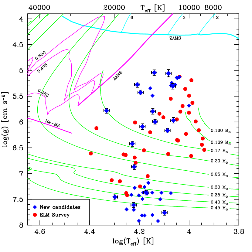
Figure 1.— Surface gravity vs. effective temperature of the 57 WD candidates (blue diamonds) and the previously published ELM Survey WDs (red circles). The 17 newly discovered binaries are plotted with errorbars and parameters obtained from Gianninas stellar atmosphere models; the parameters of the other WDs were obtained from Koester models. For reference, we plot theoretical tracks for 0.16–0.45 $M_{\odot}$ hydrogen atmosphere WDs (green lines, Panei et al., 2007), main sequence tracks for 2, 3 and 6 $M_{\odot}$ stars (cyan lines, Girardi et al., 2004), and horizontal branch tracks for 0.488, 0.495, and 0.500 $M_{\odot}$ stars (magenta lines, Dorman et al., 1993). Zero-age main sequence (ZAMS) and zero-age horizontal branch (ZAHB) isochrones are drawn with thick lines, as is the homogenous helium-burning main sequence (He-MS) from Paczyński (1971).

2.2. New Spectroscopic Observations

We obtain follow-up spectra for each of the candidate low mass WDs to improve stellar atmosphere parameters and to search for velocity variability.

Observations were obtained over the course of seven observing runs at the 6.5m MMT telescope between March 2011 and February 2013. We used the Blue Channel spectrograph (Schmidt et al., 1989) with the 832 line mm^-1 grating, which provides a wavelength coverage 3650 Å to 4500 Å and a spectral resolution of 1.0 Å. All observations were paired with a comparison lamp exposure, and were flux-calibrated using blue spectrophotometric standards (Massey et al., 1988). The extracted spectra typically have a signal-to-noise (S/N) of 7 per pixel in the continuum and a 14 km s^-1 radial velocity error.

We obtained additional spectroscopy for $g<17$ mag ELM WD candidates in queue scheduled time at the 1.5m FLWO telescope. We used the FAST spectrograph (Fabricant et al., 1998) with the 600 line mm^-1 grating and a 1.5″ slit, providing wavelength coverage 3500 Å to 5500 Å and a spectral resolution of 1.7 Å. All observations were paired with a comparison lamp exposure, and were flux-calibrated using blue spectrophotometric standards. The extracted spectra typically have a S/N of 10 per pixel in the continuum and a 18 km s^-1 radial velocity error.

2.3. ELM WD Identifications

Our follow-up observations provide improved stellar atmosphere constraints, from which we determine that 24 (42%) of the candidates are probable ELM WDs with $5<\log{g}<7$ (see Figure 1). The remaining candidates have either $\log{g}>7$ and are normal DA WDs, or $\log{g}\leq 5$ and are presumably halo blue horizontal branch or blue straggler stars.

Figure 1 plots the distribution of $T_{\rm eff}$ vs. $\log{g}$ for all of the WDs with $\log{g}>5$. Previously published ELM Survey stars are marked with red circles. The observed WDs overlap tracks based on Panei et al. (2007) models for He-core WDs with hydrogen shell burning ((green lines) Kilic et al., 2010b), but do not overlap main sequence nor horizontal branch evolutionary tracks. For reference, we also plot Girardi et al. (2002, 2004) solar metallicity main sequence tracks for 2, 3, and 6 $M_{\odot}$ stars (cyan lines). A helium-burning horizontal branch star can have a surface gravity similar to a degenerate He WD (e.g., Heber et al., 2003), but only at a systematically higher effective temperature than that targeted by the ELM Survey. This is illustrated by Dorman et al. (1993) [Fe/H]=-1.48 horizontal branch tracks for 0.488, 0.495, and 0.500 $M_{\odot}$ stars (magenta lines), as well as the homogenous helium-burning main sequence from Paczyński (1971). The zero-age main sequence and helium-burning horizontal branch isochrones (thick lines) mark the limits.

Seventeen of the WDs show significant velocity variability, including twelve of the newly identified ELM WDs. The other ELM WDs have insufficient coverage for detecting (or ruling out) velocity variability. We focus the remainder of this paper on the 17 well-constrained systems.

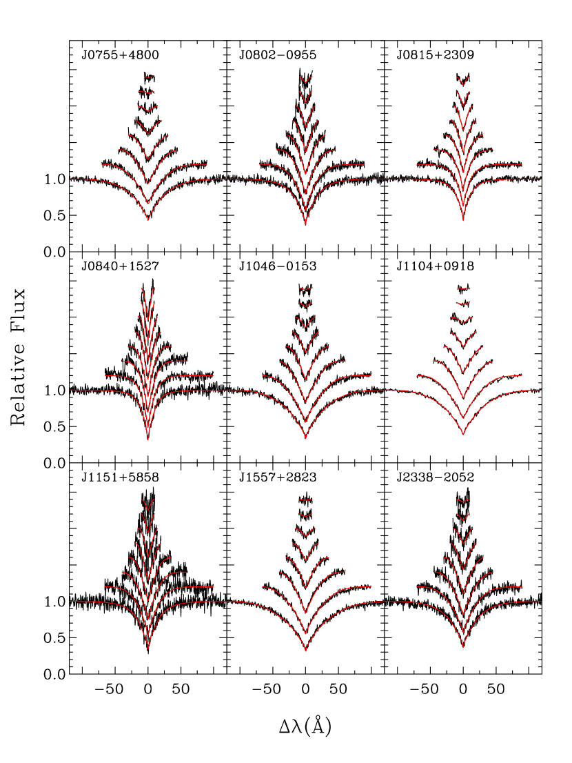
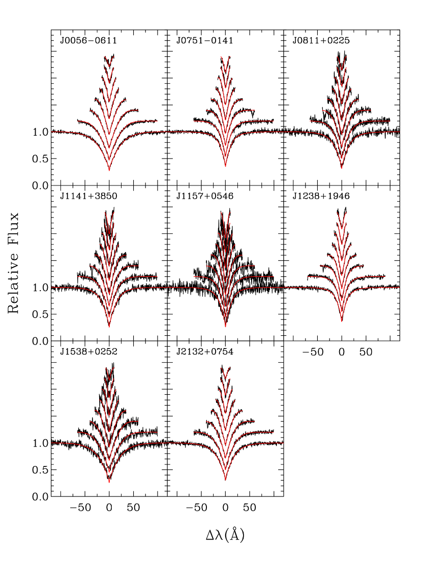
Figure 2.— Gianninas model fits (smooth red lines) overplotted on the composite observed spectra (black lines) for the 17 WD binaries. The Balmer lines are arranged from H12 (top) to H$\gamma$ (bottom); left panel plots the $K<200$ km s^-1 binaries, right panel plots the $K>200$ km s^-1 binaries.

2.4. Improved Atmosphere Parameters

Our sample of 17 well-constrained systems contains four $\log{g}$ $\simeq 5$ objects, objects at the edge of our stellar atmosphere grid that might not be considered degenerate WDs if not for their observed orbital motion. We also fit these stars to grids of Kurucz (1993) models spanning $-4\leq{\rm[Fe/H]}\leq 0.5$, $1\leq\log{g}\leq 5$ (see Allende Prieto et al., 2008) but found very poor solutions. This motivated us to perform a new set of stellar atmosphere fits using Gianninas et al. (2011) hydrogen model atmospheres. The Gianninas models employ improved Stark broadening profiles (Tremblay & Bergeron, 2009), and the ML2/$\alpha$ = 0.8 prescription of the mixing-length theory for models where convective energy transport is important (Tremblay et al., 2010). We calculate atmosphere models for low surface gravities, and use a grid that covers $T_{\rm eff}$ from 4000 K to 30,000 K in steps ranging from 250 to 5000 K and $\log{g}$ from 5.0 to 8.0 in steps of 0.25 dex.

Table 1White Dwarf Physical Parameters

Object	RA	Dec	$T_{\rm eff}$	$\log g$	Mass	$g_{0}$	$M_{g}$	$d_{helio}$
	(h:m:s)	(d:m:s)	(K)	(cm s-2)	($M_{\odot}$)	(mag)	(mag)	(kpc)
J0056$-$0611	0:56:48.232	-6:11:41.62	$12210\pm 180$	$6.167\pm 0.044$	0.17	$17.208\pm 0.023$	8.0	0.69
J0751$-$0141	7:51:41.179	-1:41:20.90	$15660\pm 240$	$5.429\pm 0.046$	0.17	$17.376\pm 0.015$	8.0	0.75
J0755$+$4800	7:55:19.483	48:00:34.07	$19890\pm 350$	$7.455\pm 0.057$	0.42	$15.878\pm 0.019$	9.7	0.18
J0802$-$0955	8:02:50.134	-9:55:49.84	$16910\pm 280$	$6.423\pm 0.048$	0.20	$18.604\pm 0.012$	8.2	1.19
J0811$+$0225	8:11:33.560	2:25:56.76	$13990\pm 230$	$5.794\pm 0.054$	0.17	$18.569\pm 0.013$	8.0	1.30
J0815$+$2309	8:15:44.242	23:09:04.92	$21470\pm 340$	$5.783\pm 0.046$	0.17	$17.623\pm 0.015$	6.7	1.53
J0840$+$1527	8:40:37.574	15:27:04.53	$13810\pm 240$	$5.043\pm 0.053$	0.17	$19.141\pm 0.018$	8.0	1.69
J1046$-$0153	10:46:07.875	-1:53:58.48	$14880\pm 230$	$7.370\pm 0.045$	0.37	$17.927\pm 0.020$	10.2	0.36
J1104$+$0918	11:04:36.739	9:18:22.74	$16710\pm 250$	$7.611\pm 0.049$	0.46	$16.543\pm 0.016$	10.3	0.18
J1141$+$3850	11:41:55.560	38:50:03.02	$11620\pm 200$	$5.307\pm 0.054$	0.17	$18.972\pm 0.018$	8.0	1.56
J1151$+$5858	11:51:38.381	58:58:53.22	$15400\pm 300$	$6.092\pm 0.057$	0.17	$20.046\pm 0.033$	8.0	2.57
J1157$+$0546	11:57:34.455	5:46:45.58	$12100\pm 250$	$5.054\pm 0.071$	0.17	$19.798\pm 0.021$	8.0	2.29
J1238$+$1946	12:38:00.096	19:46:31.45	$16170\pm 260$	$5.275\pm 0.051$	0.17	$17.155\pm 0.019$	8.0	0.68
J1538$+$0252	15:38:44.220	2:52:09.49	$11560\pm 220$	$5.967\pm 0.053$	0.17	$18.528\pm 0.015$	8.0	1.28
J1557$+$2823	15:57:08.483	28:23:36.02	$12550\pm 200$	$7.762\pm 0.046$	0.49	$17.496\pm 0.029$	11.2	0.18
J2132$+$0754	21:32:28.360	7:54:28.24	$13700\pm 210$	$5.995\pm 0.045$	0.17	$17.904\pm 0.019$	8.0	0.96
J2338$-$2052	23:38:21.505	-20:52:22.76	$16630\pm 280$	$6.869\pm 0.050$	0.27	$19.577\pm 0.035$	9.0	1.29

Table 2Binary Orbital Parameters

Object	$N_{obs}$	$P$	$K$	$\gamma$	Spec. Conjunction	$M_{2}$	$q$	$\tau_{\rm merge}$
		(days)	(km s-1)	(km s-1)	HJD-2450000 (days)	($M_{\odot}$)		(Gyr)
J0056$-$0611	33	$0.04338\pm 0.00002$	$376.9\pm 2.4$	$4.2\pm 1.8$	$5864.76305\pm 0.00008$	$\geq$0.45	$\leq$0.374	$\leq$0.12
J0751$-$0141	31	$0.08001\pm 0.00279$	$432.6\pm 2.3$	$61.9\pm 1.8$	$5623.60639\pm 0.00013$	$\geq$0.94	$\leq$0.182	$\leq$0.37
J0755$+$4800	26	$0.54627\pm 0.00522$	$194.5\pm 5.5$	$42.6\pm 3.8$	$3730.89702\pm 0.00208$	$\geq$0.90	$\leq$0.468	$\leq$28
J0802$-$0955	20	$0.54687\pm 0.00455$	$176.5\pm 4.5$	$27.0\pm 3.4$	$5623.34011\pm 0.00228$	$\geq$0.57	$\leq$0.348	$\leq$79
J0811$+$0225	24	$0.82194\pm 0.00049$	$220.7\pm 2.5$	$77.4\pm 1.9$	$6329.61559\pm 0.00296$	$\geq$1.20	$\leq$0.142	$\leq$160
J0815$+$2309	21	$1.07357\pm 0.00018$	$131.7\pm 2.6$	$-37.0\pm 2.6$	$5623.68831\pm 0.00415$	$\geq$0.47	$\leq$0.361	$\leq$620
J0840$+$1527	19	$0.52155\pm 0.00474$	$84.8\pm 3.1$	$10.7\pm 2.3$	$4822.83144\pm 0.00244$	$\geq$0.15	$\leq$0.879	$\leq$230
J1046$-$0153	16	$0.39539\pm 0.10836$	$80.8\pm 6.6$	$-33.3\pm 4.6$	$4597.54154\pm 0.00293$	$\geq$0.19	$\leq$0.509	$\leq$48
J1104$+$0918	25	$0.55319\pm 0.00502$	$142.1\pm 6.0$	$72.5\pm 4.0$	$3793.84175\pm 0.00269$	$\geq$0.55	$\leq$0.831	$\leq$39
J1141$+$3850	17	$0.25958\pm 0.00005$	$265.8\pm 3.5$	$-11.2\pm 2.2$	$3881.73870\pm 0.00037$	$\geq$0.76	$\leq$0.225	$\leq$10
J1151$+$5858	17	$0.66902\pm 0.00070$	$175.7\pm 5.9$	$12.0\pm 4.2$	$5622.52148\pm 0.00269$	$\geq$0.61	$\leq$0.277	$\leq$150
J1157$+$0546	9	$0.56500\pm 0.01925$	$158.3\pm 4.9$	$-124.8\pm 3.3$	$4235.73743\pm 0.00244$	$\geq$0.44	$\leq$0.382	$\leq$120
J1238$+$1946	21	$0.22275\pm 0.00009$	$258.6\pm 2.5$	$-6.6\pm 1.2$	$4236.71749\pm 0.00032$	$\geq$0.64	$\leq$0.266	$\leq$7.5
J1538$+$0252	16	$0.41915\pm 0.00295$	$227.6\pm 4.9$	$-157.9\pm 3.9$	$5385.57030\pm 0.00146$	$\geq$0.76	$\leq$0.222	$\leq$35
J1557$+$2823	24	$0.40741\pm 0.00294$	$131.2\pm 4.2$	$10.4\pm 3.0$	$3563.72487\pm 0.00127$	$\geq$0.43	$\leq$0.886	$\leq$20
J2132$+$0754	35	$0.25056\pm 0.00002$	$297.3\pm 3.0$	$-12.1\pm 2.0$	$5862.68632\pm 0.00049$	$\geq$0.95	$\leq$0.179	$\leq$7.7
J2338$-$2052	25	$0.07644\pm 0.00712$	$133.4\pm 7.5$	$5.2\pm 4.8$	$5862.75190\pm 0.00049$	$\geq$0.15	$\leq$0.554	$\leq$0.95

Note. — Objects with significant period aliases: J0755+4800 (0.349 days), J0840+1527 (0.340 days), J1046$-$0153 (0.659 days), J1104+0918 (0.355 days), J1157+0546 (1.23 days), J1538+0252 (0.295 days), and J1557+2823 (0.677 and 0.290 days) as seen in Figure 3.

Our stellar atmosphere fits use the so-called spectroscopic technique described in Gianninas et al. (2011). One difference between our work and Gianninas et al. (2011) is that we fit higher-order Balmer lines, up to and including H12, observed in the low surface gravity ELM WDs. The higher-order Balmer lines are sensitive to $\log{g}$ and improve our surface gravity measurement. For the handful of WDs in our sample with $\log{g}>7$, we only fit Balmer lines up to and including H10 since the higher order Balmer lines are not observed at higher surface gravity.

The lowest gravity WDs in our sample show Ca and Mg lines in their spectra. For reference, the diffusion timescale for Ca in a $T_{\rm eff}=$ 10,000 K, 0.2 $M_{\odot}$ H-rich WD is $\sim$$10^{4}$ yr (Paquette et al., 1986). Extreme horizontal branch stars, which can have surface gravities comparable to the lowest gravity WDs, have longer $\sim$$10^{6}$ yr diffusion timescales (Michaud et al., 2008). These diffusion timescales are shorter than the WD evolutionary timescale, suggesting there may be on-going accretion in these ultra-compact binary systems. Near- and mid-infrared observations are needed constrain the possibility of accretion. We defer a detailed analysis of the metal abundances in ELM WDs to a future paper. For our present analysis we exclude the wavelength ranges where the metal lines are present in our fits.

Our error estimates combine the internal error of the model fits, obtained from the covariance matrix of the fitting algorithm, and the external error, obtained from multiple observations of the same object. Uncertainties are typically 1.2% in $T_{\rm eff}$ and 0.038 dex in $\log{g}$ (see Liebert et al., 2005, for details). A measure of the systematic uncertainty inherent in the stellar atmosphere models and fitting routines comes from Gianninas et al. (2011), who find a systematic uncertainty of $\approx 0.1$ dex in $\log{g}$. This is corroborated by the difference we observe between the different fitting methods discussed in Section 2.1 and here: the mean difference and the dispersion in $T_{\rm eff}$is $1.1\%\pm 4.3\%$ and in $\log{g}$is $0.05\pm 0.12$ dex. Figure 1 plots the properties of the 17 WDs with their internal errorbars.

We use Panei et al. (2007) evolutionary tracks to estimate WD mass and luminosity. For purpose of discussion, we assume $\log{g}<6$ WDs have mass 0.17 $M_{\odot}$ and absolute magnitude $M_{g}=8.0$ (see Kilic et al., 2011a; Vennes et al., 2011). We summarize the observed and derived stellar parameters of the 17 new binaries in Table 1. Position and de-reddened $g$-band magnitude come from SDSS (Aihara et al., 2011) and $d_{helio}$ is our heliocentric distance estimate.

Figure 3.— Periodograms for the 17 WD binaries. The best orbital periods have the smallest $\chi^{2}$ values; some binaries are well constrained and some have period aliases.

Figure 4.— Observed velocities phased to best-fit orbits for the 17 WD binaries (Table 2).

2.5. Orbital Elements

We calculate orbital elements and merger times in the same way as previous ELM Survey papers, and so we refer the reader to those papers for the details of our analysis. In brief, we measure absolute radial velocities using the cross-correlation package RVSAO (Kurtz & Mink, 1998) and a high-S/N template. We use the entire spectrum in the cross-correlation. We then use the summed spectra (Figure 2) as cross-correlation templates to maximize our velocity precision for each individual object. We calculate orbital elements by minimizing $\chi^{2}$ for a circular orbit using the code of Kenyon & Garcia (1986). Figure 3 shows the periodograms for the 17 binaries, and Figure 4 plots the radial velocities phased to the best-fit orbital periods. We use the binary mass function to estimate the unseen companion mass; an edge-on orbit with inclination $i=90\arcdeg$ yields the minimum companion mass $M_{2}$ and the maximum gravitational wave merger time.

Table 2 summarizes the binary orbital parameters. Columns include orbital period ($P$), radial velocity semi-amplitude ($K$), systemic velocity ($\gamma$), time of spectroscopic conjunction (the time when the object is closest to us), minimum secondary mass ($M_{2}$) assuming $i=90\arcdeg$, the maximum mass ratio ($q$), and the maximum gravitational wave merger time $\tau_{\rm merge}$. The systemic velocities in Table 2 are not corrected for the WDs’ gravitational redshifts, which should be subtracted from the observed velocities to find the true systemic velocities. This correction is a few km s^-1 for a 0.17 $M_{\odot}$ helium WD, comparable to the systemic velocity uncertainty.

3. RESULTS

The orbital solutions constrain the nature of the ELM WD binaries. Here we discuss the systems with short merger times, massive companions, or that may be underluminous supernovae progenitors.

3.1. J0056$-$0611

The ELM WD J0056$-$0611 has a well-constrained orbital period of $1.0409\pm 0.0005$ hr and a semi-amplitude of $377\pm 2$ km s^-1. We can calculate its likely companion mass if we assume a distribution for the unknown orbital inclination. Although radial velocity detections are biased towards edge-on systems (see Section 4), we will assume that we are observing a random inclination for purpose of discussion. The mean inclination angle for a random sample, $i=60\arcdeg$, is then an estimate of the most likely companion mass. For J0056$-$0611, the most likely companion is a 0.61 $M_{\odot}$ WD at an orbital separation of 0.5 $R_{\odot}$. This orbital separation rules out the possibility of a main sequence companion.

There is no evidence for a 0.61 $M_{\odot}$ WD in the spectrum of J0056$-$0611, but we would not expect there to be. If the two WDs in this binary formed at the same time, we would expect the 0.61 $M_{\odot}$ WD to be 15 - 100 times less luminous than the 0.17 $M_{\odot}$ WD for cooling ages of 100 Myr - 1 Gyr (Bergeron et al., 1995). A more plausible evolutionary scenario for an ELM WD binary like J0056$-$0611 is two consecutive phases of common-envelope evolution in which the ELM WD is created last, giving the more massive WD a longer time to cool and fade (e.g. Kilic et al., 2007b).

For the most probable companion mass of 0.61 $M_{\odot}$, J0056$-$0611 will begin mass transfer in 100 Myr. Kilic et al. (2010b) discuss the many possible stellar evolution paths for such a system. This system’s mass ratio $q\leq$0.37 suggests that mass transfer will likely be stable (Marsh et al., 2004) and that J0056$-$0611 will evolve into an AM CVn system.

3.2. J0751$-$0141

The ELM WD J0751$-$0141 has a $1.920\pm 0.067$ hr orbital period with aliases ranging between 1.85 and 2.05 hr (see Figure 3). The large $433\pm 2$ km s^-1 semi-amplitude indicates that the companion is massive, regardless of the exact period. The minimum companion mass is 0.94 $M_{\odot}$. Assuming a random inclination distribution, there is a 47% probability that the companion is $>$1.4 $M_{\odot}$.

Given that the ELM WD went through a common envelope phase of evolution with its companion, J0751$-$0141 possibly contains a milli-second pulsar binary companion. Helium-core WDs are the most common type of companion in known milli-second pulsar binaries (Tauris et al., 2012). We have been allocated Cycle 14 Chandra X-ray Observatory time to search for X-ray emission from a possible neutron star.

For $i=60\arcdeg$, the companion is a 1.32 $M_{\odot}$ WD, and the system will begin mass transfer in 290 Myr. The extreme mass ratio $q\leq$0.18 means that this system will undergo stable mass transfer and evolve into an AM CVn system. As the binary orbit widens in the AM CVn phase, the mass accretion rate will drop and the mass required for the unstable burning of the accreted He-layer increases up to several percent of a solar mass. The final flash should ignite a thermonuclear transient visible as an underluminous supernova (Bildsten et al., 2007; Shen & Bildsten, 2009). It is also possible that the helium flash will detonate the massive WD in a double-detonation scenario (Sim et al., 2012, though see Dan et al. 2012). If J0751$-$0141 has a massive WD companion, it is a probable supernova progenitor.

3.3. J0811+0225

The ELM WD J0811+0225 has an orbital period of $19.727\pm 0.012$ hr and a semi-amplitude of 221 km s^-1. These orbital parameters yield a minimum companion mass of 1.20 $M_{\odot}$. That means the companion probably exceeds a Chandrasekhar mass. For $i=60\arcdeg$, the most likely companion is a 1.70 $M_{\odot}$ neutron star at an orbital separation of 4.6 $R_{\odot}$. There is no Fermi gamma-ray detection at this location, but additional observations are needed to determine the nature of this system.

3.4. J0840+1527

The ELM WD J0840+1527 has a best-fit $\log{g}$$=5.043\pm 0.053$ near the limit of our model grid. Its best-fit orbital period is $12.517\pm 0.114$ hr with a significant alias at 8.3 hr. Assuming this object is 0.17 $M_{\odot}$, its most likely companion is a WD with a comparable mass, 0.19 $M_{\odot}$, at an orbital separation of 1.9 $R_{\odot}$. If, on the other hand, J0840+1527 were a 3 $M_{\odot}$ main sequence star, its companion would have an orbital separation of 4.3 $R_{\odot}$ – a separation comparable to the radius of a 3 $M_{\odot}$ star, and thus physically implausible. There is no evidence for mass transfer in this system. We conclude that J0840+1527 is a pair of ELM WDs.

3.5. J1141+3850, J1157+0546, and J1238+1946

J1141+3850, J1157+0546, and J1238+1946 are the other systems containing WDs near the low-gravity limit of our stellar atmosphere model grid, but their $k=158$ - 266 km s^-1 semi-amplitudes are significantly larger than that of J0840+1527. If we assume that the objects are 0.17 $M_{\odot}$ ELM WDs, then the binary companions have minimum masses of 0.45 - 0.75 $M_{\odot}$. If we instead assume that the objects are main sequence stars, then the required orbital separations are comparable to the radius of the main sequence star and physically impossible. There is no evidence for mass transfer in these systems.

We conclude that J1141+3850, J1157+0546, and J1238+1946 are ELM WDs with likely WD companions. For J1141+3850, there is a 36% probability that the companion is $>$1.4 $M_{\odot}$, possibly a milli-second pulsar. For J1141+3850 and J1238+1946, mass transfer will begin in 7-10 Gyr, making them AM CVn progenitors and possible underluminous supernovae progenitors.

3.6. J2132+0754

The ELM WD J2132+0754 has a well-constrained orbital period of $6.0134\pm 0.0004$ hr and semi-amplitude of $297\pm 3$ km s^-1. The minimum companion mass is 0.95 $M_{\odot}$, and there is a 48% probability that the companion is $>$1.4 $M_{\odot}$, possibly a milli-second pulsar. For $i=60\arcdeg$, the most likely companion is a 1.33 $M_{\odot}$ WD that will begin mass transfer in 6 Gyr. That makes J2132+0754 a likely AM CVn progenitor and another possible underluminous supernovae progenitor.

3.7. J2338$-$2052

The ELM WD J2338$-$2052 has an orbital period of $1.834\pm 0.170$ hr and a semi-amplitude of $133\pm 7$ km s^-1. In this case the companion is another ELM WD; for $i=60\arcdeg$, the most likely companion is a 0.17 $M_{\odot}$ WD at an orbital separation of 0.56 $R_{\odot}$. Given the unity mass ratio, this system will undergo unstable mass transfer and will merge to form a single $\sim$0.4 $M_{\odot}$ WD. This system will merge in less than 1 Gyr.

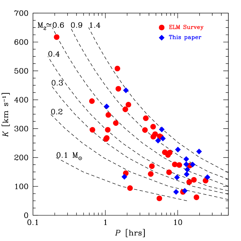
Figure 5.— Orbital period vs. semi-amplitude for the ELM Survey binaries. Previously published binaries are drawn with solid red circles; the 17 binaries from this paper are drawn with solid blue diamonds. Dashed lines indicate approximate companion mass under the assumption that $M_{1}=0.2$ $M_{\odot}$ and $i=60\arcdeg$.

4. DISCUSSION

With these 17 new discoveries, plus the pulsating ELM WD discovery published by Hermes et al. (2013), the ELM Survey has found 54 detached, double degenerate binaries; 31 of the binaries will merge within a Hubble time. Table 5 summarizes the properties of the systems. Eighty percent of the ELM Survey binaries are formally ELM WD systems.

4.1. Significance of Binary Detections

We find low mass WDs in compact binaries, binaries that must have gone through common envelope evolution. This makes sense because extremely low mass WDs require significant mass loss to form; the Universe is not old enough to produce an extremely low mass WD through single star evolution. Yet four objects published in the ELM Survey have no significant velocity variability, two of which are ELM WDs (see Table 5). To understand whether or not these stars are single requires that we understand the significance of our binary detections.

Each ELM Survey binary is typically constrained by 10-30 irregularly spaced velocities with modest errors. Given that we determine orbital parameters by minimizing $\chi^{2}$, the $F$-test is a natural choice. We use the $F$-test to check whether the variance of the data around the orbital fit is consistent with the variance of the data around a constant velocity (we use the weighted mean of the observations). $F$-test probabilities for the published ELM Survey binaries are $<0.01$. In other words, our binaries have significant velocity variability at the $>99$% confidence level.

In the null cases we need to calculate the likelihood of not detecting a binary. This is a trickier problem, and one that we approach with a Monte Carlo calculation. We start by selecting a set of observations (times, velocity errors) and an orbital period and semi-amplitude. We convert observation times to orbital phases using a randomly drawn zero time, and calculate velocities at those phases summed with a randomly drawn velocity error. We perform the $F$-test, using 0.01 as a detection threshold. We repeat this calculation 10,000 times for a given orbital period and semi-amplitude, and then select a new orbital period and semi-amplitude to iterate on. This analysis is done for each object.

We find that the datasets for our 17 new binaries have a median 99.9% likelihood of detecting $K=200$ km s^-1 binaries, a 97% likelihood of detecting $K=100$ km s^-1 binaries, and a 44% likelihood of detecting $K=50$ km s^-1 binaries. It is no surprise that we are less likely to detect a low semi-amplitude binary, but this analysis suggests that we can be quite confident of detecting $K>100$ km s^-1 systems. We find very similar likelihoods for detecting binaries containing ELM WDs in the full ELM Survey sample.

The datasets for the null cases typically contain fewer observations and so are not as well-constrained. For J0900+0234, a 0.16 $M_{\odot}$ ELM WD with no observed velocity variation (Brown et al., 2012b), the likelihoods of detecting a $K=200$, 100, and 50 km s^-1 binary are 87%, 57%, and 10%, respectively. Additional observations are required to claim this ELM WD as non-variable.

There is, of course, an orbital period dependence to the detections, and periods near 24 hr are the most problematic. Taken together, our datasets have a median 39% likelihood of detecting a $K=100$ km s^-1 binary at $P=24$ hr. Yet we remain sensitive to longer periods: our datasets have median 99% and 98% likelihoods of detecting a $K=100$ km s^-1 binary at $P=18$ hr and $P=36$ hr, respectively.

Figure 5 plots the observed distribution of $P$ and $K$ for the ELM Survey binaries. The dashed lines indicate the approximate companion mass assuming $M_{1}$ is 0.2 $M_{\odot}$ and $i$ is 60$\arcdeg$. At $K=100$ km s^-1, we can detect companion masses down to 0.1 $M_{\odot}$ at 2 hr orbital periods and 0.55 $M_{\odot}$ companions at 2 day orbital periods. Systems with $K<100$ km s^-1 are the realm of $\lesssim$0.2 $M_{\odot}$ companions, and we observe a half-dozen systems with these parameters. Our incompleteness at $K<100$ km s^-1 implies there are quite likely more ELM WDs with $\simeq$0.2 $M_{\odot}$ companions; the remaining ELM WD candidates that do not show obvious velocity change in a couple observations are possible examples of such low amplitude systems.

Finally, orbital inclination acts to increase the difficulty of identifying lone ELM WDs. Consider the set of 46 ELM WDs in Table 5 with $\log{g}<7$, two of which are non-variable. Their median $K$ is 240 km s^-1, a semi-amplitude that would appear $<50$ km s^-1 at $i<12\arcdeg$. If the 46 objects have randomly distributed orbital inclinations, one object should have $i<12\arcdeg$ and a second $i<17\arcdeg$. We conclude there is no good evidence for a lone ELM WD in our present sample. This is in stark contrast to the population of 0.4 $M_{\odot}$ WDs in the solar neighborhood, of which 20%-30% are single (Brown et al., 2011a).

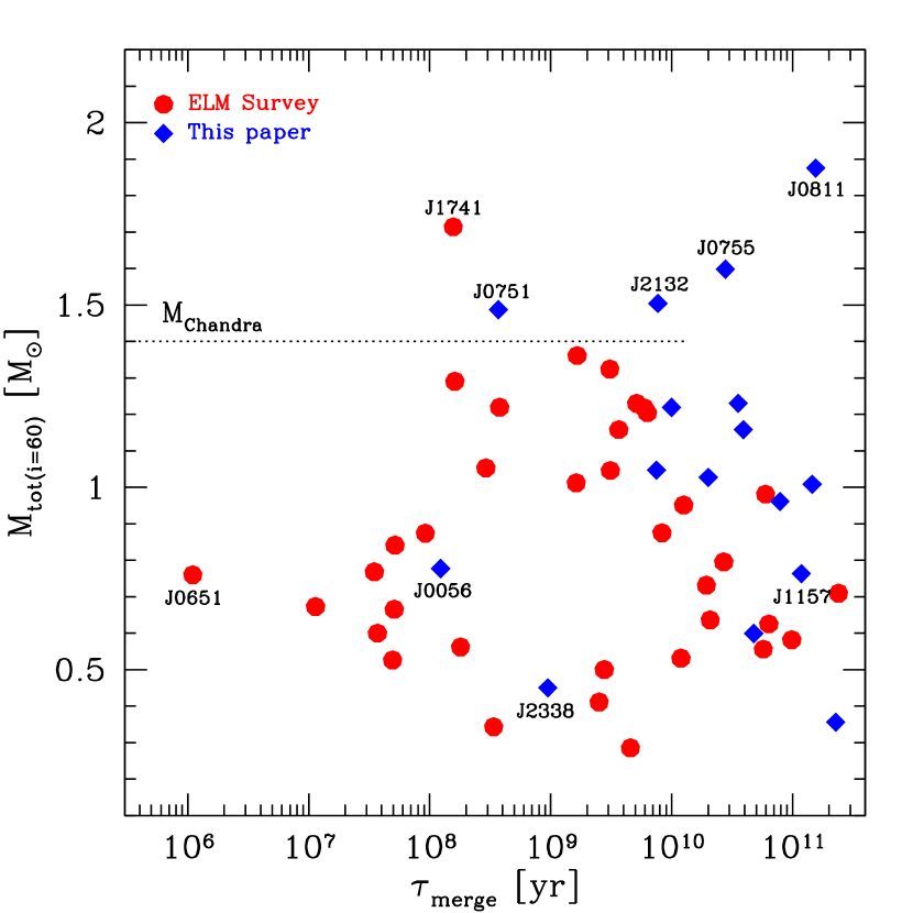
Figure 6.— Gravitational wave merger time versus total system mass for the ELM Survey. We calculate system mass assuming $i=60^{\arcdeg}$ when orbital inclination is unknown. Previously published ELM Survey binaries are drawn with solid red circles, and the 17 new binaries from this paper are drawn with solid blue diamonds. Six binaries have probable masses exceeding the Chandrasekhar mass; three have merger times less than 10 Gyr, as indicated by the dotted line. The minimum companion mass for J0811+0225 is 1.2 $M_{\odot}$.

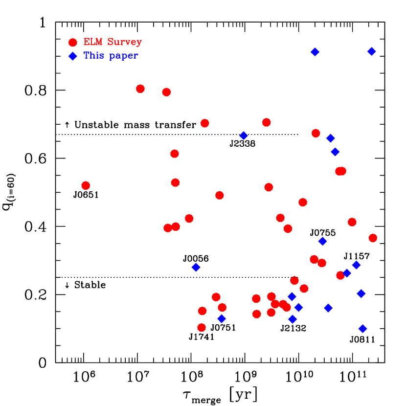
Figure 7.— Gravitational wave merger time versus mass ratio $q$ for the ELM Survey. We calculate mass ratio assuming $i=60^{\arcdeg}$ when orbital inclination is unknown. Previously published ELM Survey binaries are drawn with solid red circles, and the 17 new binaries from this paper are drawn with solid blue diamonds. Dotted lines mark the approximate thresholds for stability of mass transfer during the Roche lobe overflow phase (Marsh et al., 2004), drawn for systems that will merge in $<$10 Gyr. Stable mass transfer systems will evolve into AM CVn systems; unstable mass transfer systems will possibly merge.

4.2. The Future of ELM WDs

One of the most exciting aspects of our ELM WD binaries is that many have gravitational wave merger times less than a Hubble time, and in one case as short as 1 Myr (Brown et al., 2011c; Hermes et al., 2012b). A natural question, then, is what will happen when the WDs merge. Notably, 5 of our 17 new binaries have probable system masses (for $i=60\arcdeg$) in excess of a Chandrasekhar mass.

Figure 6 plots the distribution of merger time and system mass for the ELM Survey binaries assuming $i=60\arcdeg$, except when inclination is known. The majority of our binaries have probable masses below the Chandrasekhar mass and are not potential supernova Type Ia progenitors, but six systems appear to have either neutron star or massive WD companions. The evolution of these six systems depends on the stability of mass transfer during the Roche lobe overflow phase, and thus on the mass ratio of the binary.

Figure 7 plots the distribution of merger time and mass ratio $q$ for the ELM Survey binaries, again assuming $i=60\arcdeg$ except when inclination is known. The Chandrasekhar mass systems generally have extreme $q\lesssim 0.15$ and so will evolve into stable mass transfer AM CVn systems. If the accretors are massive WDs, these systems should experience a large helium flash that may appear as an underluminous .Ia supernova (e.g. Bildsten et al., 2007; Shen & Bildsten, 2009). It is also possible that the helium flash will detonate the massive WD in a double-detonation scenario (Sim et al., 2012). The Chandrasekhar mass systems are thus potential supernovae progenitors. However, the outcome of a merger of an ELM WD with a massive WD is uncertain (see Dan et al., 2012).

Systems with $q\geq 2/3$, such as J2338$-$2052, will experience unstable mass transfer. These systems may merge (Dan et al., 2011) to form a single low-mass WD, R CrB star, or helium-burning sdB star. Systems with intermediate $q\simeq 1/2$, such as J0651+2844, will experience either stable or unstable mass transfer depending on their spin-orbit coupling. After we constrain the remaining ELM WD candidates plotted in Fig. 1 we look forward to calculating their space density and merger rate. ELM WDs binaries are clearly an important channel for AM CVn star formation, and thus an important source of strong gravitational waves in the mHz regime.

5. CONCLUSION

We perform stellar atmosphere fits to the entire collection of single-epoch spectra in the HVS Survey and identify 57 new low mass WD candidates. Follow-up spectroscopy reveals 17 WDs with significant velocity variability, 12 of which are ELM WDs. Presently, the ELM Survey sample is consistent with all of the ELM WDs being part of close binaries. ELM WDs are thus signposts for binaries that are strong gravitational wave sources and possible supernovae progenitors.

Four binaries in our sample contain $\log{g}\simeq 5$ objects, objects that might not be considered WDs or proto-WDs if not for their observed orbital motion. The existence of $\log{g}\simeq 5$ WDs motivates us to develop a new set of stellar atmosphere models following Gianninas et al. (2011). Interestingly, all of the lowest surface gravity ($\log{g}<6$) WDs in our sample have metal lines in their spectra. This issue will be studied in detail in a future paper; infrared observations are needed to constrain the possibility of debris disks as the source of Ca and Mg accretion in these compact binary systems.

Recent discoveries of pulsations in several of our ELM WD targets (Hermes et al., 2012c, 2013) enable us to probe the interiors of low-mass, presumably He-core WDs using the tools of asteroseismology. Due to the HVS color selection, all of the newly identified systems are hotter than 10,000 K and therefore too hot to show the g-mode pulsations detected in cooler ELM WDs (Córsico et al., 2012).

Four binaries in our sample have massive $\gtrsim$0.9 $M_{\odot}$ companions and $<$10 Gyr merger times. If the unseen companions are massive WDs, these extreme mass ratio binaries will undergo stable mass transfer and will evolve into AM CVn systems and potentially future .Ia or underluminous supernovae. Thus the systems J0751$-$0141, J1141+3850, J1238+1946, and J2132+0754 are possible supernova progenitors.

The other possibility is that the massive companions in these four binaries are neutron stars. Given their past common envelope evolution, the systems quite possibly contain milli-second pulsars. A fifth system, J0811+0225, appears to have a minimum companion mass close to a Chandrasekhar mass. We are conducting follow-up optical, radio, and X-ray observations to establish the nature of these extreme mass ratio ELM WD binaries. Optically visible WD companions of neutron stars are useful for constraining the binary mass ratio and also to calibrate the spin-down ages of milli-second pulsars.

Given our present observations, we expect that the ELM Survey will grow to 100 binaries in a few years. A large sample is important for finding more systems like J0651+2844, a 12.75 min period system that provides us with a laboratory for measuring the spin-orbit coupling and tidal heating of a rapidly merging pair of WDs. We expect that photometric observations will discover more pulsating ELM WDs. Finally, a larger sample of ELM WDs will be an important source of gravitational wave verification sources for $eLISA$ and other future gravitational wave detection experiments.

Table 3Merger and Non-Merger Systems in the ELM Survey

Object	$T_{\rm eff}$	$\log{g}$	$P$	$K$	Mass	$M_{2}$	$M_{2}(60\arcdeg)$	$\tau_{\rm merge}$	Ref
	(K)	(cm s-2)	(days)	km s-1	$M_{\odot}$	$M_{\odot}$	$M_{\odot}$	Gyr
J0022$-$1014	18980	7.15	0.07989	145.6	0.33	$\geq 0.19$	0.23	$\leq 0.73$	6
J0056$-$0611	12210	6.17	0.04338	376.9	0.17	$\geq 0.46$	0.61	$\leq 0.12$
J0106$-$1000	16490	6.01	0.02715	395.2	0.17	0.43	$\cdots$	0.037	7
J0112+1835	9690	5.63	0.14698	295.3	0.16	$\geq 0.62$	0.85	$\leq 2.7$	1
J0651+2844	16530	6.76	0.00886	616.9	0.26	0.50	$\cdots$	0.0011	3,15
J0751$-$0141	15660	5.43	0.08001	432.6	0.17	$\geq 0.94$	1.32	$\leq 0.37$
J0755+4906	13160	5.84	0.06302	438.0	0.17	$\geq 0.81$	1.12	$\leq 0.22$	2
J0818+3536	10620	5.69	0.18315	170.0	0.17	$\geq 0.26$	0.33	$\leq 8.9$	2
J0822+2753	8880	6.44	0.24400	271.1	0.17	$\geq 0.76$	1.05	$\leq 8.4$	4
J0825+1152	24830	6.61	0.05819	319.4	0.26	$\geq 0.47$	0.61	$\leq 0.18$	0
J0849+0445	10290	6.23	0.07870	366.9	0.17	$\geq 0.64$	0.88	$\leq 0.47$	4
J0923+3028	18350	6.63	0.04495	296.0	0.23	$\geq 0.34$	0.44	$\leq 0.13$	2
J1005+0542	15740	7.25	0.30560	208.9	0.34	$\geq 0.66$	0.86	$\leq 9.0$	0
J1005+3550	10010	5.82	0.17652	143.0	0.17	$\geq 0.19$	0.24	$\leq 10.3$	0
J1053+5200	15180	6.55	0.04256	264.0	0.20	$\geq 0.26$	0.33	$\leq 0.16$	4,9
J1056+6536	20470	7.13	0.04351	267.5	0.34	$\geq 0.34$	0.43	$\leq 0.085$	0
J1112+1117	9590	6.36	0.17248	116.2	0.17	$\geq 0.14$	0.17	$\leq 12.7$	16
J1141$+$3850	11620	5.31	0.25958	265.8	0.17	$\geq 0.76$	1.05	$\leq 9.96$
J1233+1602	10920	5.12	0.15090	336.0	0.17	$\geq 0.86$	1.20	$\leq 2.1$	2
J1234$-$0228	18000	6.64	0.09143	94.0	0.23	$\geq 0.09$	0.11	$\leq 2.7$	6
J1238$+$1946	16170	5.28	0.22275	258.6	0.17	$\geq 0.64$	0.88	$\leq 7.49$
J1436+5010	16550	6.69	0.04580	347.4	0.24	$\geq 0.46$	0.60	$\leq 0.10$	4,9
J1443+1509	8810	6.32	0.19053	306.7	0.17	$\geq 0.83$	1.15	$\leq 4.1$	1
J1630+4233	14670	7.05	0.02766	295.9	0.30	$\geq 0.30$	0.37	$\leq 0.031$	8
J1741+6526	9790	5.19	0.06111	508.0	0.16	$\geq 1.10$	1.55	$\leq 0.17$	1
J1840+6423	9140	6.16	0.19130	272.0	0.17	$\geq 0.64$	0.88	$\leq 5.0$	1
J2103$-$0027	10000	5.49	0.20308	281.0	0.17	$\geq 0.71$	0.99	$\leq 5.4$	0
J2119$-$0018	10360	5.36	0.08677	383.0	0.17	$\geq 0.75$	1.04	$\leq 0.54$	2
J2132$+$0754	13700	6.00	0.25056	297.3	0.17	$\geq 0.95$	1.33	$\leq 7.70$
J2338$-$2052	16630	6.87	0.07644	133.4	0.27	$\geq 0.15$	0.18	$\leq 0.95$
NLTT11748	8690	6.54	0.23503	273.4	0.18	0.76	$\cdots$	7.2	5,10,11
J0022+0031	17890	7.38	0.49135	80.8	0.38	$\geq 0.21$	0.26	$\cdots$	6
J0152+0749	10840	5.80	0.32288	217.0	0.17	$\geq 0.57$	0.78	$\cdots$	1
J0730+1703	11080	6.36	0.69770	122.8	0.17	$\geq 0.32$	0.41	$\cdots$	0
J0755$+$4800	19890	7.46	0.54627	194.5	0.42	$\geq 0.90$	1.18	$\cdots$
J0802$-$0955	16910	6.42	0.54687	176.5	0.20	$\geq 0.57$	0.76	$\cdots$
J0811$+$0225	13990	5.79	0.82194	220.7	0.17	$\geq 1.20$	1.71	$\cdots$
J0815$+$2309	21470	5.78	1.07357	131.7	0.17	$\geq 0.47$	0.63	$\cdots$
J0840$+$1527	13810	5.04	0.52155	84.8	0.17	$\geq 0.15$	0.19	$\cdots$
J0845+1624	17750	7.42	0.75599	62.2	0.40	$\geq 0.19$	0.22	$\cdots$	0
J0900+0234	8220	5.78	$\cdots$	$\leq 24$	0.16	$\cdots$	$\cdots$	$\cdots$	1
J0917+4638	11850	5.55	0.31642	148.8	0.17	$\geq 0.28$	0.36	$\cdots$	12
J1046$-$0153	14880	7.37	0.39539	80.8	0.37	$\geq 0.19$	0.23	$\cdots$
J1104$+$0918	16710	7.61	0.55319	142.1	0.46	$\geq 0.55$	0.70	$\cdots$
J1151$+$5858	15400	6.09	0.66902	175.7	0.17	$\geq 0.61$	0.84	$\cdots$
J1157$+$0546	12100	5.05	0.56500	158.3	0.17	$\geq 0.45$	0.59	$\cdots$
J1422+4352	12690	5.91	0.37930	176.0	0.17	$\geq 0.41$	0.55	$\cdots$	2
J1439+1002	14340	6.20	0.43741	174.0	0.18	$\geq 0.46$	0.62	$\cdots$	2
J1448+1342	12580	6.91	$\cdots$	$\leq 35$	0.25	$\cdots$	$\cdots$	$\cdots$	2
J1512+2615	12130	6.62	0.59999	115.0	0.20	$\geq 0.28$	0.36	$\cdots$	2
J1518+0658	9810	6.66	0.60935	172.0	0.20	$\geq 0.58$	0.78	$\cdots$	1
J1538$+$0252	11560	5.97	0.41915	227.6	0.17	$\geq 0.77$	1.06	$\cdots$
J1557$+$2823	12550	7.76	0.40741	131.2	0.49	$\geq 0.43$	0.54	$\cdots$
J1625+3632	23570	6.12	0.23238	58.4	0.20	$\geq 0.07$	0.08	$\cdots$	6
J1630+2712	11200	5.95	0.27646	218.0	0.17	$\geq 0.52$	0.70	$\cdots$	2
J2252$-$0056	19450	7.00	$\cdots$	$\leq 25$	0.31	$\cdots$	$\cdots$	$\cdots$	2
J2345$-$0102	33130	7.20	$\cdots$	$\leq 43$	0.42	$\cdots$	$\cdots$	$\cdots$	2
LP400$-$22	11170	6.35	1.01016	119.9	0.19	$\geq 0.41$	0.52	$\cdots$	13,14

References. — (0) Kilic et al. (2012); (1) Brown et al. (2012b); (2) Brown et al. (2010); (3) Brown et al. (2011c); (4) Kilic et al. (2010b); (5) Kilic et al. (2010a); (6) Kilic et al. (2011a); (7) Kilic et al. (2011c); (8) Kilic et al. (2011b); (9) Mullally et al. (2009); (10) Steinfadt et al. (2010); (11) Kawka et al. (2010); (12) Kilic et al. (2007a); (13) Kilic et al. (2009); (14) Vennes et al. (2009) ; (15) Hermes et al. (2012b) ; (16) Hermes et al. (2013)

Appendix A DATA TABLE

Table 4 presents our radial velocity measurements. The Table columns include object name, heliocentric Julian date (based on UTC), heliocentric radial velocity (uncorrected for the WD gravitational redshift), and velocity error.

Table 4Radial Velocity Measurements

Object	HJD	$v_{helio}$
	(days$-$2450000)	(km s-1)
J0056$-$0611	5864.778351	$308.7\pm 9.7$
$\cdots$	5864.786174	$-64.5\pm 9.5$
$\cdots$	5864.788281	$-162.4\pm 10.7$
$\cdots$	5864.789600	$-249.1\pm 8.8$
$\cdots$	5864.790804	$-258.9\pm 10.8$
$\cdots$	5864.792007	$-304.9\pm 10.3$

Note. — (This table is available in its entirety in machine-readable and Virtual Observatory forms in the online journal. A portion is shown here for guidance regarding its form and content.)

References

- Aihara et al. (2011) Aihara, H., Allende Prieto, C., An, D., et al. 2011, ApJS, 193, 29
- Allende Prieto et al. (2006) Allende Prieto, C., Beers, T. C., Wilhelm, R., et al. 2006, ApJ, 636, 804
- Allende Prieto et al. (2008) Allende Prieto, C., Sivarani, T., Beers, T. C., et al. 2008, AJ, 136, 2070
- Bassa et al. (2006) Bassa, C. G., van Kerkwijk, M. H., Koester, D., & Verbunt, F. 2006, A&A, 456, 295
- Bergeron et al. (1995) Bergeron, P., Wesemael, F., & Beauchamp, A. 1995, PASP, 107, 1047
- Bildsten et al. (2007) Bildsten, L., Shen, K. J., Weinberg, N. N., & Nelemans, G. 2007, ApJ, 662, L95
- Brown et al. (2011a) Brown, J. M., Kilic, M., Brown, W. R., & Kenyon, S. J. 2011a, ApJ, 729, 2
- Brown et al. (2009) Brown, W. R., Geller, M. J., & Kenyon, S. J. 2009, ApJ, 690, 1639
- Brown et al. (2012a) —. 2012a, ApJ, 751, 55
- Brown et al. (2005) Brown, W. R., Geller, M. J., Kenyon, S. J., & Kurtz, M. J. 2005, ApJ, 622, L33
- Brown et al. (2006a) —. 2006a, ApJ, 640, L35
- Brown et al. (2006b) —. 2006b, ApJ, 647, 303
- Brown et al. (2007a) Brown, W. R., Geller, M. J., Kenyon, S. J., Kurtz, M. J., & Bromley, B. C. 2007a, ApJ, 660, 311
- Brown et al. (2007b) —. 2007b, ApJ, 671, 1708
- Brown et al. (2010) Brown, W. R., Kilic, M., Allende Prieto, C., & Kenyon, S. J. 2010, ApJ, 723, 1072
- Brown et al. (2011b) —. 2011b, MNRAS, 411, L31
- Brown et al. (2012b) —. 2012b, ApJ, 744, 142
- Brown et al. (2011c) Brown, W. R., Kilic, M., Hermes, J. J., et al. 2011c, ApJ, 737, L23
- Cocozza et al. (2006) Cocozza, G., Ferraro, F. R., Possenti, A., & D’Amico, N. 2006, ApJ, 641, L129
- Córsico et al. (2012) Córsico, A. H., Romero, A. D., Althaus, L. G., & Hermes, J. J. 2012, A&A, 547, A96
- Dan et al. (2011) Dan, M., Rosswog, S., Guillochon, J., & Ramirez-Ruiz, E. 2011, ApJ, 737, 89
- Dan et al. (2012) —. 2012, MNRAS, 422, 2417
- Dorman et al. (1993) Dorman, B., Rood, R. T., & O’Connell, R. W. 1993, ApJ, 419, 596
- Fabricant et al. (1998) Fabricant, D., Cheimets, P., Caldwell, N., & Geary, J. 1998, PASP, 110, 79
- Geier et al. (2012) Geier, S., Schaffenroth, V., Hirsch, H., et al. 2012, in ASP Conf. Ser,, Vol. 452, Fifth Meeting on Hot Subdwarf Stars and Related Objects, ed. D. Kilkenny, C. S. Jeffery, & C. Koen, 129
- Gianninas et al. (2011) Gianninas, A., Bergeron, P., & Ruiz, M. T. 2011, ApJ, 743, 138
- Girardi et al. (2002) Girardi, L., Bertelli, G., Bressan, A., et al. 2002, A&A, 391, 195
- Girardi et al. (2004) Girardi, L., Grebel, E. K., Odenkirchen, M., & Chiosi, C. 2004, A&A, 422, 205
- Heber (2009) Heber, U. 2009, ARA&A, 47, 211
- Heber et al. (2003) Heber, U., Edelmann, H., Lisker, T., & Napiwotzki, R. 2003, A&A, 411, L477
- Hermes et al. (2012a) Hermes, J. J., Kilic, M., Brown, W. R., Montgomery, M. H., & Winget, D. E. 2012a, ApJ, 749, 42
- Hermes et al. (2012b) Hermes, J. J., Kilic, M., Brown, W. R., et al. 2012b, ApJ, 757, L21
- Hermes et al. (2012c) Hermes, J. J., Montgomery, M. H., Winget, D. E., Brown, W. R., Kilic, M., & Kenyon, S. J. 2012c, ApJ, 750, L28
- Hermes et al. (2013) Hermes, J. J., Montgomery, M. H., Winget, D. E., et al. 2013, ApJ, accepted
- Kaplan et al. (2013) Kaplan, D. L., Bhalerao, V. B., van Kerkwijk, M. H., et al. 2013, ApJ, accepted
- Kawka et al. (2010) Kawka, A., Vennes, S., & Vaccaro, T. R. 2010, A&A, 516, L7
- Kenyon & Garcia (1986) Kenyon, S. J. & Garcia, M. R. 1986, AJ, 91, 125
- Kilic et al. (2007a) Kilic, M., Allende Prieto, C., Brown, W. R., & Koester, D. 2007a, ApJ, 660, 1451
- Kilic et al. (2010a) Kilic, M., Allende Prieto, C., Brown, W. R., et al. 2010a, ApJ, 721, L158
- Kilic et al. (2010b) Kilic, M., Brown, W. R., Allende Prieto, C., Kenyon, S. J., & Panei, J. A. 2010b, ApJ, 716, 122
- Kilic et al. (2007b) Kilic, M., Brown, W. R., Allende Prieto, C., Pinsonneault, M., & Kenyon, S. 2007b, ApJ, 664, 1088
- Kilic et al. (2009) Kilic, M., Brown, W. R., Allende Prieto, C., Swift, B., Kenyon, S. J., Liebert, J., & Agüeros, M. A. 2009, ApJ, 695, L92
- Kilic et al. (2011a) Kilic, M., Brown, W. R., Allende Prieto, C., et al. 2011a, ApJ, 727, 3
- Kilic et al. (2012) —. 2012, ApJ, 751, 141
- Kilic et al. (2011b) Kilic, M., Brown, W. R., Hermes, J. J., et al. 2011b, MNRAS, 418, L157
- Kilic et al. (2011c) Kilic, M., Brown, W. R., Kenyon, S. J., et al. 2011c, MNRAS, 413, L101
- Koester (2008) Koester, D. 2008, ArXiv:0812.0482
- Kurtz & Mink (1998) Kurtz, M. J. & Mink, D. J. 1998, PASP, 110, 934
- Kurucz (1993) Kurucz, R. L. 1993, SYNTHE Spectrum Synthesis Programs and Line Data (Kurucz CD-ROM; Cambridge, MA: Smithsonian Astrophysical Observatory)
- Liebert et al. (2005) Liebert, J., Bergeron, P., & Holberg, J. B. 2005, ApJS, 156, 47
- Marsh et al. (1995) Marsh, T. R., Dhillon, V. S., & Duck, S. R. 1995, MNRAS, 275, 828
- Marsh et al. (2004) Marsh, T. R., Nelemans, G., & Steeghs, D. 2004, MNRAS, 350, 113
- Massey et al. (1988) Massey, P., Strobel, K., Barnes, J. V., & Anderson, E. 1988, ApJ, 328, 315
- Michaud et al. (2008) Michaud, G., Richer, J., & Richard, O. 2008, ApJ, 675, 1223
- Mullally et al. (2009) Mullally, F., Badenes, C., Thompson, S. E., & Lupton, R. 2009, ApJ, 707, L51
- Nomoto (1982) Nomoto, K. 1982, ApJ, 253, 798
- Paczyński (1971) Paczyński, B. 1971, Acta Astron., 21, 1
- Panei et al. (2007) Panei, J. A., Althaus, L. G., Chen, X., & Han, Z. 2007, MNRAS, 382, 779
- Paquette et al. (1986) Paquette, C., Pelletier, C., Fontaine, G., & Michaud, G. 1986, ApJS, 61, 197
- Pyrzas et al. (2012) Pyrzas, S., Gänsicke, B. T., Brady, S., et al. 2012, MNRAS, 419, 817
- Rebassa-Mansergas et al. (2012) Rebassa-Mansergas, A., Nebot Gómez-Morán, A., Schreiber, M. R., et al. 2012, MNRAS, 419, 806
- Schmidt et al. (1989) Schmidt, G. D., Weymann, R. J., & Foltz, C. B. 1989, PASP, 101, 713
- Shen & Bildsten (2009) Shen, K. J. & Bildsten, L. 2009, ApJ, 699, 1365
- Silvotti et al. (2012) Silvotti, R., Østensen, R. H., Bloemen, S., et al. 2012, MNRAS, 424, 1752
- Sim et al. (2012) Sim, S. A., Fink, M., Kromer, M., et al. 2012, MNRAS, 420, 3003
- Steinfadt et al. (2010) Steinfadt, J. D. R., Kaplan, D. L., Shporer, A., Bildsten, L., & Howell, S. B. 2010, ApJ, 716, L146
- Tauris et al. (2012) Tauris, T. M., Langer, N., & Kramer, M. 2012, MNRAS, 425, 1601
- Tremblay & Bergeron (2009) Tremblay, P.-E. & Bergeron, P. 2009, ApJ, 696, 1755
- Tremblay et al. (2010) Tremblay, P.-E., Bergeron, P., Kalirai, J. S., & Gianninas, A. 2010, ApJ, 712, 1345
- Van Grootel et al. (2013) Van Grootel, V., Fontaine, G., Brassard, P., & Dupret, M.-A. 2013, ApJ, 762, 57
- Vennes et al. (2009) Vennes, S., Kawka, A., Vaccaro, T. R., & Silvestri, N. M. 2009, A&A, 507, 1613
- Vennes et al. (2011) Vennes, S., Thorstensen, J. R., Kawka, A., et al. 2011, ApJ, 737, L16
- Woosley & Weaver (1994) Woosley, S. E. & Weaver, T. A. 1994, ApJ, 423, 371