The Fueling Diagram: Linking Galaxy Molecular-to-Atomic Gas Ratios to Interactions and Accretion

Abstract

To assess how external factors such as local interactions and fresh gas accretion influence the global ISM of galaxies, we analyze the relationship between recent enhancements of central star formation and total molecular-to-atomic (H₂/HI) gas ratios, using a broad sample of field galaxies spanning early-to-late type morphologies, stellar masses of $10^{7.2}-10^{11.2}M_{\odot}$, and diverse stages of evolution. We find that galaxies occupy several loci in a “fueling diagram” that plots H₂/HI ratio vs. mass-corrected blue-centeredness, a metric tracing the degree to which galaxies have bluer centers than the average galaxy at their stellar mass. Spiral galaxies of all stellar masses show a positive correlation between H₂/HI ratio and mass-corrected blue-centeredness. When combined with previous results linking mass-corrected blue-centeredness to external perturbations, this correlation suggests a systematic link between local galaxy interactions and molecular gas inflow/replenishment. Intriguingly, E/S0 galaxies show a more complex picture: some follow the same correlation, some are quenched, and a distinct population of blue-sequence E/S0 galaxies (with masses below key scales associated with transitions in gas richness) defines a separate loop in the fueling diagram. This population appears to be composed of low-mass merger remnants currently in late- or post-starburst states, in which the burst first consumes the H₂ while the galaxy center keeps getting bluer, then exhausts the H₂, at which point the burst population reddens as it ages. Multiple lines of evidence suggest connected evolutionary sequences in the fueling diagram. In particular, tracking total gas-to-stellar mass ratios within the fueling diagram provides evidence of fresh gas accretion onto low-mass E/S0s emerging from their central starburst episodes. Drawing on a comprehensive literature search, we suggest that virtually all galaxies follow the same evolutionary patterns found in our broad sample.

1. Introduction

It has been well documented that stars form in molecular gas (e.g., Bigiel et al. 2008). Therefore, understanding what drives the conversion of hydrogen between its atomic and molecular forms is key to understanding how galaxies evolve. The molecular-to-atomic gas mass ratio (H₂/HI) varies widely between galaxies, and several studies have aimed to determine what properties of galaxies – or their environments – play the largest role in the evolution of H₂/HI.

Work from the last few decades has revealed correlations between global H₂/HI and such properties as luminosity (or stellar mass), total gas mass, morphology, and specific star formation rate (Kenney & Young 1989; Thronson et al. 1989; Young & Knezek 1989; Braine & Combes 1993; Casoli et al. 1998; Boselli et al. 2002; Obreschkow & Rawlings 2009). Unfortunately, these studies have been largely focused on only certain types of galaxies (e.g., massive spirals) and/or star-forming/FIR-bright galaxies in the nearby universe, which are not representative of the galaxy population as a whole. More recently, the CO Legacy Database for the GALEX Arecibo SDSS Survey (COLD GASS) has measured CO emission for a randomly selected sample of $\sim$300 galaxies with stellar masses $M_{*}>10^{10}M_{\odot}$. COLD GASS finds correlations between H₂/HI and structural properties like stellar mass, global stellar mass surface density, $r$-band light concentration index, and $NUV-r$ color, while also finding that there are thresholds in galaxy concentration index and global stellar surface mass density above which detections of molecular gas begin to disappear (Saintonge et al. 2011; Kauffmann et al. 2012). While the survey’s selection improves upon past work by focusing on more “normal” galaxies, a caveat is that it only includes massive galaxies. Moreover, multiple physical mechanisms may underlie the observed correlations.

The question remains as to what balance of internal and external processes regulates H₂/HI in galaxies. A number of authors have aimed to explain H₂/HI completely in terms of local physics within galaxies, set by their structure and dynamics. Detailed studies of atomic and molecular gas in nearby galaxies on kpc scales (Regan et al. 2001; Kuno et al. 2007; Walter et al. 2008; Leroy et al. 2009) have shown that H₂/HI is correlated with local internal variables such as galactocentric radius, stellar and gas surface mass density, radially varying velocity dispersion and rotation velocity, or combinations of these (Wong & Blitz 2002; Blitz & Rosolowsky 2004; Leroy et al. 2008; Lucero & Young 2009; Schruba et al. 2011). Dwarf galaxies often show deviations from these relations, although such deviations are commonly assumed to reflect the metallicity dependence of the CO-to-H₂ conversion factor, X_CO (Wilson 1995; Arimoto et al. 1996; Bolatto et al. 2008; Obreschkow & Rawlings 2009; Wolfire et al. 2010; Glover & Mac Low 2011; Leroy et al. 2011). Correlations of H₂/HI with internal properties can be used to support models where the molecular fraction of gas is governed by the equilibrium between molecule formation on dust grains and destruction by the FUV background (Elmegreen 1993; Blitz & Rosolowsky 2006; Krumholz et al. 2009). Alternative theories argue that molecular cloud formation is a very non-equilibrium process, spurred by gravitational instabilities, converging gas flows, and/or cloud-cloud collisions (Tan 2000; Mac Low & Klessen 2004; Heitsch & Hartmann 2008; Pelupessy & Papadopoulos 2009), and that newly formed molecular clouds fail to reach equilibrium with their environments before they are destroyed by star formation (Mac Low & Glover 2012). In this picture, molecular cloud formation may be highly dependent on drivers that disrupt gas equilibrium.

Consideration of global dynamical states suggests that external factors lead to increases in H₂. At the very least, external perturbations and/or bars can transport gas to the central regions of galaxies where it can exist at higher densities that promote the conversion of HI to ${\rm H_{2}}$ and then stars. Barred galaxies, which may be linked to interactions (Gerin et al. 1990; Miwa & Noguchi 1998), display central gas concentrations indicative of inflows (Sakamoto et al. 1999; Sheth et al. 2005). Interacting systems display deviations from typical H₂/HI and star formation rate relations, with higher average H₂/HI than non-interacting galaxies (Kenney & Young 1989; Braine & Combes 1993; Lisenfeld et al. 2011) and higher star formation rate density than predicted using the Kennicutt-Schmidt relation defined by normal spirals (Kennicutt 1998; Bigiel et al. 2008). Moreover, Blitz & Rosolowsky (2006) find higher H₂/HI ratios at a given mid-plane pressure for interacting systems compared to non-interacting systems. Post-starburst galaxies similarly show excess star formation given their gas content, likely due to H₂ heating and depletion by the starburst (Leroy et al. 2006; Robertson & Kravtsov 2008; Wei et al. 2010b). Papadopoulos & Pelupessy (2010) recreate such deviations in simulations, linking them to quickly evolving systems, particularly those that are gas rich and have experienced recent minor mergers or fresh gas infall. It should also be noted that X_CO may be lower for centrally concentrated molecular gas, possibly making the increase in molecular gas due to an interaction appear even higher (Downes et al. 1993; Garcia-Burillo et al. 1993; Regan 2000).

The correlation of galaxy interactions with molecular gas enhancement (and/or higher CO luminosity per unit molecular gas mass) is an established result, but an open question remains whether interaction-induced enhancements are occasional serendipitous events or the dominant driver of observed H₂/HI ratios in galaxies. Kannappan et al. (2004) argue that galaxy interactions account for the majority of recent central star formation enhancements that produce blue central color excesses, based on the correlation of blue-centered galaxies and signs of minor mergers/encounters, a result that is confirmed by Gonzalez-Perez et al. (2011). This correlation implies that blue-centered galaxies experience gas inflows to feed these star-forming events, a scenario additionally supported by such galaxies’ transient decreased central metallicities (Kewley et al. 2006, 2010; Rupke et al. 2010). Kannappan et al. (2004) find that roughly 10% of star-forming galaxies show blue-centered color gradients, and most have likely experienced a blue-centered phase at least once in their lifetimes; this percentage increases with decreasing luminosity. Additionally, when the systematic trend towards central reddening at higher luminosity is subtracted (yielding luminosity-corrected blue-centeredness), the number of galaxies identified as having enhanced central blueness at fixed luminosity increases, and the correlation with interactions is stronger. These results are interesting when combined with recent analyses of the rates of minor mergers and flyby encounters, which suggest that intermediate-to-high mass galaxies experience such frequent interactions that they can rarely be considered truly isolated (Maller et al. 2006; Fakhouri & Ma 2008; Jogee et al. 2009; Hopkins et al. 2010; Lotz et al. 2011; Sinha & Holley-Bockelmann 2012). Therefore, interaction-induced inflows may play a key role in molecular gas replenishment for much of the galaxy population.

To explore this idea, this paper examines the relationship between global H₂/HI and recent central star formation enhancements parametrized by mass-corrected blue-centeredness (precisely defined in § 2.3.3) for a representative sample of galaxies spanning a wide variety of stellar masses, morphologies, and evolutionary states. We find a striking relationship between mass-corrected blue-centeredness and H₂/HI for nearly all spiral galaxies and a fraction of E/S0 galaxies, implying a systematic link between external perturbations and global H₂/HI ratios. Intriguingly, our data also reveal that low-mass blue sequence E/S0 galaxies – i.e., E/S0 galaxies that fall on the blue-sequence in color versus stellar mass space with spirals (Kannappan et al. 2009) – define an evolutionary track offset from the main relation toward stronger blue-centered color gradients at a given H₂/HI, and trends in these galaxies’ total gas-to-stellar mass ratios along this track suggest the likelihood of fresh gas accretion during a late- to post-starburst phase. Thus we find that several evolutionary tracks can be summarized within a “fueling diagram” that links the immediate fuel available for star formation, the total gas, and a metric tracing the recent interactions that drive the fueling.

2. Data and Methods

This section describes our initial sample drawn from the Nearby Field Galaxy Survey and designed to be representative of intermediate mass E-Sbc galaxies, followed by the larger literature sample we use to expand our data set and confirm our results. We also describe our new CO(1-0) and CO(2-1) observations and our methods for extracting the useful quantities of gas mass, stellar mass, blue-centeredness, and mass-corrected blue-centeredness. Finally, we discuss the cuts applied to our sample to ensure robust results.

All distances are calculated using heliocentric velocity corrected to the Local Group frame of reference following the method of Jansen et al. (2000b) and assuming ${\rm H_{0}=70\,km\,s^{-1}\,Mpc^{-1}}$, except in cases where a more direct distance indicator was available in NED.

2.1. Samples

2.1.1 The Nearby Field Galaxy Survey

Our primary sample comes from the Nearby Field Galaxy Survey (Jansen et al. 2000a,b; see also Jansen & Kannappan 2001), a set of $\sim$200 galaxies selected to span a broad range of $B$-band luminosities and morphologies. The data products of the original survey include $UBR$ surface photometry and optical spectroscopy (Jansen et al. 2000a, b; Kannappan & Fabricant 2001; Kannappan et al. 2002, 2009). The sample also includes extensive supporting data relevant to this study. Roughly 90% of galaxies have Sloan Digital Sky Survey (SDSS) DR8 optical imaging (Aihara et al. 2011). All have near infrared (NIR) data from the 2 Micron All Sky Survey (2MASS; Skrutskie et al. 2006) while 55% have deeper Spitzer Infrared Array Camera (IRAC; Fazio et al. 2004) imaging, mainly from Sheth et al. (2010), Moffett et al. (2012) and Kannappan et al. (2013, submitted, hereafter K13s). In addition, all galaxies have single dish 21cm data (Wei et al. 2010a, K13s).

For this study, we analyze the 35 out of 39 NFGS galaxies with CO data that pass the useability cuts applied to our final sample (see § 2.3.7). This subset of the NFGS has a stellar mass range of $10^{8.8}-10^{10.5}\;M_{\odot}$, morphologies ranging from E to Sbc, and diverse states of star formation (e.g., starbursting, post-starburst, quiescent). Most of the CO data for this sample came from new observations, and unlike many previous investigations of molecular gas in galaxies, our NFGS CO observations were not in general designed to emphasize CO-bright galaxies, but were instead designed to reach strong, scientifically useful upper limits in the case of CO non-detections.

2.1.2 Literature Sample

To strengthen our results, we supplement our sample with galaxies from the literature with available CO, HI, and multi-band imaging data.

Our literature sample includes galaxies from three large surveys: the Spitzer Near Infrared Galaxy Survey (SINGS; Kennicutt et al. 2003), ATLAS-3D (Young et al. 2011), and COLD GASS (Saintonge et al. 2011). These surveys are dominated by high mass galaxies, so to supplement the low mass end of our data set, we add galaxies from Barone et al. (2000), Garland et al. (2005), Leroy et al. (2005), Taylor et al. (1998), and Kannappan et al. (2009). Most of these references are themselves the sources of the CO data, although some CO data for galaxies in SINGS and Kannappan et al. (2009) come from Leroy et al. (2009), Albrecht et al. (2007), Sage et al. (2007), Zhu et al. (1999), or our own observations (§ 2.2). HI data often come from the same source as the CO data, or else from alternate sources in the literature or HyperLeda (Huchtmeier et al. 1995; Smoker et al. 2000; Salzer et al. 2002; Paturel et al. 2003; Garland et al. 2004; Springob et al. 2005; Meurer et al. 2006; Walter et al. 2008; Catinella et al. 2010; Haynes et al. 2011; Catinella et al. 2012; Serra et al. 2012). All optical data come from the SDSS DR8, except for a subset of the SINGS sample outside the SDSS footprint that has $BVRI$ photometry (Muñoz-Mateos et al. 2009). NIR imaging data is available for all galaxies from 2MASS.

Combined, these data sources bring our full sample (only considering galaxies that have all necessary data) to 627 galaxies. However, our total decreases to 323 galaxies after we institute a number of useability cuts (see § 2.3.7).

2.2. New Molecular Gas Data

CO(1-0) data, which we use to estimate molecular gas masses, already existed for a handful of our NFGS galaxies prior to this study (Sage et al. 1992; Wei et al. 2010b). The rest of the NFGS sample was observed with the Institut de Radioastronomie Millimétrique (IRAM) 30m and Arizona Radio Observatory (ARO) 12m single dish telescopes. Total integration times were set by how long it took to reach reasonable integrated signal-to-noise ratios (S/N$>5$) or strong upper limits (yielding H₂/HI$<$0.05) on the CO flux. Most observations were single pointings toward galaxy centers, but offset positions were observed for a handful of larger galaxies.

Initial observing runs on the IRAM 30m took place in Fall 2008 and used the ABCD receivers to observe the CO(1-0) and CO(2-1) lines at 115 and 230 GHz simultaneously in both polarizations. The 4 MHz filter bank provided 1 GHz bandwidth at velocity resolutions of $\sim$10.4 km s^-1 and $\sim$5.2 km s^-1 at these two frequencies. Further observations were taken in Fall/Winter 2009/2010 with the newly commissioned EMIR receiver in conjunction with the WILMA backend, which supplied 2 MHz resolution and a total bandwidth of 3.7 GHz. For all observations, wobbler switching was used with a throw of 2′and individual scans of 6 minutes. The data were calibrated via observations of an ambient temperature load. The absolute calibration is accurate to 15–20%. The half-power beam widths are 22″and 12″at 115 GHz and 230 GHz respectively.

The ARO 12m observations took place between December 2010 and April 2011. We used the ALMA 3mm receiver in conjunction with both 2 MHz filterbanks (one for each polarization), which provided a total bandwidth of 512 MHz. We simultaneously used the Millimeter Auto Correlator (MAC), with a resolution of 781.2 kHz and a total bandwidth of 800 MHz. Observations were carried out in beam switching mode with typical throws of 2′–4′, and individual scans of 6 minutes. The data were calibrated using measurements of a noise diode between scans, and galaxies with previous observations were used to check the calibration. Some of our ARO time was used to obtain CO data for five extra galaxies in our literature sample.

The data were reduced using CLASS. Scans were averaged together and any bad channels flagged. The spectra were Hanning smoothed to a resolution of 10.4 km s^-1. Baselines were then fit to emission free regions of the spectrum, with polynomials of order $<$5.

Integrated fluxes and other measured quantities are reported in Tables 1 and 2. We convert the IRAM 30m data from the measured T${}_{\rm A}^{*}$ scale to Janskys using Jy/K = 6.12 and 6.3 for the EMIR and ABCD receivers measured at 115 GHz, and Jy/K = 7.86 and 7.5 for the EMIR and ABCD receivers measured at 230 GHz (see IRAM 30m documentation). The ARO data are initially recorded in the T${}_{\rm R}^{*}$ scale, which we then convert to Janskys using Jy/K = 38.3 (see the ARO 12m documentation).

Fluxes were determined by summing the channels within the line profile. The specific integration ranges are given in Tables 1 and 2 and were judged by eye for each case. If the profile edges were unclear, we made the velocity ranges large enough to ensure all flux was included without any doubt and also yield a more conservative error estimate. The uncertainty in the total flux measurement is given by

$$\sigma_{f}=\sigma_{rms}\Delta V\sqrt{N_{chan}}$$ (1)

Here, $\sigma_{rms}$ is the rms noise of the spectrum in Jy as measured from line-free channels, $\Delta V$ is the velocity resolution in km s^-1, and $N_{chan}$ is the number of channels in the integration. For non-detections, we take upper limits to be 3$\sigma_{f}$, measured over a velocity range defined by the larger of the HI line width or an equivalent linewidth from an H$\alpha$ or stellar rotation curve (see K13s).

CO linewidths (W₅₀) are determined by finding where the data are greater than 0.5 times the peak flux minus the rms noise for 3 consecutive channels, starting from the outside of the emission line and working inwards. The final left and right edges for width determination are linear interpolations to get the fractional channels where the data cross the line height. Heliocentric velocities are defined to be midway between the two edges found by the above algorithm. Following the examples of Schneider et al. (1986) and Fouque et al. (1990), we estimate line width uncertainties by generating a series of artificial observations over a model grid with varying line steepness and peak signal-to-noise ratios. At our resolution of 10.4 km s^-1, the standard deviation of the linewidth measurements at each grid point is approximately described by

$$\sigma_{W_{50}}=6.8\frac{P^{0.75}}{\left(\rm S/N\right)^{0.9}}$$ (2)

where $P$ is the steepness parameter (defined as $P=\left(W_{50}-W_{20}\right)/2$) and S/N is the peak signal-to-noise ratio. We stress that linewidths for profiles with peak S/N$<6$ become extremely unreliable, and should be used with caution. We include linewidth measurements in tables 1 and 2 for completeness, but these measurements never enter into the analysis of this paper.

2.3. Methods

2.3.1 Optical and NIR Photometry

Optical/NIR photometry is needed to estimate stellar masses and track recent central star formation enhancements. For our analysis, we do not use products of the SDSS pipeline since it is prone to shredding extended sources and does not make use of the most recent background subtraction algorithm (Blanton et al. 2011). We instead recalculate total magnitudes using our own custom pipeline, described in greater detail by Eckert et al. (in prep.). After the downloaded images are co-added, bright stars and interloping galaxies are masked. The masking process is automated with the aid of SExtractor (Bertin & Arnouts 1996), but each mask is inspected by eye and adjusted when there is clear over- or under-masking using the automatic routine. The ELLIPSE task in IRAF is used to extract surface brightness profiles of constant center, PA, and ellipticity, and to sum up the flux within each isophote. For the NFGS sample, we adopt the same PAs and ellipticities used for the $UBR$ photometry (Jansen et al. 2000b). For our literature sample, we adopt the method of Eckert et al. (in prep.), who use ELLIPSE to determine the best PA and ellipticity from the low surface brightness outer disk of each galaxy using the coadded $gri$ images. Models of each galaxy are created with the resulting surface brightness profiles, and are used to fill in masked regions to correct the total flux.

Total magnitudes are calculated two ways. First, we adopt a curve of growth technique very similar to the one outlined in Muñoz-Mateos et al. (2009), where the outer disk values of the enclosed magnitude and its radial gradient are fit with a linear function. The $y$-intercept of this line (i.e., where the enclosed magnitude is no longer increasing) is the total magnitude. Total magnitudes are also calculated by fitting the outer disk of the surface brightness profile with an exponential function, similar to the method in Jansen et al. (2000b), except that outlier points are rejected from the fit. The total flux is summed up to the last isophote used in the fit, after which the fit itself is used to estimate the remaining outer flux.

To estimate systematic uncertainties in our total magnitudes, we perform each of these total magnitude extrapolations using slightly differently defined fit ranges (between 1 and 8 times the sky noise, between 3 and 10 times the sky noise, within a 1 mag arcsec^-2 range ending at 1 or 3 times the sky noise, and finally using the last 5 data points above 1.5 times the sky noise) and then average the results (ignoring $>6\sigma$ outliers) to obtain our final magnitude. We take the difference of the maximum and minimum magnitude estimates divided by two (also ignoring outliers) as our official systematic uncertainty. This uncertainty is added in quadrature with the Poisson statistical uncertainty.

The ellipses used for total magnitude calculation best match the shape of the far outer disk or halo, and are therefore not ideal for calculating galaxy inclinations. To estimate photometric inclinations, ELLIPSE is run a second time where ellipticity is allowed to vary while PA is kept fixed to the previously used value. The ellipticity at a surface brightness of 22.5 mag arcsec^-2 in the coadded $gri$ images usually reliably traces the higher surface brightness inner disk and provides accurate inclinations, which are estimated using

$$\cos{i}=\sqrt{\frac{(b/a)^{2}-q^{2}}{1-q^{2}}}$$ (3)

Here, $q$ is the intrinsic disk thickness (assumed to be $q=0.2$), and $b/a$ is the minor-to-major axis ratio derived from the ellipticity. For the NFGS sample, we use the same inclinations as K13s for consistency, which are based on the same equation, but not using the b/a measured from SDSS photometry.

$JHK$ magnitudes are also recalculated using the 2MASS imaging data. Here, we redo the background subtraction for the 2MASS images using a method similar to that used in the original 2MASS pipeline (Jarrett et al. 2000), where the sky was fit by 3rd order polynomials. However, we fit the background of each relevant frame only in the region local to the galaxy of interest (within $\sim 5\times R_{25}$), with the galaxy itself and any stars or background galaxies masked. We impose the parameters from our first set of optical surface brightness profiles (center, PA, and ellipticity) to extract NIR surface brightness profiles.

The two methods for calculating total optical magnitudes described above are again used to calculate the total NIR magnitudes. However, tests comparing the output of these two methods against magnitudes calculated from much deeper $Spitzer$ IRAC 3.6$\mu$m imaging reveal that the exponential fit method performs systematically worse than the curve of growth method when applied to the relatively shallow 2MASS data. The fits also perform the best when using a fit range between 3 and 10 times the sky noise. We thus solely use the curve-of-growth derived total magnitudes determined using this fit range as our final estimates, although we still rely on the difference between the curve-of-growth and exponential fit derived magnitudes to estimate the systematic error for most galaxies. For any galaxy for which our different magnitude estimation techniques yield very different results (disagreement of more than 0.5 mags), we resort to taking an aperture magnitude of the galaxy, and then infer the total magnitude by multiplying by the total-to-aperture flux ratio of a higher S/N passband (another NIR band like $J$ if possible, otherwise $i$ band).

All optical and NIR magnitudes are corrected for foreground extinction using the dust maps of Schlegel et al. (1998) and the extinction curve of O’Donnell (1994).

2.3.2 Stellar Masses

Stellar masses are calculated with an improved version of the method described by Kannappan et al. (2009). Taking as inputs a combination of $UBR$, $ugriz$, $JHK$, and 3.6$\mu$m photometry, along with global optical spectra (or any subset of these inputs that are available; see K13s and references therein), the stellar mass estimation code fits mixed young + old stellar populations built from pairs of simple stellar population (SSP) models from Bruzual & Charlot (2003) assuming a Salpeter IMF. Output stellar masses are scaled by 0.7 to match a “diet” Salpeter IMF containing fewer low mass stars (Bell et al. 2003). The only significant change compared to Kannappan et al. (2009) is the addition of a very young SSP with age 5 Myr to the suite of models. Note also that model SSP pairs can include a “middle-aged” young SSP, as long as its age is younger than the old SSP, which was also true for the Kannappan et al. (2009) model grid. In addition, the $UBR$ zero points have been adjusted for consistency (see K13s). The final stellar mass estimate is defined by the median and 68% confidence interval of the likelihood weighted mass distribution over the full model grid.

Stellar masses for our literature sample are calculated using only SDSS and 2MASS photometry. To determine whether the lack of spectroscopy leads to any systematic differences in our stellar mass estimates, we compare the high quality stellar masses from the NFGS against a second set calculated using only our custom SDSS and 2MASS photometry. As shown in Figure 1, the two methods of estimation are in good agreement. There is no statistical significance in the weak linear trend between the two mass estimates as function of stellar mass, and the 1$\sigma$ scatter between the two estimates is 0.04 dex, much less than the typical uncertainty of $\sim$0.2 dex for stellar masses.

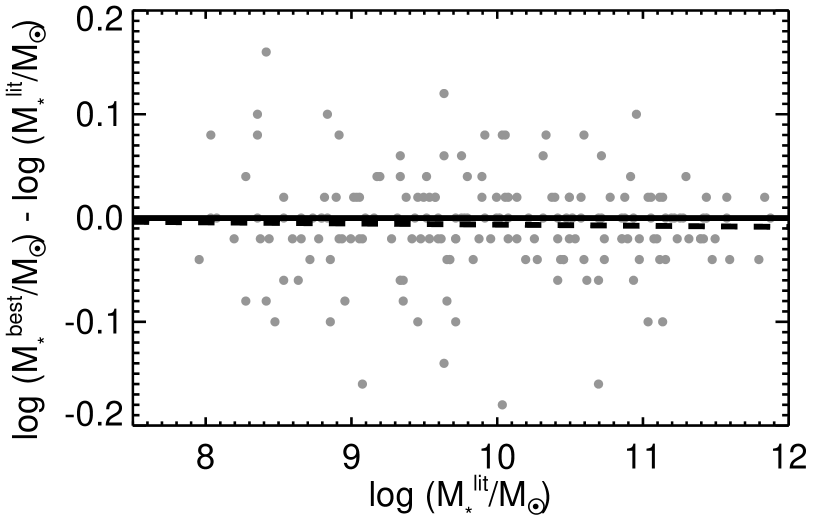
Figure 1.— Difference between the highest quality stellar masses for the NFGS (log M${}_{*}^{\rm best}$, calculated from $UBR$, SDSS, 2MASS, and IRAC photometry plus integrated spectroscopy) and stellar masses for the same galaxies estimated with data available for our literature sample (Log M${}_{*}^{\rm lit}$, calculated using only our custom SDSS and 2MASS photometry), testing the quality of stellar masses for our literature sample. The solid horizontal line represents 1:1 agreement, while the dashed line shows the ordinary least-squares fit with outlier rejection, which is not different at a statistically significant level. The scatter has negligible effect on our results.

2.3.3 Blue-Centeredness

To track enhancements in recent central star formation, we rely on a simple measure of the color gradient referred to as blue-centeredness ($\Delta C$), defined as the outer disk color from the half-light radius ($r_{50}$) to the 75% light radius ($r_{75}$) minus the color from the center to $r_{50}$ (Jansen et al. 2000b). For future reference, general discussion of blue-centeredness will use the notation, $\Delta C$, while specific discussion involving a particular color will note that color explicitly, e.g. $\Delta(g-r)$. The radii in this definition reliably separate bulge/disk colors without being sensitive to variations in bulge-to-disk ratio (Kannappan et al. 2004). The half-light radius is a natural separator of inner/outer galaxy growth; for example, Peletier & Balcells (1996) note shifts in colors and ages at approximately this radius. We also stress that this simple measure appears robust to variations in the dividing radii. For example, using the 40% and 90% enclosed light radii returns approximately the same results.

Before blue-centeredness is used to measure enhancements in recent central star formation, we account for other galaxy properties that may affect the color gradients. Kannappan et al. (2004) find that blue-centeredness correlates with galaxy luminosity, likely due to the fact that both metallicity and stellar population age can influence galaxy color gradients, reddening galaxy centers with increasing luminosity. These authors remove the luminosity trend by subtracting off the fitted relation between $\Delta(B-R)$ and luminosity. We follow the same approach, performing an ordinary least-squares fit (Isobe et al. 1990) of $\Delta C$ against stellar mass (Figure 2). We derive the following relations:

$$\Delta(u-r)=\left(-0.114\pm 0.025\right)\log{M_{*}}+\left(0.983\pm 0.249\right)$$ (4)

$$\Delta(u-g)=\left(-0.064\pm 0.017\right)\log{M_{*}}+\left(0.556\pm 0.167\right)$$ (5)

$$\Delta(g-r)=\left(-0.049\pm 0.009\right)\log{M_{*}}+\left(0.417\pm 0.095\right)$$ (6)

The use of an ordinary least-squares fit of $y$ vs. $x$ is crucial, since in order to remove any trend with stellar mass, we must minimize the scatter in $\Delta C$ relative to stellar mass. Following Kannappan et al. (2004), we calibrate this mass correction using the NFGS sample (not just our subset with CO data) since it is our most representative data set and has the most robust stellar mass estimates. The fit is limited to star-forming disk galaxies, identified as galaxies with morphology S0 or later and either detected H$\alpha$ emission extending beyond the nucleus or $U-K<4$, which helps exclude quenched galaxies (Kannappan & Wei 2008, K13s). We reject galaxies with known strong AGN and restrict the fit to $M_{*}>10^{8.5}M_{\odot}$, avoiding the low M_∗ tail of the NFGS where all blue-centeredness states may not be evenly represented. In total, 135 NFGS galaxies were used to derive these relations. The residuals of this fit give mass-corrected blue-centeredness (denoted by $\Delta C^{m}$). In simple terms, $\Delta C^{m}$ is a measure of the color difference between the inner and outer regions of a galaxy, relative to the typical color difference for galaxies at a given stellar mass, where higher values imply bluer centers. More physically, this parameter tracks recent central star formation relative to the typical star-forming galaxy at a given stellar mass.

We find that galaxies with and without strong peculiarities (i.e., signs of recent interactions) as defined by Kannappan et al. (2004) have different underlying distributions of $\Delta(g-r)^{m}$ at a 99% confidence level, so our definition of mass-corrected blue-centeredness successfully recreates the correlation found by these authors using luminosity-corrected blue-centeredness (their Fig. 8). However, we stress that while our mass correction is physically motivated, it is modest, and the distributions of uncorrected $\Delta(g-r)$ for peculiar/non-peculiar galaxies differ at confidence level comparable to that for distributions using $\Delta(g-r)^{m}$. Our general results presented in § 3 are still found without the correction in place, as discussed in § 3.2.2.

Within this paper, the total error budget on $\Delta C^{m}$ includes contributions from the measurement error of $\Delta C$, as well as additional uncertainties due to the error in $r_{50}$ and $r_{75}$, the error in the stellar mass, and the uncertainty in the fitted relation between $\Delta C$ and stellar mass. In the majority of cases, the Poisson error is dominant.

Figure 2.— $\Delta(g-r)$ versus ${\rm log\,(M_{*}/M_{\odot})}$, illustrating the correlation between blue-centeredness ($\Delta C$) and stellar mass. To isolate the effect of recent central star formation enhancements, we remove the stellar mass trend using an ordinary least-squares fit, minimizing scatter in blue-centeredness relative to stellar mass

. The residuals of this fit give mass-corrected blue-centeredness ($\Delta C^{m}$), which measures outer minus inner color relative to the typical value for a galaxy at a given stellar mass, allowing us to trace recent central star formation enhancements above the norm.

We note that optical color gradients have advantages over direct star formation rate tracers (e.g., FUV+24$\mu m$) for the purposes of our study. A practical advantage is that the data needed to compute color gradients are readily available for most galaxies. In addition, the longer timescales over which optical indicators remain sensitive to enhanced star formation are more useful for studying the extended evolution of galaxies. They enable us to analyze the stellar populations beyond the timescale of the star formation and gas consumption itself, allowing us to note the longer term consequences of recent star formation episodes. We defer a detailed analysis of the timescales of these optical indicators to future work, but Figure 11 of Kannappan et al. (2004) shows a simple model wherein the blue-centeredness fades on the order of 0.5–2 Gyr after the central star formation episode ends. It should be noted that this model represents a single case, and the evolution of blue-centeredness may vary depending on the duration and size of the burst as well as the composition of the preexisting stellar populations in the bulge and disk.

For consistency and since the vast majority of our galaxies have SDSS data, we always quote $\Delta C^{m}$ using SDSS-equivalent colors. A handful of galaxies from our NFGS sample do not have SDSS data, but do have $UBR$ photometry. We derive the following conversions between the NFGS $UBR$ and $ugriz$ systems using colors measured within the $B$ band 25 ${\rm mag\,arcsec^{-2}}$ isophote for 183 NFGS galaxies:

$$g-r=0.62(B-R)-0.18;\sigma=0.04$$ (7)

$$u-g=1.16(U-B)+1.08;\sigma=0.16$$ (8)

$$u-r=0.91(U-R)+0.61;\sigma=0.21$$ (9)

These relations are useful only for the NFGS due to the possibly different $UBR$ zeropoints used in the NFGS relative to other photometric studies (see K13s). The relations have been corrected for foreground extinction, although as we are measuring color differences, both foreground extinction corrections and k-corrections cancel. Where these conversions are used, their uncertainties are incorporated into the final error on $\Delta C^{m}$.

2.3.4 Internal Extinction Effects

Since we make use of optical color gradients, internal dust extinction is a concern. A systematic effect from dust may manifest itself as a dependence on inclination, since higher inclination galaxies show more dust along the line of sight. To determine whether internal extinction is systematically biasing our results, we run Spearman rank tests on all star-forming disk galaxies in the NFGS with measured inclinations $>$15^∘ after excluding AGN. We find no significant correlation between inclination and $\Delta C^{m}$. Shown in Figure 3, the same rank test for galaxies with stellar masses above $\sim 10^{9.7}\,M_{\odot}$ – roughly equivalent to the 120 km s^-1 rotation velocity threshold above which dust lanes become more prominent in galaxies (Dalcanton et al. 2004; see also K13s) – implies somewhat significant correlations (3%, 5%, and 4% chance of being random for $\Delta(u-r)^{m}$, $\Delta(u-g)^{m}$, and $\Delta(g-r)^{m}$ respectively). Though weak correlations may exist, these trends are much smaller than the scatter (Fig. 3). Thus we conclude that systematic internal extinction effects should have a minimal effect on our results.

We should note that while we find only small systematic effects due to inclination, dust within galaxies will inevitably alter our color gradients if it is present. There are galaxies in our sample for which visual inspection has revealed significant dust features. These galaxies and their impact on our results are discussed in § 3 and § 4.

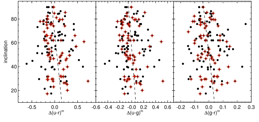
Figure 3.— Inclination versus $\Delta C^{m}$ for star-forming disk galaxies with i$>$15^∘ from the NFGS. The full sample shows no correlation between these two variables, implying no systematic effect of inclination (and associated dust extinction) on our results. Red crosses mark galaxies with stellar masses above $10^{9.7}\,M_{\odot}$, which show a weak correlations between inclination and $\Delta C^{m}$ (3%, 5%, and 4% chance of being random for $\Delta(u-r)$, $\Delta(u-g)$, and $\Delta(g-r)$ respectively). The dotted lines show the inverse least-squares fits (i.e., minimizing the scatter in the $x$-direction) to just the more massive galaxies. Any systematic effects due to inclination appear minor. However, irregular dust structures, not probed with this test, will inevitably alter color gradients (see § 3.1.1 and § 4.1.1).

2.3.5 Gas Masses

To ensure that our data are as uniform as possible, we recalculate all gas masses using the same formulae. The HI mass is calculated as (Haynes & Giovanelli 1984):

$$M_{\rm HI}=2.36\times 10^{5}D^{2}F_{21}$$ (10)

Here, $F_{21}$ is the measured 21cm flux in Jy km s^-1 and $D$ is the distance to the galaxy in Mpc. The molecular gas mass is estimated as (Sanders et al. 1991):

$$M_{\rm H_{2}}=1.18\times 10^{4}\left(\frac{X_{\rm CO}}{3\times 10^{20}}\right)D^{2}F_{\rm CO}$$ (11)

Here, F_CO is the measured CO flux in Jy km s^-1. We assume a constant X_CO of $2\times 10^{20}$ cm^-2 (K km s^-1)^-1 (Strong & Mattox 1996; Dame et al. 2001); see § 3.1.3 for an analysis of how assuming constant X_CO may affect our results. In further analysis, we multiply all gas masses by a factor of 1.4 to account for helium.

2.3.6 Beam Corrections

The majority of our CO flux measurements come from single dish telescopes with single pointings at galaxy centers. Unlike 21cm beams, which are typically several times the size of our galaxies, the CO beams are often comparable to or smaller than our galaxies. However, since CO scale lengths are typically smaller than optical scale lengths, this size mismatch is not always a major issue when trying to estimate total H₂ mass. By modeling the beam pattern of the telescope and assuming a CO flux distribution, one can estimate the additional flux not detected by a single pointing. We apply beam corrections to our single-dish CO data following the same method as Lisenfeld et al. (2011). The aperture correction is defined as the ratio of the total-to-observed CO intensity,

$$f=I_{\rm CO,total}/I_{\rm CO,observed}$$ (12)

We assume that the CO distribution $I_{\rm CO}$ follows an exponential disk,

$$I_{\rm CO}(r)=I_{0}e^{-r/h_{\rm CO}}$$ (13)

where $h_{\rm CO}$ is the scale length of the CO emission. The total CO intensity is simply the integral of this CO distribution to infinity:

$$I_{\rm CO,total}=\int_{0}^{\infty}{2\pi I_{0}re^{-r/h_{\rm CO}}dr}=2\pi I_{0}h_{\rm CO}^{2}$$ (14)

The observed CO intensity is the integral of the CO distribution convolved with the beam pattern. Assuming a Gaussian beam with HPBW, $\Theta$, this is written:

$$I_{\rm CO,observed}=4I_{\rm CO}\int^{\infty}_{0}{\int_{0}^{\infty}{\exp{\left(-\frac{\sqrt{x^{2}+y^{2}}}{h_{\rm CO}}\right)}}}$$

$$\times\exp\left(-\ln{2}\left[\left(\frac{2x}{\Theta}\right)^{2}+\left(\frac{2y\cos{i}}{\Theta}\right)^{2}\right]\right)dxdy$$

A major uncertainty in this calculation is the value of $h_{\rm CO}$. Studies of star-forming late-type galaxies have shown $h_{\rm CO}\sim(0.2\pm 0.05)R_{\rm 25}$, where $R_{\rm 25}$ is the $B$-band 25 ${\rm mag\,arcsec^{-2}}$ isophotal radius (Young et al. 1995; Leroy et al. 2008; Schruba et al. 2011). We assume this relation holds for all late type galaxies in our sample. Whether the same is true for E/S0 galaxies is uncertain, as their CO scale lengths have not been as thoroughly studied in the literature. We examine the CO profiles of Wei (2010; see also Wei et al. 2010b), who mapped the CO(1-0) distribution in a sample of E/S0 galaxies using the CARMA array. We find an average value of $h_{\rm CO}=0.1R_{\rm 25}$ with a standard deviation of 0.05$R_{\rm 25}$. We adopt this scale length for all E/S0 galaxies in our sample. It should be noted that these radial profiles are primarily for blue-sequence E/S0s, not the more common red-sequence E/S0s, simply because CO is more often detected in the former. The two red-sequence E/S0 galaxies in the Wei (2010) sample have CO scale lengths close to 0.05$R_{\rm 25}$, but two data points are not enough to warrant separate definitions of $h_{\rm CO}$ for red- and blue-sequence E/S0s.

We assume uncertainties in h_CO of 0.05$R_{25}$ for both spiral and E/S0 galaxies. The additional uncertainty that propagates into the beam-corrected H₂ mass depends on the size of the galaxy relative to the beam. Within our final sample (see § 2.3.7) additional uncertainties are on the order of 5%, though some are as large as 25%. We also note that for galaxies in our sample for which we have both single dish CO fluxes and resolved CO maps from Wei (2010), we adopt the CO fluxes from the single dish observations and beam-correct these fluxes using the measured scale-lengths from the CO maps.

2.3.7 Useability Criteria

After identifying from our NFGS+literature compilation all galaxies with the necessary optical/NIR imaging as well as 21cm and CO(1-0) flux measurements (627 galaxies), we institute a number of usability criteria that galaxies must pass before they are included in our final sample. These are: (1) SDSS $r$-band half-light radii larger than 5” to ensure blue-centeredness calculations are not compromised by variations in the PSF between the different SDSS passbands; (2) minimal beam corrections to detected CO fluxes, so that the corrected CO fluxes are no larger than 1.5 times the measured fluxes (equivalent to a change in ${\rm H_{2}/HI}<0.2$ dex), ensuring the estimated H₂ masses are minimally dependent on the assumed model of the CO distribution; (3) strong upper limits on total H₂ masses, i.e. where CO detections are missing but HI detections are not, H₂/HI must be $<0.05$. We do not remove any galaxies with HI upper limits from our sample. With these cuts, our NFGS+literature sample totals 323 galaxies. Included in this tally are 11 galaxies we judged to be highly peculiar/interacting whose derived position angles and ellipticities carry little meaning, and whose blue-centeredness calculations are therefore untrustworthy; we consider their properties in § 3.1.2. We also include an additional 122 “quenched” galaxies (two of which are also counted as highly peculiar), which pass all useability criteria except for having upper limits in both HI and H₂ mass; these are discussed in § 3.2.3. For our NFGS sample, upper limits from the IRAM 30m telescope are preferred over the ARO 12m telescope since they are always stronger. Weak upper limits led to the removal of 4 out of 39 NFGS galaxies with CO data from our final sample, though 3 of the 4 were upper limits from prior CARMA observations (Wei et al. 2010b). Where we have both IRAM 30m telescope and ARO 12m telescope detections for our NFGS sample, we prefer the IRAM 30m data as long as the beam correction is less than 1.5. Otherwise, we use the ARO 12m data.

It is important to note that while our sample is diverse, it is not statistically representative of the galaxy population since our combined data set is subject to whatever biases exist in past CO studies. Nonetheless, our useability criteria, which enforce minimum and maximum apparent radii for many galaxies in our sample, do not appear to bias us towards galaxies of a certain physical size thanks to the wide variety of distances within our sample. The distributions of physical sizes of our galaxies before and after we institute our useability criteria are not significantly different, as confirmed by a K-S test. Our final sample includes some galaxies taken from the NFGS, which were in fact originally chosen to be representative of the galaxy population (see § 2.1.1). We will use this subset to investigate our results in the context of a broadly representative data set.

Our final sample, including the quenched and peculiar galaxies, is shown on the $u-r$ color versus stellar mass plane in Figure 4. This sample includes some galaxies with M${}_{*}<10^{8.5}\,M_{\odot}$, although the blue-centeredness mass-correction was calibrated with only galaxies above this mass. These lower mass galaxies do not show unusual behavior within our results, and are therefore kept in our final sample (see § 3.2.2 for further discussion).

Our final compiled data set is made available in machine readable format in the online edition of our paper. A summary of the data is given in Table 3.

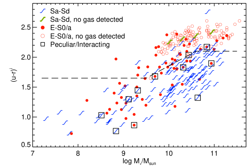
Figure 4.— Our final NFGS+literature sample plotted in $(u-r)^{i}$ versus stellar mass space. The dashed line represents the red/blue sequence divider, which is based on the analysis of Moffett et al. (2013, in prep.), which identifies the midpoint between the two sequence peaks at each stellar mass. Our red/blue sequence divider is shifted redder than this midpoint by $+$0.1 mag. The superscript $i$ indicates that an internal extinction correction has been applied following Moffett et al.

3. Results

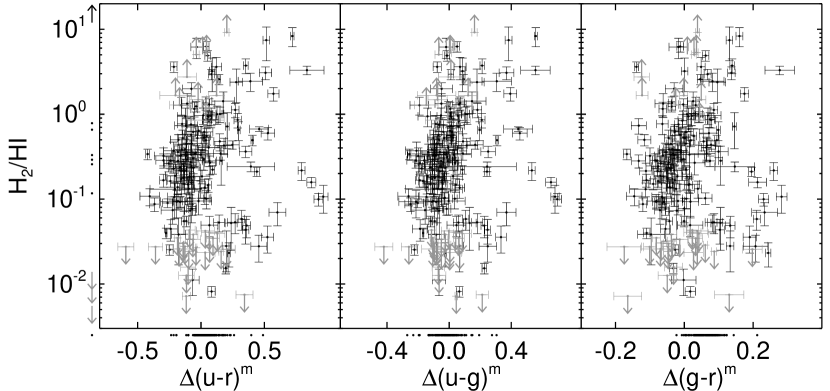
Figure 5.— Relationship between H₂/HI and mass-corrected blue-centeredness shown using three different color gradients. Grey points denote lower and upper limits in H₂/HI. To the left of the $y$-axis are dots representing H₂/HI values for galaxies with peculiar morphologies, many clearly interacting. Due to their disturbed state, we cannot measure $\Delta C^{m}$. Below each $x$-axis are dots showing the measured $\Delta C^{m}$ for quenched galaxies. All three panels show distinct loci and an empty region between them.

In this section, we describe our findings on the relationship between global H₂/HI and mass-corrected blue-centeredness. These variables are plotted in Figure 5, which we hereafter refer to as the “fueling diagram,” since it links the fraction of gas available as direct fuel for star formation and a tracer of recent interactions that drive the fueling.

In § 3.1.1, we examine the basic structure of the fueling diagram, which is broken up into three branches. The left branch holds most galaxies and shows a positive correlation between H₂/HI and $\Delta C^{m}$, consistent with the idea that molecular gas content is systematically linked to galaxy interactions as traced by mass-corrected blue-centeredness. The right and bottom branches are well-defined loci that deviate from this expected trend, showing first increasing then decreasing mass-corrected blue-centeredness as H₂/HI decreases.

In § 3.2, we explore the properties of galaxies within each branch. The left branch is largely occupied by a mix of barred and unbarred spiral galaxies, with a wide range of stellar masses and gas fractions. Conversely, the right and bottom branch are almost completely populated by low mass E/S0 galaxies, specifically blue-sequence E/S0 galaxies.

Lastly, in § 3.3 we use differences in optical color gradients to explore the evolution of galaxies within the fueling diagram. We find no preferred direction of evolution along the left branch, while the galaxies on the right/bottom branches appear to be evolving in a clockwise fashion back towards the left branch. Intriguingly, along this path there are systematic increases in total gas content and a transition from E/S0 to spiral morphology, which may signal a major transformation as these galaxies progress back towards the left branch on the fueling diagram. We collect and interpret these findings in § 4.

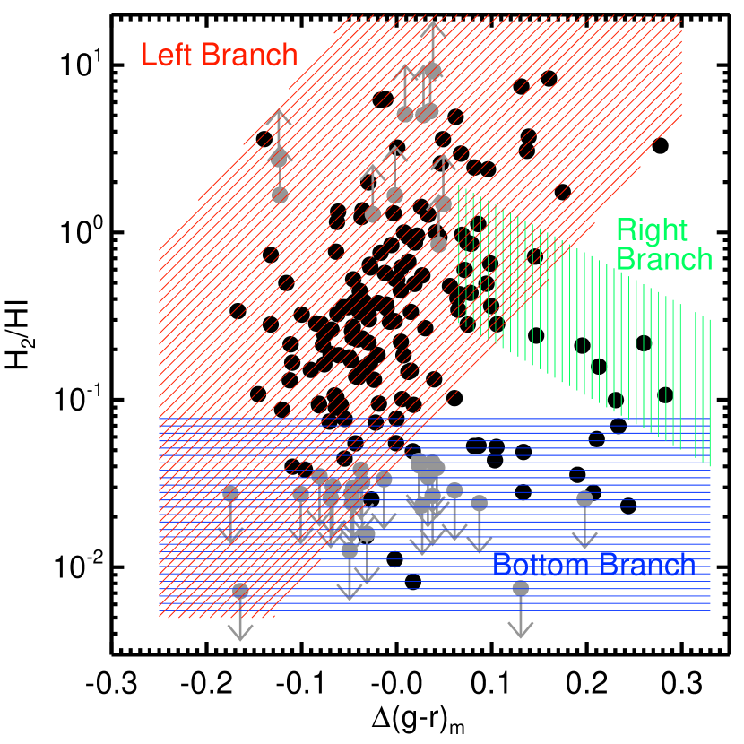
Figure 6.— Empirically defined branches in H₂/HI vs. $\Delta C^{m}$ space. These data points are the same as in Figure 5c.

3.1. The Distribution of Galaxies in the Fueling Diagram

3.1.1 The Three Branches

The fueling diagram is shown in Figure 5, plotted using mass-corrected blue-centeredness based on $u-r$, $u-g$, and $g-r$ colors, all of which recreate the same basic structure. The regions of parameter space roughly defining the left, right, and bottom branches are overlaid on the $\Delta(g-r)^{m}$ data in Figure 6.

The majority of our sample falls on the left branch, which shows a positive correlation between H₂/HI and mass-corrected blue-centeredness. There is considerable scatter which appears to increase above H₂/HI$\sim$0.5, predominantly biasing galaxies towards lower $\Delta C^{m}$. We attribute at least some of this scatter to centrally concentrated dust. Visual inspection has shown several of the galaxies that scatter to the left of the main trend have distinct dust features (e.g., M82, which lies at $\Delta(g-r)^{m}=-0.14$ and H₂/HI=3.6). Galaxies in the “dusty zone” do not have preferentially high inclination (§ 2.3.4). Rather, their centrally concentrated dust may reflect a shared evolutionary state (see § 4.1.1). The right branch of the fueling diagram, which begins to appear at $\Delta(g-r)^{m}\sim 0.05-0.1$, is far less populated but still well defined. It shows a relationship opposite to the left branch, where mass-corrected blue-centeredness increases while H₂/HI decreases. The bottom branch, which encompasses galaxies below H₂/HI$\sim$0.06, shows no clear correlation between H₂/HI and mass-corrected blue-centeredness.

Among the galaxies in our sample with gas detections and reliable $\Delta C^{m}$ measurements, $\sim$75% are on the left branch, $\sim$5% are on the right branch, and $\sim$20% are on the bottom branch. However, these percentages are very crude since the branches connect with each other and their definitions are not exact. We also stress that our sample is not statistically representative of the galaxy population, largely because of the lack of CO measurements for low-mass galaxies. Thus, the fractions of galaxies falling on the left, right, and bottom branches in Fig. 5 cannot be used to infer the true frequency with which galaxies fall on these parts of the fueling diagram. If instead we limit ourselves to the more representative NFGS subsample, the fractions of galaxies on the left, right, and bottom branches are roughly 65%, 10%, and 25%. But again, this subsample is only approximately representative.

Between these three branches exists a region where no data points lie. This hole is clearest in the version of the fueling diagram using $\Delta(g-r)^{m}$ because the right/bottom branches are most evenly populated. For this reason, we default to using the $\Delta(g-r)^{m}$ version of plot to show further results.

3.1.2 Is the hole real?

The structure seen in the fueling diagram – particularly the unoccupied region between the three branches – does not appear to be artificially created by our sample restrictions. As described in § 2.1, our full NFGS+literature sample was unrestricted in terms of stellar mass, gas content, and star formation properties. Subsequent restrictions applied were mostly related to the useability of the data. The only selection criterion we can reasonably relax is our limit on the level of permitted CO beam-correction used to estimate flux missed by the telescope beam. As discussed in § 2.3.6, we enforce the corrected-to-measured CO flux to be less than 1.5. After relaxing the corrected-to-measured CO flux to be less than 2, 5, and 10, the three branches of the fueling diagram remain well defined (although with increased scatter) and no new galaxies appear to invalidate the existence of the empty region between the branches.

It is interesting to examine whether peculiar or actively interacting galaxies could potentially fill the empty region. These galaxies lack reliable $\Delta C$ measurements, so we do not plot them within the fueling diagram. However, we mark their measured H₂/HI to the left of the $y$-axis in Figure 5. Their H₂/HI values do not exclusively cluster in the range spanned by the hole, although some have the proper values to fall within it. We conclude that if galaxies like those represented in our sample ever fall in the empty region, they must do so only briefly during a phase of rapid evolution. The specific reasons why galaxies rarely settle in this region of parameter space are not immediately apparent. Detailed modeling of galaxies may be necessary to explain this phenomenon and will be the focus of future work.

3.1.3 X_CO Effects

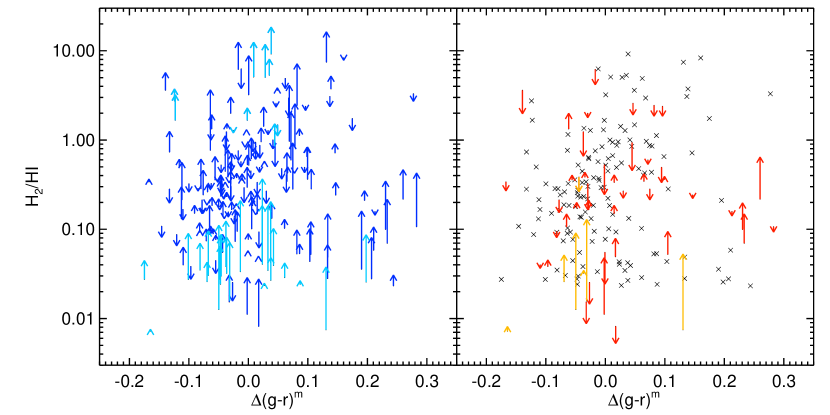
Figure 7.— The possible effect of variations in X_CO on our data, with X_CO estimated separately for each galaxy using $B$-band luminosity (left) and log(O/H) derived from nebular emission lines (right). Lighter arrows denote galaxies with H₂/HI upper or lower limits, and X’s denote galaxies where log(O/H) is unavailable. Some upper limits show significant adjustments, but X_CO variations do not change the overall appearance of three distinct branches.

The structure of galaxies in the fueling diagram appears robust against possible variations of X_CO due to its dependence on metallicity. To test this, we use O/H to estimate X_CO for each galaxy, employing the calibration from Obreschkow & Rawlings (2009). Estimates of O/H from optical line ratios are only available for our NFGS (Kewley et al. 2005) and SINGS (Moustakas et al. 2010) samples and the studies of Barone et al. (2000) and Taylor et al. (1998). To be able to carry out this analysis for our full sample, we also estimate X_CO for each galaxy from $B$ band luminosity, again using the calibration of Obreschkow & Rawlings (2009), who find it to be the next most reliable estimator of X_CO after metallicity. The values of 12+$\log{O/H}$ in our sample (where known) range from 7.9–9.2, yielding X_CO estimates between 0.4 and 10 times the Milky Way value. The calibration using $B$-band luminosity yields a similar range of X_CO.

Figure 7 shows the effect that variable X_CO due to metallicity has on the fueling diagram. Even with the variation in X_CO, the right/bottom branches remain distinct from the left branch and the hole remains intact, although some of the upper limits on the bottom branch show significant increases in H₂/HI due to their estimates of X_CO being several times the Milky Way value. These galaxies are mainly dwarfs with stellar masses $\lesssim$ a few $\times 10^{8}M_{\odot}$, where this sort of deviation might be expected. In general however, the structure of the fueling diagram remains unchanged.

The above analysis ignores other physics that may alter X_CO. Most relevant to our study is the possible decrease in X_CO in very high gas surface density regimes where the the ISM turns almost entirely molecular. Such a situation could occur as the result of inflows that drive large amounts of gas to the centers of galaxies, and has been observed in many systems from ULIRGs to ordinary spirals (Downes et al. 1993; Regan 2000). The gas in these extremely high surface density regions is expected to have increased temperature relative to molecular clouds in less dense environments (Narayanan et al. 2012), which would be coupled with an increase in the $F_{\rm CO(2-1)}/F_{\rm CO(1-0)}$ ratio. Where available, we compare $F_{\rm CO(2-1)}/F_{\rm CO(1-0)}$ (both beam corrected as in § 2.3.6) with mass-corrected blue-centeredness and H₂/HI, but we find no correlations. Any evidence of increased central gas temperature is likely being washed out in our global CO measurements. Even if some of the increase in H₂/HI with $\Delta C^{m}$ along the left branch is the result of overestimated X_CO, this is still consistent with our physical interpretation that the left branch of the fueling diagram is the result of galaxy interactions and inflows (see § 4.1.1).

For the remainder of this paper, we use molecular gas masses estimated as described in § 2.3.5, assuming constant X_CO.

3.2. Distribution of Galaxy Properties Within the Fueling Diagram

Having established the basic structure of the fueling diagram and its reliability, we now explore how galaxy properties – specifically morphology, the presence of a bar, stellar mass, blue versus red sequence, and gas content – distribute themselves throughout the fueling diagram. Doing so may provide an understanding of the physical processes that drive the observed trends. The galaxy properties discussed in this section are overlaid on the fueling diagram in Figure 8 and briefly summarized in § 3.2.6.

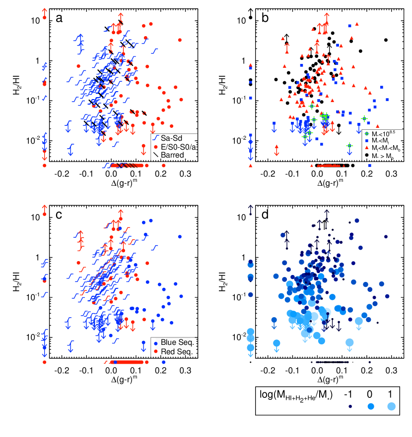
Figure 8.— (a) Distribution of early (E/S0 - S0a) and late (Sa-Sd) morphologies and bars. (b) Distribution of stellar masses in three fundamental mass regimes: stellar mass above $M_{b}$, between $M_{t}$ and $M_{b}$, and below $M_{t}$, where M_b is the bimodality mass ($10^{10.5}M_{\odot}$) and $M_{t}$ is the gas-richness threshold mass ($10^{9.7}M_{\odot}$). Also marked are galaxies that fall below the range of our blue-centeredness mass-correction. See § 3.2.2 for more details on these mass regimes. Galaxies with stellar masses outside the mass regime used to calibrate the blue-centeredness mass correction are also noted (c) Distribution of red and blue sequence galaxies (d) Distribution of $M_{\rm HI+H_{2}+He}/M_{*}$.

3.2.1 Morphology

Figure 8a displays galaxy morphologies within the fueling diagram. All galaxies are classified by eye using SDSS $g$-band images, but we check our classifications against previously published types when available. Galaxies are separated into two categories: E/S0s (including S0a) and spirals (Sa–Sd). Using the distinction between S0a and Sa as the separation between early- and late-type galaxies may be somewhat sensitive to classification error, but this division is useful since the presence or absence of extended spiral arms represents a basic transition in structure likely strongly linked to star formation history.

We find a clear bimodality in the distribution of E/S0 and spiral morphologies. Spiral galaxies almost exclusively fall on the left branch, and in fact, a Spearman rank test on all spiral galaxies with H₂/HI$>$0.06 (to avoid confusion with the bottom branch) confirms a correlation between H₂/HI and $\Delta C^{m}$, with $\sim$5$\sigma$ confidence (for $u-r$, $u-g$, and $g-r$, the probabilities of the distributions being random are $5\times 10^{-8}$, $8\times 10^{-7}$, and $1\times 10^{-7}$ respectively). E/S0s show a much more diverse distribution throughout the fueling diagram: some occupy the left branch with spirals, but also and more noticeably the rest almost completely define the right branch and much of the bottom branch. Several of the E/S0s on the right/bottom branches are also centrally concentrated Blue Compact Dwarf galaxies (BCDs), which are lumped with traditional E/S0s in our simplified morphological classification scheme. Towards the left end of the bottom branch, there is a strong shift in morphology from E/S0 to spiral.

Barred galaxies are also shown in Figure 8a. Except for galaxies that have existing bar classifications from the NFGS or Nair & Abraham (2010), bar classifications were done by eye using SDSS $i$-band imaging, since bars are best identified in bands that trace the stellar light (Eskridge et al. 2000). Bars are noticeably absent from all galaxies above $\Delta(g-r)^{m}\sim 0.15$, which includes most of the right branch, as well as sections of the left and bottom branches. Within the left branch alone, a Spearman Rank test does not suggest a smooth correlation of bar fraction with $\Delta C^{m}$ or with H₂/HI. Although our full sample is not statistically representative of the galaxy population, we speculate that the same processes that produce extreme blue-centeredness may destroy bars, while milder processes associated with evolution along the left branch do not. If we limit our examination of bars to only the more representative NFGS subsample, we still see no significant trend between $\Delta C^{m}$ and bar fraction within the left branch. Bars are important galactic structures to put into the context of our study, since like galaxy interactions, they are thought to enable inflows of gas to the centers of galaxies. We discuss bars and interpret their role in § 4.3.

3.2.2 Stellar Mass

Figure 8b displays the distribution of stellar masses within the fueling diagram. Instead of examining the continuous distribution of stellar masses, we divide the data into three characteristic mass regimes: (1) $M_{*}>M_{b}=3\times 10^{10}\,M_{\odot}$, where $M_{b}$ is the bimodality mass, a stellar mass scale above which the population of galaxies goes from being typically star-forming with disk-like morphology to typically non-star-forming with spheroidal morphology (Kauffmann et al. 2003), (2) $M_{*}<M_{t}=5\times 10^{9}\,M_{\odot}$, where $M_{t}$ is the gas-richness threshold mass, below which there is a significant increase in gas-dominated galaxies (Kannappan et al. 2009, K13s), and (3) $M_{t}<M_{*}<M_{b}$, where bulged spirals with intermediate mass content are the norm (K13s). Galaxies with $M_{*}<10^{8.5}\,M_{\odot}$ are also denoted with an extra “$+$” symbol in this figure. These galaxies technically fall outside the stellar mass range used to calibrate the blue-centeredness mass-correction (§ 2.3.3), and Kannappan et al. (2004) suggest their possibly irregular patterns of star-formation may make color gradients hard to interpret in relation to higher mass galaxies. However, we include them in our plots because they show no unusual distribution relative to the rest of the sample below M_t. Among these galaxies, the most extreme blue-centeredness is found for NGC 3738, with $\Delta(g-r)^{m}=0.19$. This galaxy is a centrally concentrated BCD, making it completely consistent with its neighboring galaxies in the fueling diagram.

The different stellar mass regimes display patterns within the fueling diagram. While galaxies in all three regimes span the full range of H₂/HI, we find almost no galaxies above $M_{b}$ on the right/bottom branches. Instead, most of the galaxies on these branches fall below $M_{t}$. There is also a tendency for galaxies below $M_{t}$ to cluster in the lower-left corner of the fueling diagram (many having H₂/HI upper limits), but elsewhere along the rising branch they appear to spread roughly evenly, as do galaxies in the higher stellar mass regimes. We note that with our low number statistics, the apparent tendency of galaxies on the upper right branch to have stellar masses between M_t and M_b is not significant and should not be over-interpreted given that the range between M_t and M_b is very narrow, and stellar mass estimation involves typical errors of $\sim$0.2 dex.

In § 2.3.3, we described our motivation and methods for subtracting the underlying dependence of blue-centeredness on stellar mass, yielding mass-corrected blue-centeredness, or $\Delta C^{m}$. To determine how dependent our results are on this mass correction, we plot the fueling diagram using the uncorrected $\Delta(g-r)$, rather than $\Delta(g-r)^{m}$, in Figure 9. The general structure of the fueling diagram remains intact, specifically the presence of three branches with a hole between them. The distribution of different mass regimes illustrates the tendency of high-mass galaxies to have more red-centered color gradients, which originally motivated our mass correction.

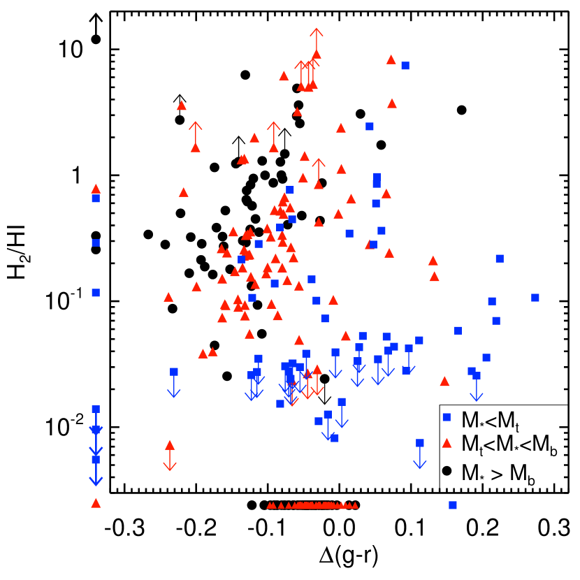
Figure 9.— The fueling diagram plotted using blue-centeredness without a mass correction. Without the mass correction applied to blue-centeredness, there is a tendency for higher stellar mass galaxies to have more red-centered color gradients (motivating the mass correction), but the underlying structure of the fueling diagram remains intact.

3.2.3 Red and Blue Sequences

Figure 8c shows the distribution of red and blue-sequence E/S0s and spirals in the fueling diagram, which are classified based on their positions within the $u-r$ versus stellar mass plane shown in Figure 4. The left branch is composed of a mix of red and blue sequence galaxies. Intriguingly, the right and bottom branches are almost completely dominated by blue sequence galaxies, despite the common assumption that E/S0 galaxies always fall on the red sequence. High-mass, red-sequence E/S0 galaxies in our sample are often quenched, i.e., have no detected CO or HI emission and total gas-to-stellar mass ratio upper limits less than 0.04M_⊙. These systems are shown below the $x$-axis in Figures 5, 8, 9, and 10.

3.2.4 Gas Content

Figure 8d shows the distribution of total gas-to-stellar mass ratio (total gas = HI+H₂ with a 1.4$\times$ mass correction for He) within the fueling diagram. Broadly speaking, HI-to-stellar mass ratios and total gas-to-stellar mass ratios on the left branch are both anti-correlated with H₂/HI. However, there is significant diversity below H₂/HI$\sim$0.5, where galaxies with both very high and very low gas fractions fall. Above H₂/HI$\sim$0.5, the gas fractions on the left branch are consistently low.

Most of the galaxies comprising the right and bottom branches have substantial gas content, between 10–100% of their stellar mass. Along the bottom branch, both HI-to-stellar and total gas-to-stellar mass ratios appear anti-correlated with mass-corrected blue-centeredness, that is, gas content is higher on the left, more red-centered side. Using a Spearman rank test on all unquenched bottom branch galaxies (defined as H₂/HI $<$ 0.06), we find the negative correlation of total gas-to-stellar mass ratio and $\Delta(g-r)^{m}$ has a 1.6% chance of being random. This probability drops to 0.2% when restricting the test to $M_{*}>10^{8.5}\,M_{\odot}$ (i.e., the mass above which the blue-centeredness mass correction was calibrated). A few red-sequence galaxies with very low gas fractions also lie on the bottom branch, which are among the minority of massive ($M_{*}>M_{t}$) E/S0s whose gas data are not upper limits.

3.2.5 AGN

While our sample lacks uniform/complete data for AGN classification, we display known AGN in Figure 10 and briefly discuss them for two reasons. First, it is important to note that AGN themselves are not the cause of strongly blue-centered color gradients, as their light contribution is typically too small to have any significant effect on mass-corrected blue-centeredness, which uses colors measured over large regions of galaxies. Second, we note that AGN are predominantly seen among the high mass galaxies in our sample (see also Fig. 8b), with 25 out of 27 AGN hosted by galaxies with M${}_{*}>{\rm M}_{t}$. Their presence, particularly among the high mass elliptical galaxies which show AGN in the quenched regime but also among galaxies with detected gas, affects our physical interpretation of the fueling diagram, and is discussed in § 4.1.1 and § 4.1.3.

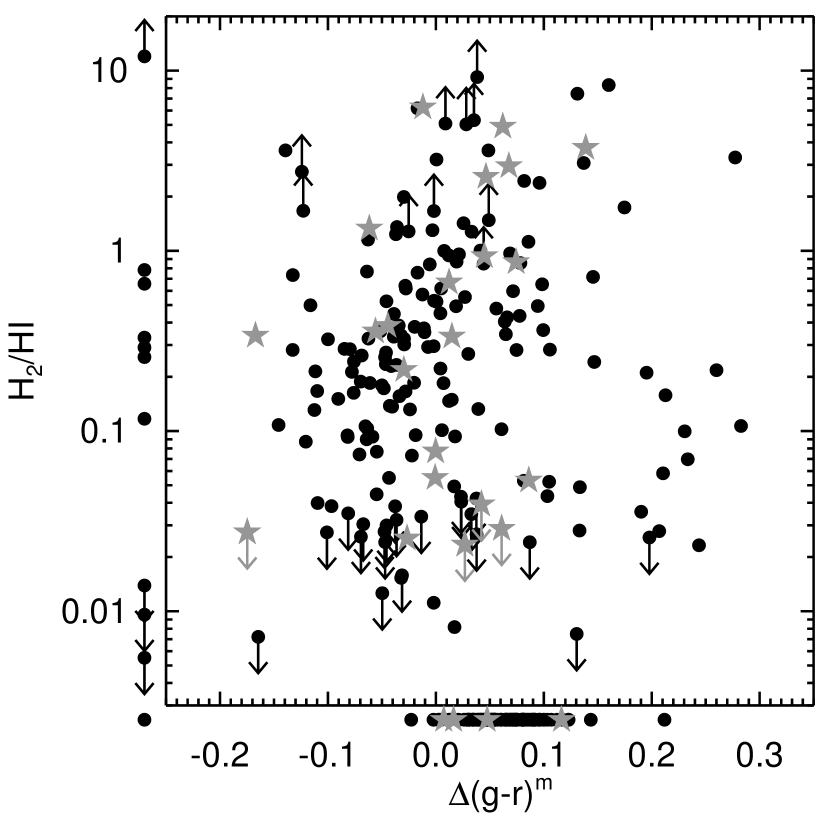
Figure 10.— Known AGN (stars) within the fueling diagram. This classification is not complete or uniform in our sample due to the limited number of classifications available in the literature and incomplete nuclear spectroscopy.

3.2.6 Properties Summary

To summarize, the main properties of each branch of the fueling diagram are as follows:

The left branch is where spiral galaxies are primarily found. Many galaxies here are barred, but without any discernible pattern with respect to $\Delta C^{m}$ or H₂/HI. Galaxies on the left branch cover the full range of stellar masses, along with a wide range of HI- and total gas-to-stellar mass ratios, which broadly behave inversely to H₂/HI.

The right and bottom branches are almost entirely populated by unbarred E/S0 galaxies, although this type distribution transitions into largely spirals on the left side of the bottom branch, which is also where we begin to see barred galaxies again. Stellar masses fall predominantly below the bimodality mass, and most fall below the threshold mass. Gas fractions are moderate to high, between 10% and 100% of the stellar mass, and show a negative correlation with mass-corrected blue-centeredness along the bottom branch.

We also note that the right/bottom branches are dominated by blue-sequence E/S0 galaxies, i.e., galaxies with spheroidal morphologies that fall on the blue sequence in color versus stellar mass space, which are thought to represent a transitional phase (Kannappan et al. 2009). This fact, as well as the properties of galaxies within the different branches of the fueling diagram, may reveal important clues as to how these branches relate to different evolutionary states, as discussed in § 4.

3.3. Do Galaxies Evolve Within the Fueling Diagram?

If mass-corrected blue-centeredness and H₂/HI are time-varying properties, galaxies should evolve within the fueling diagram. To determine whether there is any unified direction of evolution within the fueling diagram or any one of its branches, we search for systematic offsets between $\Delta(u-g)^{m}$ and $\Delta(g-r)^{m}$. This comparison is useful because $u-g$ color reddens faster than $g-r$ color after a star forming event, and therefore $\Delta(u-g)^{m}$ tracks recently enhanced central star formation over shorter time scales and will return to low values faster than $\Delta(g-r)^{m}$. Before comparing these two measurements, we must first account for the fact that the range of values for $\Delta(u-g)^{m}$ is larger than for $\Delta(g-r)^{m}$ (see Figure 5). We therefore divide $\Delta(u-g)^{m}$ and $\Delta(g-r)^{m}$ by their median absolute deviations (0.102 and 0.054 respectively, found with the same NFGS subsample used to derive Eqs. 4–6) to obtain normalized mass-corrected blue-centeredness values, $\Delta(u-g)^{m*}$ and $\Delta(g-r)^{m*}$, for which the values cover a similar range while not changing the position of zero (i.e., the average gradient for the population).

In Figure 11, arrows display the relative positions of $\Delta(u-g)^{m*}$ (head of arrow) and $\Delta(g-r)^{m*}$ (tail of arrow). Galaxies on the left branch are directed randomly left or right along it. This result suggests that galaxies either do not evolve throughout this region of the fueling diagram, or the evolution is not necessarily in a unified direction. Given the prior association of mass-corrected blue-centeredness with interactions (Kannappan et al. 2004; Gonzalez-Perez et al. 2011), we suppose that galaxies may oscillate along the left branch, rising when inflows enhance central star formation and H₂/HI (with some of the apparent rise in H₂/HI possibly associated with a decrease in X_CO due to the central gas concentration), and fall along the same locus as outer disk gas and star formation are renewed.

Conversely, the loop composed of the right and bottom branches shows some partial systematic behavior. Although the arrows on the right branch show no preferred direction, the bottom branch shows an excess of galaxies with $\Delta(u-g)^{m*}$ lower than $\Delta(g-r)^{m*}$, implying that these galaxies are evolving leftwards towards lower mass-corrected blue-centeredness. Ignoring the bottom-left region of the fueling diagram where the left and bottom branches cannot be distinguished ($\Delta(g-r)^{m}<0.05$), we find the frequency of leftward facing arrows on the bottom branch is higher than the frequency found on the left branch at the 4.2$\sigma$ confidence level, assuming the uncertainty in the number of rightward/leftward facing arrows follows Poisson statistics. The right and bottom branches are likely closely linked (discussed further in § 4), leading to our physical interpretation that galaxies on the right branch are still undergoing a central starburst, after which they move to the bottom branch where their young central stellar population ages and fades. If star formation is still progressing progressing on the right branch, then there may be no reliably predictable difference between $\Delta(u-g)^{m*}$ and $\Delta(g-r)^{m*}$, which would explain the lack of a unified direction of arrows for right branch galaxies in Figure 11. At this point, we do not have an estimate of the timescales associated with the evolution along the the right or bottom branches, but estimating these timescales by comparing the galaxy colors to stellar population synthesis models will be a focus of future work. We also note that the results of Figure 11 are not dependent on the stellar mass correction applied to blue-centeredness as the same result is found even without any mass correction whatsoever.

Since comparing $\Delta(g-r)^{m*}$ and $\Delta(u-g)^{m*}$ gives a clear direction of evolution along the bottom branch, we can tell that galaxies here shift from primarily E/S0 to primarily spiral morphologies, as well as generally toward increasing gas-to-stellar mass ratios. We interpret this pattern as a sign of disk rebuilding in § 4.2.

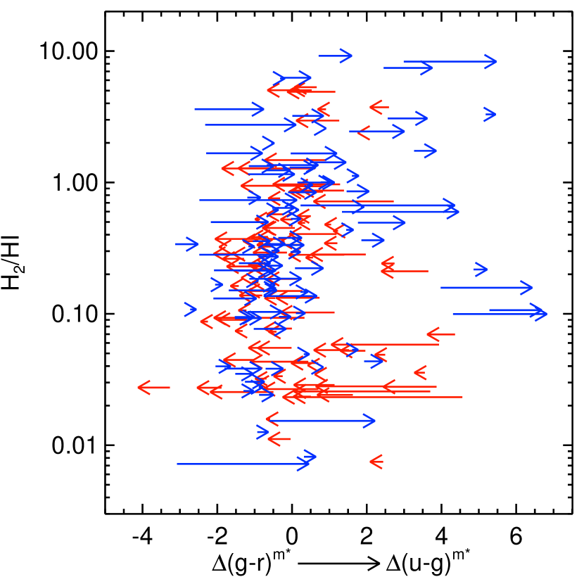
Figure 11.— Arrows going from $\Delta(g-r)^{m*}$ to $\Delta(u-g)^{m*}$. Since $u-g$ color is more sensitive to high mass short lived stars, central enhancements in $u-g$ color should be shorter lived than central enhancements in $g-r$ color. The data at the bottom branch support this expectation by showing $\Delta(g-r)^{m*}$ more blue-centered than $\Delta(u-g)^{m*}$ in most cases, indicating that these galaxies’ central star formation has ceased and the young population is fading. This color comparison suggests a uniform evolutionary direction of galaxies within this region of parameter space.

4. Discussion

In § 3 we presented the fueling diagram relating global H₂/HI to recent central star formation enhancements. Having described the three-branch distribution of galaxies within the fueling diagram, the variation of galaxy properties along and between the branches, and the apparent evolution within the diagram, we now collect these results to provide an interpretation of the physical processes that drive it. We first discuss the role of galaxy interactions in driving H₂/HI ratios, considering the importance of the merger mass ratio, stellar mass, and gas richness of the galaxies involved. We then explore how trends within the fueling diagram support a scenario of fresh gas accretion and stellar disk rebuilding along the bottom branch. We finish by reassessing the validity of the assumed link between mass-corrected blue-centeredness and galaxy interactions in light of our new results, specifically addressing the role of bars.

4.1. Mergers and Interactions in the Fueling Diagram

In the following section, we describe the role that mergers play in driving the evolution in each branch of the fueling diagram.

4.1.1 The Left Branch and Regions Above It

The very existence of the left branch provides support for the idea that local galaxy interactions play a key role in replenishment of molecular gas: since mass-corrected blue-centeredness is a signpost of recent galaxy interactions (Kannappan et al. 2004), and it is correlated with H₂/HI, galaxy interactions appear to be linked to H₂/HI in a systematic way. The analysis of $\Delta(u-g)^{m*}$ and $\Delta(g-r)^{m*}$ in § 3.3 implies that galaxies on the left branch may evolve along it in both directions: up as a result of each galaxy encounter, boosting the galaxy to higher H₂/HI and $\Delta C^{m}$ (with a possible contribution due to overluminous CO), then down as the molecular reservoir is consumed and the young central stellar population fades. Total gas-to-stellar mass ratios support this scenario. We expect HI and total gas-to-stellar mass ratios to decrease at higher $\Delta C^{m}$ since the gas is being converted into H₂ and then stars, but we also expect a mix of gas fractions at low $\Delta C^{m}$ since galaxies settle here before or after each burst event while accreting fresh disk gas. The bulk of the evolution along the left branch must be driven by minor rather than major mergers or interactions, since most galaxies appear to retain their spiral morphologies. An alternate possibility is that the relation along the left branch reflects bar-driven inflows. However, bars do not show any statistically significant correlation with $\Delta C^{m}$ along the left branch. The possible role of bars is explored further in § 4.3

Major mergers in the high stellar mass and/or low gas fraction regime may help to explain the E/S0s at high H₂/HI on the left branch (in contrast, gas-rich, low mass, but comparable mass ratio mergers appear to follow a different path; see § 4.1.2–4.1.3). Alternatively, these galaxies could be formed by repeated minor mergers rather than a single event (Bournaud et al. 2007), and they could therefore be galaxies that have made several oscillations along the left branch. Either way, many of the E/S0s at high H₂/HI on the left branch are likely moving into the quenched regime, up and off the plot, as their remaining gas reservoirs have become almost entirely molecular and may soon be completely depleted. In addition, some of the high stellar mass E/S0s at the peak of the rising branch may have previously been quenched but recently experienced small gas accretion events, possibly associated with satellite accretion (e.g., Martini et al. 2013). Some of these E/S0s host AGN, as do many of the high mass E/S0s in the quenched regime. A gas accretion event could provide fuel for AGN activity coupled with a central molecular gas concentration, resulting in a high H₂/HI ratio with minimal change to $\Delta C^{m}$ (since most of the star formation would be occurring very close to the AGN). Galaxies undergoing this process would jump vertically in the fueling diagram, between the quenched regime and the peak of the left branch. This path could place them in the hole of the fueling diagram, although they would likely move through it relatively quickly.

As previously noted in § 3.1.1, there is substantial scatter above the left branch towards more red-centered color gradients, likely caused by internal extinction. While dust effects may be altering the measured color gradients, they usefully highlight galaxies in early stages of star-forming events when the young stars are still heavily embedded in dust clouds. We suspect galaxies in this “dusty zone” represent a stage very soon after mergers or interactions that are mild enough not to have driven the galaxy into the peculiar morphology region off the plot, shown on the left hand side of the fueling diagram. As the star formation progresses, the dust is likely to clear, allowing these galaxies to develop the bluer-centered color gradients expected for their H₂/HI ratios.

4.1.2 The Right Branch

We suggest galaxies on the right branch may be the result of gas-rich mergers, specifically between galaxies of comparable stellar mass. Along with their high values of mass-corrected blue-centeredness (suggestive of a strong central starburst), the spheroidal morphologies of galaxies on the right branch are consistent with recently violent histories. Most of these galaxies are classified as blue-sequence E/S0s, and several are also classified as BCDs (e.g., Haro 2, NGC 7077, UM 465). The existence of blue sequence E/S0s and BCDs in the same regime of the fueling diagram argues in favor of them experiencing similar evolutionary processes. Previous observational and theoretical studies of BCDs (e.g., Östlin et al. 2001; Pustilnik et al. 2001; Bekki 2008) also support merger driven evolution.

While most of these galaxies do not show obvious outward signs of a recent strong interaction in their optical images, such as irregular structure or tidal features (the lack of these features is actually built in to our analysis since we do not plot highly peculiar/interacting systems), smooth optical morphology is not inconsistent with a merger having recently occurred. Merger simulations find the strongest morphological disturbances before the peak of induced star formation, which in turn typically occurs before galaxies land on the right branch, and the complete coalescence of the two merging galaxy nuclei commonly happens several hundred Myr before the main starburst event (Lotz et al. 2008, 2010). The diverse arrow directions in Figure 11 on the right branch suggest these galaxies are still actively forming stars well after the merger remnant has settled. Signatures of recent mergers may be more obvious in observations of gas morphology and kinematics. HI maps can be extremely useful since they trace extended structure and can retain signatures of interactions as long as 1 Gyr after the events (Holwerda et al. 2011). For example, the high resolution HI map of Haro 2 (Bravo-Alfaro et al. 2004) shows the HI kinematic and optical major axes to be almost perpendicular, consistent with a merger or recent accretion event.

Blue-sequence E/S0s are known to emerge primarily below M_b, and become abundant below M_t (Kannappan et al. 2009). As seen in Fig. 8, the blue E/S0s on the right branch are consistent with this pattern. However, the existence of the right branch cannot be driven by stellar mass alone. Low stellar mass galaxies are found throughout the fueling diagram, and if $\Delta C^{m}$ were dictated solely by stellar mass (i.e., equal size bursts occurring in higher/low mass galaxies yielding lower/higher $\Delta C^{m}$), then the hole seen in the fueling diagram should not exist. A merger origin for the right branch is more consistent with such a large gap between the left and right branches. Furthermore, gas richness likely produces distinct evolutionary tracks for galaxies: gas-rich mergers drive galaxies along the right branch, while gas-poor mergers drive galaxies into the quenched regime, up and off the plot, as discussed in § 4.1.1. The association of the gas-rich merger track with galaxies below M_b and especially M_t is a simple consequence of increasing gas richness below those scales (Kannappan et al. 2009, K13s).

4.1.3 The Bottom Branch

The bottom branch appears to be part of the same evolutionary sequence as the right branch but at a later stage. Galaxies here show many of the same properties as those on the right branch in terms of stellar mass, gas richness, and prominence of blue-sequence E/S0s. However, they show depressed H₂/HI ratios while uniformly evolving leftwards in the fueling diagram (§ 3.3). These observations are all consistent with a scenario where these are post-starburst galaxies with depleted central gas and fading young central stellar populations.

4.2. Evidence for Disk Rebuilding

We have argued that relatively low mass, gas-rich, but roughly equal-mass-ratio mergers appear to be responsible for the creation of blue-sequence E/S0 galaxies on the right and bottom branches of the fueling diagram. Combining the known direction of evolution on the bottom branch (§ 3.3) with the observed trends in gas-to-stellar mass ratio and morphology (§ 3.2.1,3.2.4) further implies that these galaxies may regrow gas and later stellar disks. For galaxies on the bottom branch, there is a general increase in the total gas-to-stellar mass ratio as $\Delta C^{m}$ decreases. Since galaxies here appear to be evolving leftward on the fueling diagram, their total gas content must be growing as their central stellar populations fade. In the same direction, there is a transition from E/S0 morphologies to spiral morphologies. These combined trends are consistent with a scenario of fresh outer-disk gas accretion and eventual conversion into visible spiral arms, and in fact blue-sequence E/S0s have ideal stellar surface mass densities for turning gas efficiently into stars, promoting stellar disk rebuilding (Kannappan et al. 2009; see also Kauffmann et al. 2006). Notwithstanding this self consistent picture of morphological transformation, there remain a handful of blue sequence E/S0s in the bottom left corner. One possible explanation for their presence is that spiral structure formation has been inhibited. Two examples where such inhibition may be occurring are described in Kannappan et al. (2009): NGC 7360 ($\Delta(g-r)^{m}$=0.027, H₂/HI$<$0.023), which hosts counter-rotating stellar disks, and UGC 9562 ($\Delta(g-r)^{m}$=-0.002, H₂/HI=0.011), which is a polar ring galaxy. In both of these cases, peculiar kinematics may be stifling spiral arm formation.

Falling below the gas-richness threshold mass M_t (§ 3.2.2, K13s) may enable galaxies to evolve leftward along the bottom branch. Bottom branch galaxies typically fall below M_t and have not only high gas fractions (as is typical for blue-sequence E/S0s in general, Kannappan et al. 2009, Wei et al. 2010a), but gas fractions that increase as their central starbursts fade. The high/increasing gas fractions may indicate rapid gas accretion below M_t as argued by K13s. Theoretical studies of gas accretion from the last decade might suggest that M_t reflects the critical mass scale for cold-mode accretion (Birnboim & Dekel 2003; Kereš et al. 2005). However, Nelson et al. (2013) calls this interpretation into question, arguing that there is no strong transition from cold to hot mode accretion, and that the amount of gas accreted via the cold mode is not as large as previously thought. Regardless of the mode of accretion, the high/increasing gas fractions on the bottom branch may be explained using the halo mass dependence of gas cooling times (Lu et al. 2011).

Conversely, galaxies on the bottom branch that have abnormally low gas fractions relative to the rest of the population have masses above M_t. One possible reason may be reduced accretion. Above the bimodality mass M_b in particular, both observations and theory suggest significantly quenched cosmic accretion onto galaxies (e.g., Gabor & Davé 2012, K13s). Another possible reason certain galaxies might fail to accrete fresh gas on the bottom branch is their environments. Galaxies in dense clusters and groups have long been observed to have depressed HI fractions (Giovanelli & Haynes 1985; Solanes et al. 2001; Cortese et al. 2011), and galaxies near massive companions are also more likely to be quenched, even in the dwarf regime below M_t (Geha et al. 2012). One likely example of neighbor-inhibited accretion within our sample is NGC 3073, a blue-sequence E/S0 below M_t that has an abnormally low gas-to-stellar mass ratio, but lies very close to its much larger companion, NGC 3079. The fact that NGC 3079 has an AGN and observed outflows (Cecil et al. 2001) may also be related to the low gas fraction in NGC 3073. Other outliers on the bottom branch, NGC 4111 and NGC 4270, reside in dense groups. A full environmental analysis has not been performed on our sample, but these anecdotal cases hint that environment, as well as stellar mass, likely determines which galaxies are capable of regrowing disks.

A final possible explanation of some outliers on the bottom branch may be that they never even proceeded along the right and bottom branches to reach their current locations. As discussed in § 4.1.1, these may be galaxies from the quenched regime that have experienced small accretion events, causing them to travel vertically within the fueling diagram (i.e., through the bottom branch rather than along it) as they develop/deplete small central molecular gas concentrations. In this scenario, such galaxies would only fall on the bottom branch as an accident of timing.

4.3. Revisiting the Link Between Mass-Corrected Blue-Centeredness and Galaxy Interactions vs. Bars

Throughout this paper, we have made the assumption that mass-corrected blue-centeredness is linked to galaxy interactions. This assumption is motivated by Kannappan et al. (2004), who link blue-centered galaxies to morphological peculiarities indicative of galaxy interactions. One possible issue with this assumption is that E/S0s often lack morphological peculiarities (partially by their definition of having smooth light distributions), but may still have blue centers. Therefore, it is not necessarily obvious that E/S0s have blue centers for the same reason that clearly disturbed galaxies do.

Our results argue strongly in support of the assumption that high mass-corrected blue-centeredness implies a recent galaxy encounter, even in cases where morphological peculiarities are not obvious. In fact, the galaxies that have experienced the strongest encounters without quenching (gas-rich major mergers of low-mass galaxies) are probably the blue-sequence E/S0s on the right and bottom branches that show relatively smooth structure in their optical images. A notable exception to the link between blue-centered color gradients and recent interactions is the existence of the galaxies in the “dusty” zone above the left branch, which appear to be in early, more dust-embedded stages of star formation. This implies that there is a window shortly after the start of induced star formation where mass-corrected blue-centeredness is a poor indicator of a recent interaction.

Bars have been suggested as an alternate mechanism for funneling gas to the centers of galaxies based on direct observations of gas kinematics (Regan et al. 1995; Laine et al. 1999; Regan et al. 1999). The relative importance of bars versus interactions is not well known due to a lack of large, homogeneous samples capable of adequately testing both mechanisms. Recently, Ellison et al. (2011) used the abundance of bars and close pairs in a large sample from the SDSS to argue that bars induce $\sim$3.5 times more central star formation than galaxy interactions, although the authors note that minor interactions (i.e., pairs with mass ratios larger than 3/1) are not considered in their analysis. Whether bars are a mechanism for inward gas transport completely independent of galaxy interactions is also unclear. Galaxy interactions can induce bar formation (Gerin et al. 1990; Miwa & Noguchi 1998), but at the same time bars can form in stable disks (Ostriker & Peebles 1973; Sellwood 1981), and interactions may actually destroy barred galaxies in some cases (Berentzen et al. 2003; Casteels et al. 2012). Studies of bar fractions likewise give mixed results as to whether bars are related to galaxy interactions or not (Aguerri et al. 2009; Li et al. 2009; Barway et al. 2011; Lee et al. 2012).

Bars do not appear to play any role in evolution along the right and bottom branches of the fueling diagram. In fact, they are absent in these branches, except for the region very near the junction between the left and bottom branches, which we have already argued is a spiral rebirth stage long after the inflow event that triggered the starburst. This lack of bars in the blue E/S0 population is consistent with observations of the bar frequency as a function of morphology (Nair & Abraham 2010; Barway et al. 2011; Lee et al. 2012). One could argue that bars did induce the original gas inflow and their absence on the right and bottom branches is caused by the build-up of central mass concentrations which dissipate bar structures (Norman et al. 1996; Shen & Sellwood 2004; Athanassoula et al. 2005; Bournaud et al. 2005). However, this picture would not explain why all the galaxies are E/S0s. More likely, any existing bars were destroyed by violent mergers whose remnants populate the right and bottom branches of the fueling diagram.

Bars are found on the left branch, but the bar fraction shows no smooth trend with either $\Delta C^{m}$ or with H₂/HI (although bars are absent at the top-right of the left branch), and they are even quite abundant in the bottom-left corner of the fueling diagram where galaxies show no sign of gas inflow. This lack of a smooth correlation may be explained if bar lifetimes are on the order of a few Gyr (Jogee et al. 2004; Bournaud et al. 2005; Debattista et al. 2006), in which case bars may drive gas inflow that boosts central gas concentrations and star formation but also remain well after central gas concentrations have been depleted and starbursts have ceased (Sheth et al. 2005; Wang et al. 2012, but see Ho et al. 1997 and Sakamoto et al. 1999 for alternate viewpoints). This possible longevity makes interpreting the role bars play on the left branch difficult. However, since there are galaxies near the top of the left branch without bars, they certainly do not seem to be required to initiate an inflow event. Bars may increase the strength of inflows and induce quicker depletion, but at this point it is unclear whether barred and unbarred galaxies behave systematically differently on the left branch.

5. Conclusions

Using mass-corrected color gradients and H₂/HI ratios for a sample of galaxies spanning a broad range of morphologies, stellar masses, and evolutionary states, we have analyzed the relationship between recent central star formation enhancements, likely to reflect galaxy interactions, and global H₂/HI ratios and total gas content in galaxies. We summarize our main results:

• The parameter space of global H₂/HI and recently enhanced central blueness, which we refer to as the “fueling diagram,” shows a complex relationship composed of three main branches – the left branch, the right branch, and the bottom branch – with most of our galaxies falling on the left branch. Galaxies in specific evolutionary states tend to concentrate in certain regions of the diagram (e.g., dusty, early-stage starbursts), or can be represented on one axis of the diagram (e.g., quenched systems). Since our sample is not statistically representative of the galaxy population, we cannot estimate the frequency with which galaxies fall on each branch.

• The left branch is composed primarily of star-forming spiral galaxies with a wide range of stellar masses and gas fractions. It follows a positive correlation between global H₂/HI and recently enhanced central star formation. We interpret this correlation as evidence that H₂/HI ratios are systematically linked to local encounters with other galaxies that drive inflows and replenish molecular gas reservoirs. Additionally, apparent enhancement of H₂/HI ratio measurements may be caused by decreased X_CO in the high surface density gas often found in the centers of galaxies that experience inflow events. Galaxies on the left branch likely evolve in both directions along it before and after inflow events.

• The right and bottom branches are composed almost exclusively of gas-rich blue-sequence E/S0 galaxies with stellar masses below the bimodality scale M_b and typically also below the gas-richness threshold scale M_t. Several lines of evidence suggest these two branches are part of a continuous evolutionary sequence of galaxies formed by gas-rich mergers of galaxies with roughly equal masses, which results in E/S0 galaxies that are experiencing strong central starbursts, depleting their molecular gas, and then fading back towards the left branch.

• The population of galaxies on the bottom branch evolving back towards the left branch shows a general increase in total gas content and displays a clear transition from primarily E/S0 to primarily spiral morphologies. These results strongly suggest fresh cosmic gas accretion and post-merger disk rebuilding in the low mass regime. Our current analysis does not constrain the timescale of this regrowth, but this question will be a topic of follow-up research.

• E/S0s above M_t and especially M_b do not obviously move along the branches and may instead move vertically in the plot, due to minor accretion events associated with nuclear fueling of star formation or AGN.

• Barred galaxies are common on the left branch, although the presence of a bar shows no clear correlation with mass-corrected blue-centeredness or H₂/HI. It is unclear whether bars are involved in the small inflow events that drive the evolution on the left branch, but bars are likely destroyed in the mergers that create the right/bottom branches and therefore play little role in these galaxies’ evolution.

The fueling diagram presented in this study links the amounts of atomic and molecular gas fuel in a galaxy with a metric for the events that drive central fueling and HI-to-H₂ conversion, providing a useful framework for understanding how interactions, inflows, and gas accretion drive the continued growth and evolution of galaxies. The movement of galaxies through the interconnected sequences of the fueling diagram highlights their dynamic evolution. The left branch of the fueling diagram holds the “normal” star-forming galaxies, which appear to progress up and down along the left branch during and after inflow events, with star formation alternately concentrated in the center vs. outer disk. The right and bottom branches of the fueling diagram hold the more dramatically transforming galaxies that have likely experienced recent gas-rich mergers and central starbursts. These typically low mass spheroids proceed along the right and bottom branches until reconnecting with the left branch, potentially re-forming disk galaxies along the way. Some galaxies may proceed through the branches of the fueling diagram multiple times until quenching mergers drive them off the plot. Thus the interplay of bulge building and disk regrowth is a fundamental process revealed in varying degrees by the distinct evolutionary tracks in the fueling diagram.

New IRAM 30m CO(1-0) and CO(2-1) Measurements

	CO(1-0)					CO(2-1)
Name	Flux	cz	W50	rms	Range	Flux	cz	W50	rms	Range	R25	Log M${}_{\rm H_{2}}$	Log M${}_{\rm{H_{2}},{corr}}$
	Jy km s-1	km s-1	km s-1	mJy	km s-1	Jy km s-1	km s-1	km s-1	mJy	km s-1	″	M⊙	M⊙
UGC439	38.81$\pm$1.42	5304	116$\pm$3	32.17	5208–5395	41.91$\pm$1.32	5306	112$\pm$3	32.06	5221–5383	34.0	9.38$\pm$0.02	9.71$\pm$0.02
UGC1154	19.46$\pm$0.68	7686	98$\pm$20	11.40	7596–7937	21.46$\pm$1.16	7729	171$\pm$9	20.85	7591–7889	24.2	9.43$\pm$0.02	9.62$\pm$0.02
UGC1155	8.21$\pm$0.63	3190	127$\pm$9	14.15	3087–3275	11.95$\pm$1.63	3185	[121$\pm$7]	37.37	3113–3295	20.1	8.26$\pm$0.03	8.39$\pm$0.03
NGC2780	16.96$\pm$0.92	1992	203$\pm$6	17.36	1863–2132	20.89$\pm$1.53	1973	79$\pm$19	33.67	1886–2084	31.7	8.27$\pm$0.02	8.51$\pm$0.02
NGC2844	28.73$\pm$1.70	1523	223$\pm$22	25.75	1300–1720	29.51$\pm$1.83	1492	[266$\pm$14]	30.92	1321–1658	54.9	8.31$\pm$0.03	8.69$\pm$0.03
NGC3011	$<$1.57	$\cdots$	$\cdots$	12.76	1436–1598	$<$4.63	$\cdots$	$\cdots$	37.60	1436–1598	24.8	$<$7.06	$<$7.13
IC2520	65.96$\pm$0.88	1259	138$\pm$4	15.44	1122–1437	100.50$\pm$1.28	1260	108$\pm$2	24.57	1136–1399	26.6	8.51$\pm$0.01	8.73$\pm$0.01
UGC5378	17.09$\pm$0.88	4151	188$\pm$13	15.32	3993–4310	26.49$\pm$0.95	4165	129$\pm$8	18.89	4022–4264	38.2	8.85$\pm$0.02	9.09$\pm$0.02
NGC3213	8.62$\pm$0.69	1377	113$\pm$6	16.18	1291–1464	8.26$\pm$1.92	1366	[83$\pm$41]	32.77	1231–1560	36.5	7.74$\pm$0.03	8.03$\pm$0.03
IC2591	5.34$\pm$1.25	6706	[246$\pm$36]	18.92	6479–6899	$\cdots$	$\cdots$	$\cdots$	$\cdots$	$\cdots$	39.2	8.76$\pm$0.10	9.04$\pm$0.10
UGC6003	8.10$\pm$0.75	5752	83$\pm$8	15.24	5630–5860	$\cdots$	$\cdots$	$\cdots$	$\cdots$	$\cdots$	19.1	8.80$\pm$0.04	8.84$\pm$0.04
UGC6104	$<$2.96	$\cdots$	$\cdots$	18.88	2805–3067	$<$4.91	$\cdots$	$\cdots$	31.40	2805–3067	50.9	$<$7.83	$<$8.11
NGC3633	81.45$\pm$1.49	2604	307$\pm$4	22.93	2406–2813	147.24$\pm$3.30	2603	271$\pm$11	49.66	2406–2831	41.6	9.15$\pm$0.01	9.39$\pm$0.01
IC692	1.83$\pm$0.30	1192	62$\pm$9	12.07	1161–1222	$<$2.36	$\cdots$	$\cdots$	24.07	1106–1208	24.2	$<$6.97	$<$7.02
UGC6545	14.38$\pm$0.73	2657	94$\pm$18	12.77	2504–2816	24.05$\pm$0.73	2641	105$\pm$8	14.13	2534–2793	46.3	8.45$\pm$0.02	8.72$\pm$0.02
UGC6570	14.07$\pm$0.58	1621	96$\pm$7	12.77	1505–1701	24.03$\pm$0.56	1621	96$\pm$3	13.74	1539–1696	35.4	8.10$\pm$0.02	8.19$\pm$0.02
UGC6637	2.56$\pm$0.51	1875	[41$\pm$45]	10.35	1732–1964	4.00$\pm$0.38	1866	[100$\pm$6]	10.05	1795–1936	27.0	7.45$\pm$0.09	7.50$\pm$0.09
UGC6805	8.09$\pm$0.77	1159	121$\pm$7	14.07	1050–1338	8.34$\pm$1.23	1175	[49$\pm$18]	29.70	1059–1224	20.3	7.56$\pm$0.04	7.60$\pm$0.04
IC746	5.84$\pm$0.88	4978	[31$\pm$29]	17.99	4861–5091	4.46$\pm$1.32	4970	[75$\pm$6]	40.81	4924–5025	43.7	8.56$\pm$0.07	8.81$\pm$0.07
UGC7020A	24.82$\pm$0.66	1519	110$\pm$4	13.60	1394–1618	39.23$\pm$1.10	1520	107$\pm$4	22.13	1412–1651	33.8	8.29$\pm$0.01	8.37$\pm$0.01
UGC7129	22.69$\pm$0.91	959	80$\pm$4	22.47	886–1043	25.71$\pm$0.91	959	55$\pm$4	25.20	896–1021	41.9	7.92$\pm$0.02	8.24$\pm$0.02
NGC5173	8.98$\pm$1.22	2438	[154$\pm$2]	25.00	2302–2531	$\cdots$	$\cdots$	$\cdots$	$\cdots$	$\cdots$	35.0	8.23$\pm$0.06	8.34$\pm$0.06
NGC5338	13.31$\pm$0.89	845	64$\pm$4	19.92	752–943	29.16$\pm$1.62	849	59$\pm$5	36.53	725–915	56.1	7.19$\pm$0.03	7.38$\pm$0.03
NGC5596	$<$2.15	$\cdots$	$\cdots$	15.03	3058–3276	$<$3.11	$\cdots$	$\cdots$	21.76	3058–3276	30.8	$<$7.79	$<$7.87
NGC5762	$<$2.61	$\cdots$	$\cdots$	19.05	1688–1888	$<$2.99	$\cdots$	$\cdots$	21.86	1688–1888	44.2	$<$7.44	$<$7.82
UGC9562	3.54$\pm$0.95	1256	[224$\pm$17]	19.61	1144–1368	8.62$\pm$2.13	1330	[95$\pm$47]	39.18	1105–1388	27.5	7.39$\pm$0.12	7.45$\pm$0.12
UGC9562NE	$<$1.09	$\cdots$	$\cdots$	20.61	1262–1292	1.48$\pm$0.07	1272	[8$\pm$4]	47.12	1262–1292	$\cdots$	$\cdots$	$\cdots$
UGC9562SW	$<$0.78	$\cdots$	$\cdots$	16.18	1035–1060	1.22$\pm$0.13	1049	[8$\pm$2]	39.59	1035–1060	$\cdots$	$\cdots$	$\cdots$
IC1066	11.18$\pm$0.87	1572	107$\pm$14	18.32	1488–1704	9.43$\pm$0.83	1566	[85$\pm$14]	21.18	1505–1652	46.0	7.99$\pm$0.03	8.33$\pm$0.03
NGC5874	10.72$\pm$0.59	3148	204$\pm$9	10.60	3011–3306	9.77$\pm$1.21	3132	[133$\pm$20]	18.94	2990–3383	64.4	8.48$\pm$0.02	9.00$\pm$0.02
NGC7328	48.65$\pm$1.71	2793	202$\pm$17	28.06	2656–3014	46.68$\pm$1.50	2803	158$\pm$16	25.84	2675–3000	62.5	8.98$\pm$0.02	9.36$\pm$0.02
NGC7360	$<$2.29	$\cdots$	$\cdots$	12.45	4517–4877	$<$3.79	$\cdots$	$\cdots$	20.64	4517–4877	36.5	$<$8.07	$<$8.15
UGC12265N	13.29$\pm$1.10	5651	[246$\pm$27]	17.15	5435–5832	$\cdots$	$\cdots$	$\cdots$	$\cdots$	$\cdots$	16.8	9.00$\pm$0.04	9.03$\pm$0.04
NGC7460	40.41$\pm$0.81	3183	156$\pm$4	16.18	3052–3295	41.74$\pm$1.11	3177	137$\pm$4	21.22	3054–3315	44.8	9.01$\pm$0.01	9.43$\pm$0.01
NGC7537	35.37$\pm$1.93	2643	210$\pm$20	32.05	2500–2847	40.80$\pm$2.18	2657	[218$\pm$7]	39.36	2538–2834	68.3	8.77$\pm$0.02	9.14$\pm$0.02

Note. — ^a Brackets denote galaxies with S/N$<$6 where linewidths become extremely unreliable and should be used with caution. ^b Range of velocities used in integration. ^c Masses include factor of 1.4 to account for Helium. ^d Beam-corrected H₂ mass (see § 2.3.6). ^e Offset from center of UGC9562 by $+9\arcsec$,$+11.5\arcsec$ to observe polar ring. Upper limit integration on CO(1-0) flux based on integration range for CO(2-1) detection. CO(2-1) measurements done at a resolution of 2.6 km s^-1 due to extremely small linewidth. ^f Offset from center of UGC9562 by $-6\arcsec$,$-9.7\arcsec$ to observe polar ring. Upper limit integration on CO(1-0) flux based on integration range for CO(2-1) detection. CO(2-1) measurements done at a resolution of 2.6 km s^-1 due to extremely small linewidth.

Table 1New ARO 12m CO(1-0) Measurements

Name	Flux	cz	W50	rms	Range	R25	Log M${}_{\rm H_{2}}$	Log M${}_{\rm{H_{2}},{corr}}$
	Jy km s-1	km s-1	km s-1	mJy	km s-1	″	M⊙	M⊙
UGC439	32.37$\pm$2.49	5301	129$\pm$5	60.80	5218–5379	34.0	9.30$\pm$0.03	9.39$\pm$0.03
UGC1154	45.52$\pm$4.53	7770	[194$\pm$7]	81.05	7632–7932	24.2	9.79$\pm$0.04	9.84$\pm$0.04
UGC1155	$<$22.34	$\cdots$	$\cdots$	158.21	3052–3264	20.1	$<$8.69	$<$8.72
NGC2780	40.38$\pm$4.23	1976	[204$\pm$5]	70.20	1760–2109	31.7	8.64$\pm$0.05	8.70$\pm$0.05
UGC4902*	5.79$\pm$2.49	1633	[67$\pm$18]	93.91	1600–1667	40.2	7.83$\pm$0.18	7.85$\pm$0.18
NGC3032*	114.11$\pm$10.79	1555	[151$\pm$5]	258.50	1474–1642	60.0	8.90$\pm$0.03	9.02$\pm$0.03
IC2520	105.03$\pm$6.92	1219	147$\pm$19	124.77	1072–1368	26.6	8.71$\pm$0.03	8.76$\pm$0.03
UGC5744	41.90$\pm$3.64	3366	[80$\pm$18]	88.97	3270–3431	22.8	9.10$\pm$0.04	9.14$\pm$0.04
NGC3419*	53.66$\pm$4.91	3040	[107$\pm$34]	91.01	2884–3164	36.9	9.05$\pm$0.04	9.07$\pm$0.04
UGC6003	9.40$\pm$1.96	5833	[184$\pm$12]	44.79	5741–5925	19.1	8.87$\pm$0.09	8.87$\pm$0.09
NGC3633	147.45$\pm$7.49	2588	325$\pm$9	119.83	2401–2776	41.6	9.41$\pm$0.02	9.47$\pm$0.02
UGC6545	33.21$\pm$3.95	2670	[30$\pm$26]	104.81	2564–2701	46.3	8.81$\pm$0.05	8.89$\pm$0.05
UGC6570	17.86$\pm$3.02	1574	[106$\pm$7]	77.30	1504–1651	35.4	8.21$\pm$0.07	8.22$\pm$0.07
NGC3773*	9.14$\pm$2.33	1002	[82$\pm$9]	79.92	961–1043	35.1	7.05$\pm$0.11	7.07$\pm$0.11
NGC3870*	7.96$\pm$1.68	747	[69$\pm$13]	62.56	712–782	31.2	7.27$\pm$0.09	7.34$\pm$0.09
UGC6805	13.79$\pm$3.16	1096	[32$\pm$33]	85.13	1071–1204	20.3	7.79$\pm$0.10	7.80$\pm$0.10
UGC7020A	35.23$\pm$4.25	1536	[138$\pm$11]	93.26	1450–1650	33.8	8.44$\pm$0.05	8.46$\pm$0.05
UGC7129	72.99$\pm$7.12	930	[91$\pm$24]	154.42	822–1027	41.9	8.43$\pm$0.04	8.52$\pm$0.04
NGC5173	$<$20.31	$\cdots$	$\cdots$	152.83	2373–2561	35.0	$<$8.58	$<$8.60
NGC5338	23.56$\pm$3.46	807	[40$\pm$29]	89.07	751–896	56.1	7.44$\pm$0.06	7.48$\pm$0.06
NGC7077	$<$14.56	$\cdots$	$\cdots$	142.54	1086–1198	25.9	$<$7.76	$<$7.77
NGC7328	98.88$\pm$8.56	2763	[148$\pm$55]	134.02	2592–2984	62.5	9.29$\pm$0.04	9.41$\pm$0.04
NGC7328E	37.41$\pm$6.42	2930	[99$\pm$8]	154.74	2843–3008	$\cdots$	$\cdots$	$\cdots$
NGC7328W	47.30$\pm$6.12	2763	[217$\pm$9]	112.62	2641–2924	$\cdots$	$\cdots$	$\cdots$
UGC12265N	21.33$\pm$2.95	5707	[212$\pm$8]	53.57	5570–5862	16.8	9.21$\pm$0.06	9.21$\pm$0.06
NGC7460	61.89$\pm$6.70	3185	[163$\pm$11]	136.14	3080–3313	44.8	9.19$\pm$0.05	9.32$\pm$0.05
NGC7537	51.20$\pm$6.51	2622	[135$\pm$51]	118.60	2543–2833	68.3	8.93$\pm$0.06	9.06$\pm$0.06

Note. — ^a Brackets denote galaxies with S/N$<$6 where linewidths become extremely unreliable and should be used with caution. ^b Range of velocities used in integration. ^c Mass includes factor of 1.4 to account for Helium. ^d Beam-corrected H₂ mass (see § 2.3.6). ^e Offset from center of NGC7328 by $+28.5\arcsec$,$+1.2\arcsec$. ^f Offset from center of NGC7328 by $-27\arcsec$,$-1.9\arcsec$. ^∗ Non-NFGS galaxy.

Fueling Diagram Catalog Description

Column	Description
1	Object name
2	Right Ascension
3	Declination
4	Assumed distance to galaxy
5	Inclination (see §2.3.1)
6	$u-r$ color
7	Stellar mass
8	Uncertainty in stellar mass
9	Reference for HI mass
10	Reference for uncorrected H2 mass
11	H2 upper limit flag
12	H2 mass after beam correction
13	Uncertainty in H2 mass after beam correction
14	XCO derived from $B$ band luminosity
15	XCO derived from O/H
16	$u-r$ blue-centeredness
17	Uncertainty in $u-r$ blue-centeredness
18	Stellar mass-corrected $u-r$ blue-centeredness
19	Uncertainty in stellar mass-corrected $u-r$ blue-centeredness
20	$u-g$ blue-centeredness
21	Uncertainty in $u-g$ blue-centeredness
22	Stellar mass-corrected $u-g$ blue-centeredness
23	Uncertainty in stellar mass-corrected $u-g$ blue-centeredness
24	$g-r$ blue-centeredness
25	Uncertainty in $g-r$ blue-centeredness
26	Stellar mass-corrected $g-r$ blue-centeredness
27	Uncertainty in stellar mass-corrected $g-r$ blue-centeredness
28	Morphology (see §3.2.1)
29	Flag to indicate peculiar galaxy (see §2.3.7)
30	Flag to indicate presence of bar
31	Reference for bar classification

References

- Aguerri et al. (2009) Aguerri, J. A. L., Méndez-Abreu, J., & Corsini, E. M. 2009, A&A, 495, 491
- Aihara et al. (2011) Aihara, H., Allende Prieto, C., An, D., et al. 2011, ApJS, 193, 29
- Albrecht et al. (2007) Albrecht, M., Krügel, E., & Chini, R. 2007, A&A, 462, 575
- Arimoto et al. (1996) Arimoto, N., Sofue, Y., & Tsujimoto, T. 1996, PASJ, 48, 275
- Athanassoula et al. (2005) Athanassoula, E., Lambert, J. C., & Dehnen, W. 2005, MNRAS, 363, 496
- Barone et al. (2000) Barone, L. T., Heithausen, A., Hüttemeister, S., Fritz, T., & Klein, U. 2000, MNRAS, 317, 649
- Barway et al. (2011) Barway, S., Wadadekar, Y., & Kembhavi, A. K. 2011, MNRAS, 410, L18
- Bekki (2008) Bekki, K. 2008, MNRAS, 388, L10
- Bell et al. (2003) Bell, E. F., McIntosh, D. H., Katz, N., & Weinberg, M. D. 2003, ApJS, 149, 289
- Berentzen et al. (2003) Berentzen, I., Athanassoula, E., Heller, C. H., & Fricke, K. J. 2003, MNRAS, 341, 343
- Bertin & Arnouts (1996) Bertin, E., & Arnouts, S. 1996, A&AS, 117, 393
- Bigiel et al. (2008) Bigiel, F., Leroy, A., Walter, F., et al. 2008, AJ, 136, 2846
- Birnboim & Dekel (2003) Birnboim, Y., & Dekel, A. 2003, MNRAS, 345, 349
- Blanton et al. (2011) Blanton, M. R., Kazin, E., Muna, D., Weaver, B. A., & Price-Whelan, A. 2011, AJ, 142, 31
- Blitz & Rosolowsky (2004) Blitz, L., & Rosolowsky, E. 2004, ApJ, 612, L29
- Blitz & Rosolowsky (2006) —. 2006, ApJ, 650, 933
- Bolatto et al. (2008) Bolatto, A. D., Leroy, A. K., Rosolowsky, E., Walter, F., & Blitz, L. 2008, ApJ, 686, 948
- Boselli et al. (2002) Boselli, A., Lequeux, J., & Gavazzi, G. 2002, A&A, 384, 33
- Bournaud et al. (2005) Bournaud, F., Combes, F., & Semelin, B. 2005, MNRAS, 364, L18
- Bournaud et al. (2007) Bournaud, F., Jog, C. J., & Combes, F. 2007, A&A, 476, 1179
- Braine & Combes (1993) Braine, J., & Combes, F. 1993, A&A, 269, 7
- Bravo-Alfaro et al. (2004) Bravo-Alfaro, H., Brinks, E., Baker, A. J., Walter, F., & Kunth, D. 2004, AJ, 127, 264
- Bruzual & Charlot (2003) Bruzual, G., & Charlot, S. 2003, MNRAS, 344, 1000
- Casoli et al. (1998) Casoli, F., Sauty, S., Gerin, M., et al. 1998, A&A, 331, 451
- Casteels et al. (2012) Casteels, K. R. V., Bamford, S. P., Skibba, R. A., et al. 2012, ArXiv e-prints
- Catinella et al. (2010) Catinella, B., Schiminovich, D., Kauffmann, G., et al. 2010, MNRAS, 403, 683
- Catinella et al. (2012) —. 2012, A&A, 544, A65
- Cecil et al. (2001) Cecil, G., Bland-Hawthorn, J., Veilleux, S., & Filippenko, A. V. 2001, ApJ, 555, 338
- Cortese et al. (2011) Cortese, L., Catinella, B., Boissier, S., Boselli, A., & Heinis, S. 2011, MNRAS, 415, 1797
- Dalcanton et al. (2004) Dalcanton, J. J., Yoachim, P., & Bernstein, R. A. 2004, ApJ, 608, 189
- Dame et al. (2001) Dame, T. M., Hartmann, D., & Thaddeus, P. 2001, ApJ, 547, 792
- Debattista et al. (2006) Debattista, V. P., Mayer, L., Carollo, C. M., et al. 2006, ApJ, 645, 209
- Downes et al. (1993) Downes, D., Solomon, P. M., & Radford, S. J. E. 1993, ApJ, 414, L13
- Ellison et al. (2011) Ellison, S. L., Nair, P., Patton, D. R., et al. 2011, MNRAS, 416, 2182
- Elmegreen (1993) Elmegreen, B. G. 1993, ApJ, 411, 170
- Eskridge et al. (2000) Eskridge, P. B., Frogel, J. A., Pogge, R. W., et al. 2000, AJ, 119, 536
- Fakhouri & Ma (2008) Fakhouri, O., & Ma, C.-P. 2008, MNRAS, 386, 577
- Fouque et al. (1990) Fouque, P., Durand, N., Bottinelli, L., Gouguenheim, L., & Paturel, G. 1990, A&AS, 86, 473
- Gabor & Davé (2012) Gabor, J. M., & Davé, R. 2012, MNRAS, 427, 1816
- Garcia-Burillo et al. (1993) Garcia-Burillo, S., Guelin, M., & Cernicharo, J. 1993, A&A, 274, 123
- Garland et al. (2004) Garland, C. A., Pisano, D. J., Williams, J. P., Guzmán, R., & Castander, F. J. 2004, ApJ, 615, 689
- Garland et al. (2005) Garland, C. A., Williams, J. P., Pisano, D. J., et al. 2005, ApJ, 624, 714
- Geha et al. (2012) Geha, M., Blanton, M., Yan, R., & Tinker, J. 2012, ArXiv e-prints
- Gerin et al. (1990) Gerin, M., Combes, F., & Athanassoula, E. 1990, A&A, 230, 37
- Giovanelli & Haynes (1985) Giovanelli, R., & Haynes, M. P. 1985, ApJ, 292, 404
- Glover & Mac Low (2011) Glover, S. C. O., & Mac Low, M.-M. 2011, MNRAS, 412, 337
- Gonzalez-Perez et al. (2011) Gonzalez-Perez, V., Castander, F. J., & Kauffmann, G. 2011, MNRAS, 411, 1151
- Haynes & Giovanelli (1984) Haynes, M. P., & Giovanelli, R. 1984, AJ, 89, 758
- Haynes et al. (2011) Haynes, M. P., Giovanelli, R., Martin, A. M., et al. 2011, AJ, 142, 170
- Heitsch & Hartmann (2008) Heitsch, F., & Hartmann, L. 2008, ApJ, 689, 290
- Ho et al. (1997) Ho, L. C., Filippenko, A. V., & Sargent, W. L. W. 1997, ApJ, 487, 591
- Holwerda et al. (2011) Holwerda, B. W., Pirzkal, N., Cox, T. J., et al. 2011, MNRAS, 416, 2426
- Hopkins et al. (2010) Hopkins, P. F., Kereš, D., Ma, C.-P., & Quataert, E. 2010, MNRAS, 401, 1131
- Huchtmeier et al. (1995) Huchtmeier, W. K., Sage, L. J., & Henkel, C. 1995, A&A, 300, 675
- Isobe et al. (1990) Isobe, T., Feigelson, E. D., Akritas, M. G., & Babu, G. J. 1990, ApJ, 364, 104
- Jansen et al. (2000a) Jansen, R. A., Fabricant, D., Franx, M., & Caldwell, N. 2000a, ApJS, 126, 331
- Jansen et al. (2000b) Jansen, R. A., Franx, M., Fabricant, D., & Caldwell, N. 2000b, ApJS, 126, 271
- Jarrett et al. (2000) Jarrett, T. H., Chester, T., Cutri, R., et al. 2000, AJ, 119, 2498
- Jogee et al. (2004) Jogee, S., Barazza, F. D., Rix, H.-W., et al. 2004, ApJ, 615, L105
- Jogee et al. (2009) Jogee, S., Miller, S. H., Penner, K., et al. 2009, ApJ, 697, 1971
- Kannappan & Fabricant (2001) Kannappan, S. J., & Fabricant, D. G. 2001, AJ, 121, 140
- Kannappan et al. (2002) Kannappan, S. J., Fabricant, D. G., & Franx, M. 2002, AJ, 123, 2358
- Kannappan et al. (2009) Kannappan, S. J., Guie, J. M., & Baker, A. J. 2009, AJ, 138, 579
- Kannappan et al. (2004) Kannappan, S. J., Jansen, R. A., & Barton, E. J. 2004, AJ, 127, 1371
- Kannappan & Wei (2008) Kannappan, S. J., & Wei, L. H. 2008, in American Institute of Physics Conference Series, Vol. 1035, The Evolution of Galaxies Through the Neutral Hydrogen Window, ed. R. Minchin & E. Momjian, 163–168
- Kannappan et al. (2013) Kannappan, S. J., Stark, D. V., Eckert, K. D., et al. 2013, ApJ
- Kauffmann et al. (2006) Kauffmann, G., Heckman, T. M., De Lucia, G., et al. 2006, MNRAS, 367, 1394
- Kauffmann et al. (2003) Kauffmann, G., Heckman, T. M., White, S. D. M., et al. 2003, MNRAS, 341, 54
- Kauffmann et al. (2012) Kauffmann, G., Li, C., Fu, J., et al. 2012, ArXiv e-prints
- Kenney & Young (1989) Kenney, J. D. P., & Young, J. S. 1989, ApJ, 344, 171
- Kennicutt (1998) Kennicutt, Jr., R. C. 1998, ApJ, 498, 541
- Kennicutt et al. (2003) Kennicutt, Jr., R. C., Armus, L., Bendo, G., et al. 2003, PASP, 115, 928
- Kereš et al. (2005) Kereš, D., Katz, N., Weinberg, D. H., & Davé, R. 2005, MNRAS, 363, 2
- Kewley et al. (2006) Kewley, L. J., Geller, M. J., & Barton, E. J. 2006, AJ, 131, 2004
- Kewley et al. (2005) Kewley, L. J., Jansen, R. A., & Geller, M. J. 2005, PASP, 117, 227
- Kewley et al. (2010) Kewley, L. J., Rupke, D., Zahid, H. J., Geller, M. J., & Barton, E. J. 2010, ApJ, 721, L48
- Krumholz et al. (2009) Krumholz, M. R., McKee, C. F., & Tumlinson, J. 2009, ApJ, 699, 850
- Kuno et al. (2007) Kuno, N., Sato, N., Nakanishi, H., et al. 2007, PASJ, 59, 117
- Laine et al. (1999) Laine, S., Kenney, J. D. P., Yun, M. S., & Gottesman, S. T. 1999, ApJ, 511, 709
- Lee et al. (2012) Lee, G.-H., Park, C., Lee, M. G., & Choi, Y.-Y. 2012, ApJ, 745, 125
- Leroy et al. (2006) Leroy, A., Bolatto, A., Walter, F., & Blitz, L. 2006, ApJ, 643, 825
- Leroy et al. (2005) Leroy, A., Bolatto, A. D., Simon, J. D., & Blitz, L. 2005, ApJ, 625, 763
- Leroy et al. (2008) Leroy, A. K., Walter, F., Brinks, E., et al. 2008, AJ, 136, 2782
- Leroy et al. (2009) Leroy, A. K., Walter, F., Bigiel, F., et al. 2009, AJ, 137, 4670
- Leroy et al. (2011) Leroy, A. K., Bolatto, A., Gordon, K., et al. 2011, ApJ, 737, 12
- Li et al. (2009) Li, C., Gadotti, D. A., Mao, S., & Kauffmann, G. 2009, MNRAS, 397, 726
- Lisenfeld et al. (2011) Lisenfeld, U., Espada, D., Verdes-Montenegro, L., et al. 2011, A&A, 534, A102
- Lotz et al. (2011) Lotz, J. M., Jonsson, P., Cox, T. J., et al. 2011, ApJ, 742, 103
- Lotz et al. (2008) Lotz, J. M., Jonsson, P., Cox, T. J., & Primack, J. R. 2008, MNRAS, 391, 1137
- Lotz et al. (2010) —. 2010, MNRAS, 404, 590
- Lu et al. (2011) Lu, Y., Kereš, D., Katz, N., et al. 2011, MNRAS, 416, 660
- Lucero & Young (2009) Lucero, D. M., & Young, L. M. 2009, in Bulletin of the American Astronomical Society, Vol. 41, American Astronomical Society Meeting Abstracts 213, 443.09
- Mac Low & Glover (2012) Mac Low, M.-M., & Glover, S. C. O. 2012, ApJ, 746, 135
- Mac Low & Klessen (2004) Mac Low, M.-M., & Klessen, R. S. 2004, Reviews of Modern Physics, 76, 125
- Maller et al. (2006) Maller, A. H., Katz, N., Kereš, D., Davé, R., & Weinberg, D. H. 2006, ApJ, 647, 763
- Martini et al. (2013) Martini, P., Dicken, D., & Storchi-Bergmann, T. 2013, ArXiv e-prints
- Meurer et al. (2006) Meurer, G. R., Hanish, D. J., Ferguson, H. C., et al. 2006, ApJS, 165, 307
- Miwa & Noguchi (1998) Miwa, T., & Noguchi, M. 1998, ApJ, 499, 149
- Moffett et al. (2012) Moffett, A. J., Kannappan, S. J., Baker, A. J., & Laine, S. 2012, ApJ, 745, 34
- Moustakas et al. (2010) Moustakas, J., Kennicutt, Jr., R. C., Tremonti, C. A., et al. 2010, ApJS, 190, 233
- Muñoz-Mateos et al. (2009) Muñoz-Mateos, J. C., Gil de Paz, A., Zamorano, J., et al. 2009, ApJ, 703, 1569
- Nair & Abraham (2010) Nair, P. B., & Abraham, R. G. 2010, ApJS, 186, 427
- Narayanan et al. (2012) Narayanan, D., Krumholz, M. R., Ostriker, E. C., & Hernquist, L. 2012, MNRAS, 421, 3127
- Nelson et al. (2013) Nelson, D., Vogelsberger, M., Genel, S., et al. 2013, MNRAS, 429, 3353
- Norman et al. (1996) Norman, C. A., Sellwood, J. A., & Hasan, H. 1996, ApJ, 462, 114
- Obreschkow & Rawlings (2009) Obreschkow, D., & Rawlings, S. 2009, MNRAS, 394, 1857
- O’Donnell (1994) O’Donnell, J. E. 1994, ApJ, 422, 158
- Östlin et al. (2001) Östlin, G., Amram, P., Bergvall, N., et al. 2001, A&A, 374, 800
- Ostriker & Peebles (1973) Ostriker, J. P., & Peebles, P. J. E. 1973, ApJ, 186, 467
- Papadopoulos & Pelupessy (2010) Papadopoulos, P. P., & Pelupessy, F. I. 2010, ApJ, 717, 1037
- Paturel et al. (2003) Paturel, G., Petit, C., Prugniel, P., et al. 2003, VizieR Online Data Catalog, 7237, 0
- Peletier & Balcells (1996) Peletier, R. F., & Balcells, M. 1996, AJ, 111, 2238
- Pelupessy & Papadopoulos (2009) Pelupessy, F. I., & Papadopoulos, P. P. 2009, ApJ, 707, 954
- Pustilnik et al. (2001) Pustilnik, S. A., Kniazev, A. Y., Lipovetsky, V. A., & Ugryumov, A. V. 2001, A&A, 373, 24
- Regan (2000) Regan, M. W. 2000, ApJ, 541, 142
- Regan et al. (1999) Regan, M. W., Sheth, K., & Vogel, S. N. 1999, ApJ, 526, 97
- Regan et al. (2001) Regan, M. W., Thornley, M. D., Helfer, T. T., et al. 2001, ApJ, 561, 218
- Regan et al. (1995) Regan, M. W., Vogel, S. N., & Teuben, P. J. 1995, ApJ, 449, 576
- Robertson & Kravtsov (2008) Robertson, B. E., & Kravtsov, A. V. 2008, ApJ, 680, 1083
- Rupke et al. (2010) Rupke, D. S. N., Kewley, L. J., & Chien, L.-H. 2010, ApJ, 723, 1255
- Sage et al. (1992) Sage, L. J., Salzer, J. J., Loose, H.-H., & Henkel, C. 1992, A&A, 265, 19
- Sage et al. (2007) Sage, L. J., Welch, G. A., & Young, L. M. 2007, ApJ, 657, 232
- Saintonge et al. (2011) Saintonge, A., Kauffmann, G., Kramer, C., et al. 2011, MNRAS, 415, 32
- Sakamoto et al. (1999) Sakamoto, K., Okumura, S. K., Ishizuki, S., & Scoville, N. Z. 1999, ApJ, 525, 691
- Salzer et al. (2002) Salzer, J. J., Rosenberg, J. L., Weisstein, E. W., Mazzarella, J. M., & Bothun, G. D. 2002, AJ, 124, 191
- Sanders et al. (1991) Sanders, D. B., Scoville, N. Z., & Soifer, B. T. 1991, ApJ, 370, 158
- Schlegel et al. (1998) Schlegel, D. J., Finkbeiner, D. P., & Davis, M. 1998, ApJ, 500, 525
- Schneider et al. (1986) Schneider, S. E., Helou, G., Salpeter, E. E., & Terzian, Y. 1986, AJ, 92, 742
- Schruba et al. (2011) Schruba, A., Leroy, A. K., Walter, F., et al. 2011, AJ, 142, 37
- Sellwood (1981) Sellwood, J. A. 1981, A&A, 99, 362
- Serra et al. (2012) Serra, P., Oosterloo, T., Morganti, R., et al. 2012, MNRAS, 422, 1835
- Shen & Sellwood (2004) Shen, J., & Sellwood, J. A. 2004, ApJ, 604, 614
- Sheth et al. (2005) Sheth, K., Vogel, S. N., Regan, M. W., Thornley, M. D., & Teuben, P. J. 2005, ApJ, 632, 217
- Sheth et al. (2010) Sheth, K., Regan, M., Hinz, J. L., et al. 2010, PASP, 122, 1397
- Sinha & Holley-Bockelmann (2012) Sinha, M., & Holley-Bockelmann, K. 2012, ApJ, 751, 17
- Smoker et al. (2000) Smoker, J. V., Davies, R. D., Axon, D. J., & Hummel, E. 2000, A&A, 361, 19
- Solanes et al. (2001) Solanes, J. M., Manrique, A., García-Gómez, C., et al. 2001, ApJ, 548, 97
- Springob et al. (2005) Springob, C. M., Haynes, M. P., Giovanelli, R., & Kent, B. R. 2005, ApJS, 160, 149
- Strong & Mattox (1996) Strong, A. W., & Mattox, J. R. 1996, A&A, 308, L21
- Tan (2000) Tan, J. C. 2000, ApJ, 536, 173
- Taylor et al. (1998) Taylor, C. L., Kobulnicky, H. A., & Skillman, E. D. 1998, AJ, 116, 2746
- Thronson et al. (1989) Thronson, Jr., H. A., Tacconi, L., Kenney, J., et al. 1989, ApJ, 344, 747
- Walter et al. (2008) Walter, F., Brinks, E., de Blok, W. J. G., et al. 2008, AJ, 136, 2563
- Wang et al. (2012) Wang, J., Kauffmann, G., Overzier, R., et al. 2012, ArXiv e-prints
- Wei (2010) Wei, L. H. 2010, PhD thesis, University of Maryland
- Wei et al. (2010a) Wei, L. H., Kannappan, S. J., Vogel, S. N., & Baker, A. J. 2010a, ApJ, 708, 841
- Wei et al. (2010b) Wei, L. H., Vogel, S. N., Kannappan, S. J., et al. 2010b, ApJ, 725, L62
- Wilson (1995) Wilson, C. D. 1995, ApJ, 448, L97
- Wolfire et al. (2010) Wolfire, M. G., Hollenbach, D., & McKee, C. F. 2010, ApJ, 716, 1191
- Wong & Blitz (2002) Wong, T., & Blitz, L. 2002, ApJ, 569, 157
- Young & Knezek (1989) Young, J. S., & Knezek, P. M. 1989, ApJ, 347, L55
- Young et al. (1995) Young, J. S., Xie, S., Tacconi, L., et al. 1995, ApJS, 98, 219
- Young et al. (2011) Young, L. M., Bureau, M., Davis, T. A., et al. 2011, MNRAS, 414, 940
- Zhu et al. (1999) Zhu, M., Seaquist, E. R., Davoust, E., Frayer, D. T., & Bushouse, H. A. 1999, AJ, 118, 145