The metallicity evolution of low mass galaxies: New constraints at intermediate Redshift

Abstract

We present abundance measurements from 26 emission-line selected galaxies at $z\sim 0.6-0.7$. By reaching stellar masses as low as $10^{8}$ M_☉, these observations provide the first measurement of the intermediate redshift mass-metallicity (MZ) relation below $10^{9}$ M_☉. For the portion of our sample above $M>10^{9}$ M_☉ (8/26 galaxies), we find good agreement with previous measurements of the intermediate redshift MZ relation. Compared to the local relation, we measure an evolution that corresponds to a 0.12 dex decrease in oxygen abundances at intermediate redshifts. This result confirms the trend that metallicity evolution becomes more significant towards lower stellar masses, in keeping with a downsizing scenario where low mass galaxies evolve onto the local MZ relation at later cosmic times. We show that these galaxies follow the local fundamental metallicity relation, where objects with higher specific (mass-normalized) star formation rates (SFRs) have lower metallicities. Furthermore, we show that the galaxies in our sample lie on an extrapolation of the SFR-M_∗ relation (the star-forming main sequence). Leveraging the MZ relation and star-forming main sequence (and combining our data with higher mass measurements from the literature), we test models that assume an equilibrium between mass inflow, outflow and star formation. We find that outflows are required to describe the data. By comparing different outflow prescriptions, we show that momentum driven winds can describe the MZ relation; however, this model under-predicts the amount of star formation in low mass galaxies. This disagreement may indicate that preventive feedback from gas-heating has been overestimated, or it may signify a more fundamental deviation from the equilibrium assumption.

1. Introduction

The balance between gaseous inflows, outflows, and star formation is a critical frontier in our understanding of galaxy evolution. Feedback caused by stellar winds, supernovae, and supermassive black holes is often used to explain a variety of observations, from luminosity and stellar mass functions, to the enrichment and reionization of the intergalactic medium. However, a complete physical picture of these feedback processes (i.e. Murray et al. 2005; Hopkins et al. 2012) is still debated. Continued efforts to provide new observational tests are essential.

The correlation between galaxy stellar masses and gas-phase metallicities (the MZ relation) is one important probe of star formation feedback. The galactic outflows that slow star formation, and the inflows that promote it can also alter metallicities. On one hand, metal poor material, when accreted onto a galaxy, can lower the metallicity. On the other hand, supernova driven winds may remove metal enriched material from galaxies. It has been known for many years that models which ignore inflows and outflows (i.e. closed-boxes), fail to reproduce observed abundance patterns in galaxies (van den Bergh, 1962). Indeed, in recent years, both analytical and numerical models have shown that outflows (and sometimes gas accretion) are needed to explain the MZ relation (Tremonti et al., 2004; Dalcanton, 2007; Brooks et al., 2007; Finlator & Davé, 2008; Erb, 2008; Davé et al., 2011b, 2012; Peeples & Shankar, 2011; Dayal et al., 2013; Lilly et al., 2013). However, to date, studies have not converged on the properties (rates, kinematics, metal enrichment, halo mass dependence, and redshift evolution) of these gaseous flows.

Table 1DEIMOS Followup Observation Summary

Date	Mask Name	Mask RA	Mask Dec	Mask PA	Slit PA	Slit Widths	Exposure Time	Seeing
		(J2000)	(J2000)	(degrees)	(degrees)	(″)	(hours)	(″)
27 January 2011	D	10:00:22.97	02:09:28.9	85	90	1.5	6.5	0.6
28 January 2011	F	10:01:11.46	02:10:27.4	106	90	1.5	6.3	0.8
22 January 2012	M	10:00:24.25	02:05:19.8	85	90	1.5	4.9	1.0
22/24 January 2012	L	10:00:22.56	02:15:29.8	13	0	1.2	5.3	0.9
23/24 January 2012	Q	10:00:28.96	02:20:05.1	95	90	1.5	6.8	1.0

Note. — Coordinates, position angles (PAs), exposure times, and seeing are given for each observed mask. On masks D, F, M, and Q, the slit PAs and slit-widths were matched to the IMACS venetian blind spectroscopic data (described in Dressler et al. 2011a and Henry et al. 2012). For mask L, the slits were rotated 90 degrees relative to the search data.

One avenue to better understand the physics that governs the MZ relation is to study low mass galaxies (e.g. Lee et al. 2006; Zhao et al. 2010; Wuyts et al. 2012; Berg et al. 2012). In these systems, galactic winds are especially effective at escaping the gravitational potential of their hosts, regulating star formation and enabling enrichment of the intergalactic medium (Oppenheimer et al., 2009; Kirby et al., 2011). Hence, observational constraints on low mass galaxies offer some of the most stringent tests of galaxy formation models.

Outside the local universe, the MZ relation is poorly constrained at stellar masses below $10^{9}$ M_☉ (and $10^{10}$ $M_{\sun}$ for $z>1$). While large spectroscopic surveys (Le Fèvre et al., 2004; Lilly et al., 2007; Newman et al., 2012) have enabled abundance measurements of statistical samples out to $z\sim 1$, these surveys are typically limited to $R\lesssim 24$. Hence, these intermediate-redshift MZ relations have been derived for $M>10^{9}$ M_☉ (Lilly et al., 2003; Savaglio et al., 2005; Lamareille et al., 2009; Zahid et al., 2011; Cresci et al., 2012; Moustakas et al., 2011). Nevertheless, in the case of the Cosmic Origins Survey (COSMOS), the extensive broad and intermediate-band photometry allows reliable mass constraints an order of magnitude lower at intermediate redshifts. Therefore, spectroscopic followup of fainter galaxies can significantly extend the intermediate redshift MZ relation.

In this paper we use an emission line selected sample to place new constraints on the low mass end of the MZ relation at $z\sim 0.6-0.7$. By drawing our sample primarily from the ultra-faint emission line objects that we have previously identified with blind spectroscopy in the COSMOS field (Martin et al., 2008; Dressler et al., 2011a; Henry et al., 2012), we obtain oxygen abundances for galaxies with stellar masses of $10^{8}~{}{\rm M}_{\sun}\lesssim{\rm M}\lesssim 10^{10}~{}{\rm M}_{\sun}$. In this manner, we provide the first constraints on the low mass evolution of the MZ relation, reaching stellar masses that are comparable to the limiting mass of local SDSS samples.

This paper is organized as follows: in §2 we describe our spectroscopic observations and the COSMOS imaging data that we use. In §3 we describe our emission line measurements and stellar mass derivations. Then, in §4 we calculate the oxygen abundances of galaxies in our sample, discussing the various diagnostics that have been proposed to break the degeneracy of the double-valued R23 metallicity indicator (Pagel et al., 1979). In §5 and §6 we compare our MZ relation to previous derivations, and investigate the presence of a mass-metallicity-SFR fundamental plane. Finally, we compare to theoretical predictions of the MZ relation in §7. In this paper we use AB magnitudes, a Chabrier (2003) initial mass function, and a $\Lambda$CDM cosmology with $\Omega_{M}$ = 0.3, $\Omega_{\Lambda}=0.7$ and $H_{0}$ = 70 km s^-1 Mpc^-1. Throughout the text we report measurements of doublet lines: [O II] $\lambda\lambda 3727,3729$ and [O III] $\lambda\lambda 4959,5007$. For the sake of brevity, we use the notation “[O II]” and “[O III]” to refer to both lines in the doublet, or, when appropriate, the sum of their fluxes

2. Observations

2.1. Target Selection & Followup Spectroscopy

The emission line galaxies in the present sample were initially identified as part of our multislit narrowband spectroscopic survey. The observations are presented in detail in Martin et al. (2008), Dressler et al. (2011a), and Henry et al. (2012). In brief, our design uses the Inamori-Magellan Areal Camera and Spectrograph (IMACS; Dressler et al. 2011b) on the 6.5m Magellan Baade Telescope at Las Campans Observatory. We used a venetian blind slit mask, and narrowband filter centered in the 8200Å OH airglow free window. This method allows for the efficient selection of emission line galaxies, and reaches fluxes as low as 2.5$\times 10^{-18}$ erg s^-1 cm^-2– a factor of five fainter than narrowband imaging surveys (e. g.  Kashikawa et al. 2011).

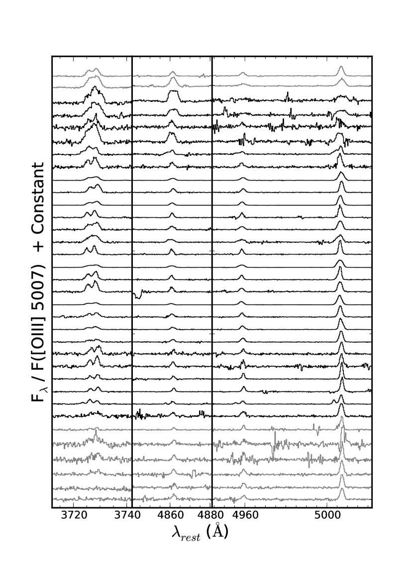
Figure 1.— The spectra of 34 galaxies with complete coverage of the R23 metallicity indicator ([O III]+ [O II]/ H$\beta$; Pagel et al. 1979) are shown. The spectra of 26 objects that comprise our MZ sample are shown in black, and are sorted by stellar mass with higher masses at the top (the same as their appearance in Tables 2 and 3). The two AGN candidates are shown in grey at the top, and also continue the mass-ordered scheme. The Class 3 objects with ambiguous optical counterparts are shown at the bottom (in grey) in the same order as their appearance in the tables. All spectra are normalized by their flux in [OIII] $\lambda 5007$, so it is apparent that higher mass galaxies have relatively stronger H$\beta$ and [O II] emission. The strong “absorption” trough near 4845 Å in one object (980802) is a detector artifact.

Because of the faintness of the emission lines, and the narrow bandpass in our search data, we use followup spectroscopy with DEIMOS (Faber et al., 2003) to identify the redshifts of the IMACS-detected galaxies. The primary goal of these observations was to confirm Ly$\alpha$ emitting galaxies and measure the faint-end slope of the Ly$\alpha$ luminosity function at $z=5.7$ (Henry et al., 2012). However, for the foreground galaxies at $z\sim 0.6-0.7$, these followup observations contain the [O III]$\lambda\lambda 4959,5007$, [O II]$\lambda\lambda 3727,3729$, and H$\beta$ emission lines that comprise the R23 metallicity indicator (Pagel et al., 1979). Three classes of these objects were included on followup slit-masks:

1. Emission line galaxies for which continuum in the search data ruled out the Ly$\alpha$ identification were chosen as MZ targets. To obtain the best possible spectrum, we searched the COSMOS photometric redshift catalog (Ilbert et al., 2009) for nearby galaxies ($<2$″) with $z\sim 0.6-0.7$, and shifted the slit-positions to coincide with these matches. In total, the final sample of 26 star forming galaxies (described in §3) contains 15 objects that meet these criteria.

2. Additionally, galaxies were drawn from the [O III] + H$\beta$ narrowband excess catalog which we derived in Dressler et al. (2011a). The present star-forming sample contains 11 objects that were selected in this way.

3. Finally, we also detect R23 from ultra-faint emission lines which we originally considered Ly$\alpha$ candidates, but, upon the followup observations described below, we determined that the discovery line was [O III]  $\lambda 4959$, [O III] $\lambda 5007$, or H$\beta$. Six galaxies with measurable R23 fall under this classification.

In practice, the objects described in #3 are difficult to evaluate; their imaged counterparts are sometimes ambiguous due to their faintness and uncertain position within the blind-search slit. Therefore, in this paper we focus on the former two classes. For completeness, in Tables 2 and 3 we list the subset of these objects where R23 could be measured; however, we do not consider them further in this paper.

The DEIMOS observations of these followup slit-masks were carried out in January 2011 and January 2012. A summary of observations for each followup mask is given in Table 1. In four of the five masks, we used slit-widths and PAs that were matched to the search data (1.5″ wide and 90° east of north). On mask L, in order to better locate objects detected through blind spectroscopy, we used a slit orientation which is orthogonal to the venetian blind search slits. This method also allowed for narrower slits (1.2″). All observations were carried out using the the GG495 blocking filter with 830G grating. Under this configuration, we achieved a spectral resolution of 3.7 Å  (2.9 Å) for a source that fills the 1.5″  (1.2″) slit. The grating angle was chosen to give a central wavelength of 7270 Å, with blue coverage down to 5500Å for most slits.

The DEIMOS spectra were reduced using the DEEP2 DEIMOS data reduction pipeline (Cooper et al., 2012), with an updated optical model for the 830G grating (P. Capak, private communication). The data were flux calibrated using observations of several spectrophotometric standard stars, taken through a 1.5″ slit at the parallactic angle. The stars used were G191B2B, GD50, Feige 66, Feige 67, and Hz 44 (Massey & Gronwall, 1990; Oke, 1990), and the data for each was taken from the ESO spectrophotometric standard star database. Sensitivity functions derived from these stars differ systematically between observations, with offsets up to 30%. After shifting the lower sensitivity functions to match the highest one, the observations agree at the 2-3% level, indicating an excellent relative calibration.

Finally, we have verified that the effects of differential atmospheric refraction have a negligible impact on our measured line flux ratios. In order to quantify possible differential slit losses, we calculate the component of the atmospheric refraction that falls perpendicular to the slit in each observation (frame) of each mask. The worst case occurs on mask L, where the slits are narrowest and the slit-PA was the furthest from parallactic. For these data, the refraction (perpendicular to the slit) between 6000 Å (near [O II]) and 8000 Å (near [O III] and H$\beta$) ranges from 0.04 to 0$\farcs$33 (Fillipenko, 1982). Therefore, since the guiding was done in the R-band (in between the observed wavelengths of the emission lines), we estimate the slit-losses on the red and blue parts of our spectra differ by no more than 4% (for 1″ seeing). In most frames, the effect is even smaller, so we conclude that no systematic correction is needed to interpret our emission line ratios.

2.2. COSMOS Imaging Data

In order to derive stellar masses (§3), we use the wide range of imaging data provided by the COSMOS team. A more detailed description of the catalogs can be found in Capak et al. (2007) and Ilbert et al. (2009). In summary, the photometric data include GALEX imaging, a wealth of ground-based, broad-band optical and near-infrared imaging, and the four Spitzer/IRAC bands. Furthermore, our SED fits are improved by the inclusion of intermediate-band imaging, and updated Subaru/SuprimeCam $z^{\prime}$-band data (from observations made with the new, fully depleted, red-efficient CCDs). Since the optical and near-infrared photometry are performed in 3″ apertures on data with homogenized PSFs (1.5″ FWHM), we apply a point source aperture correction of -0.28 magnitudes to all optical and near-infrared bands. For the IRAC data we use 3.8″ diameter apertures, and apply point source aperture corrections of -0.29, -0.33, -0.51, and -0.59 magnitudes to bands one through four. No aperture corrections are applied to the GALEX data, as these magnitudes were derived from fits to the PSF. Finally, we note that the recommended zero point offsets have been applied (Capak et al., 2007; Ilbert et al., 2009), and a Galactic foreground extinction correction is made using the Cardelli et al. (1989) extinction curve with E(B-V) = 0.019.

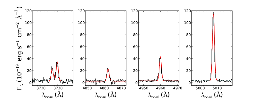
Figure 2.— The DEIMOS spectrum of object 54.5+4-0.18 measures the R23 oxygen abundance indicator with high signal to noise. The Gaussian fits used to measure the emission line fluxes are shown in red. From left to right, the lines shown are [O II] $\lambda\lambda 3727,3729$, H$\beta$, [O III] $\lambda 4959$, and [O III] $\lambda 5007$. This spectrum is representative of the fainter, lower mass galaxies in our sample (see Tables 2 and 3).

3. Analysis

3.1. Emission Line Measurements

In total, we identify 47 galaxies at $z\sim 0.6-0.7$; of these 34 have complete coverage of the R23 ([O III]+ [O II]/ H$\beta$; Pagel et al. 1979) metallicity indicator. Their spectra are shown in Figure 1. The remaining 13 galaxies at these redshifts either have essential lines lost in the OH airglow spectrum, or are class #3 objects (described above), where the observed spectrum is especially faint because the galaxy may not be centered in the slit. Only six class #3 objects (without mass measurements) have R23 measurements; their spectra are shown in grey at the bottom of Figure 1. Excluding these objects leaves 28 galaxies with both mass and R23 constraints. In §3.3 we show that two of these galaxies may contain active nuclei, so we adopt a final sample that includes the remaining 26 star-forming objects.

Emission line fluxes are measured for all of the $z\sim 0.6-0.7$ galaxies that we identified. Gaussian profiles are fit to each line, and uncertainties are determined through a Monte Carlo simulation where noise is added to the spectrum and the fits are repeated. For [O II], the two doublet components are fit simultaneously. As an example, Figure 2 shows a typical spectrum and the Gaussian fits to the emission lines.

To facilitate a correction for H$\beta$ stellar absorption, we also measure emission line equivalent widths. Because it can be difficult to assess the uncertainty on the continuum flux density when it is measured spectroscopically, we compare two methods. On one hand, we measure the equivalent widths directly from the spectra. In 25/28 objects in our sample, we detect continuum, although it is sometimes weak. As a second method, we compare the emission line fluxes from the DEIMOS data to the continuum under the emission line from the SED fit (described below). After accounting for a systematic offset (because the emission line fluxes are subject to slit losses but the SED fits use total fluxes), the equivalent widths measured by these different techniques agree to within 50%. We adopt this level of uncertainty on the H$\beta$  equivalent widths.

Finally, having measured the fluxes and equivalent widths of our emission lines, we apply a correction for the stellar absorption. Because the stellar absorption component is much broader than the emission line, this correction depends on the spectral resolution. At the resolution of our data, the correction is approximately 1 Å  in equivalent width (Cowie & Barger, 2008; Zahid et al., 2011). While the amount of absorption also depends slightly on the age of the stellar population, the main source of uncertainty in this correction is from the observed H$\beta$  emission equivalent width, as discussed above. We propagate this error in our H$\beta$ fluxes and the metallicities that we infer in §4.

3.2. Stellar Masses, SFRs, and dust constraints from SED fitting

Stellar masses are determined by fitting template stellar populations to the broad- and intermediate-band photometry described in §2. For this task, we use FAST (Fitting and Assessment of Synthetic Templates; Kriek et al. 2009). The choice of population synthesis templates can have an important impact on the properties derived from SEDs, because the contribution from the (infrared-bright) thermally pulsing asymptotic giant branch (TP-AGB) stars differs from model to model. The most widely used templates are Bruzual & Charlot (2003; BC03), Maraston (2005), and Charlot & Bruzual (2007; Bruzual 2007); the latter two options provide a larger contribution from TP-AGB stars (and correspondingly smaller masses). Nevertheless, the proper contribution from TP-AGB stars remains a subject of debate (Kriek et al., 2010; Conroy & Gunn, 2010; Zibetti et al., 2013). Therefore, in order to facilitate comparisons with the literature, we derive stellar masses using the BC03 models. We have verified that the Charlot & Bruzual and Maraston et al. models produce stellar masses that are systematically smaller by approximately 0.1 dex.

In order to assure accurate stellar population constraints, it is also important to account for emission line contribution to our SEDs. (The stellar synthesis templates that we fit to the SEDs do not contain nebular features. Failing to remove emission line contamination can result in incorrectly inferred ages and stellar masses; Schaerer & de Barros 2009; Atek et al. 2011.) We use our line fluxes to calculate the small contribution from [O II] to the $r$-band, and [O III] and H$\beta$ to the $i$-band. For the galaxies in our sample, we find that 1-5% of the $r-$ band light and 2-15% of the $i-$band light can be attributed to emission lines. These contributions are subtracted from the $r$ and $i-$ band continuum flux densities. Emission from H$\alpha$, on the other hand, falls between the $z^{\prime}$ and $J$ bands, so it does not contaminate any of the photometry in the present analysis. Finally, we consider emission line contamination to the intermediate band photometry. In these cases, the corrections will be larger and more uncertain. Therefore, we exclude the band at 624 nm that includes [O II], and the band at 827 nm that covers [O III] and H$\beta$. The remaining ten intermediate bands should be relatively unaffected.

The grid of stellar population parameters that we fit with FAST include: a set of exponentially declining star formation histories with e-folding times, $\tau$, ranging from 40 Myr to 10 Gyr; characteristic stellar population ages ranging from 50 Myr to the age of the universe at $z\sim 0.6-0.7$; and $A_{V}=0-3$ for a Calzetti et al. (2000) extinction curve. Additionally, we use a Chabrier (2003) IMF with metallicities of 0.004, 0.008, and 0.02 (solar). Supersolar metallicities are excluded, because, as we will show in §4, the galaxies in our sample mostly have subsolar to solar gas-phase metallicities. The derived stellar masses, SFRs, and visual extinction values are given in Table 3. Because of the intermediate band photometry, the dust extinction constraints exclude much of the allowed parameter space. Therefore we use the SED-derived dust constraints to correct our emission line ratios, including these uncertainties in our error budget. In making this correction, we also account for the fact that nebular extinction is 2.3 times higher than stellar extinction on average (Calzetti et al., 2000; Cresci et al., 2012). While the precise relation between stellar and nebular extinction remains controversial (Cowie & Barger, 2008; Cresci et al., 2012; Wofford et al., 2013), we adopt the “standard” Calzetti et al. (2000) relation to allow comparison with other studies.

In §6 and 7 we draw conclusions based on the SFRs that we have derived from these SED fits. In order to verify that the SFRs are reliable, we have carried out an assessment of the systematic uncertainties by comparing SFRs derived from [O II], H$\beta$, and the SED fits. The results, outlined in the Appendix, show that the agreement between the different diagnostics is good; systematic offsets are smaller than 0.2 dex. This level of uncertainty does not affect our conclusions.

3.3. Contamination from AGN

In order to measure the MZ relation of star-forming galaxies, it is important to ensure that the observed emission lines do not originate from an active galactic nucleus (AGN). The typical approach for low redshift galaxies is to use the [O III]/ H$\beta$ and [N II]/ H$\alpha$ emission line ratios (the canonical BPT diagram; Baldwin, Phillips, & Terlevich 1981). However, for the redshift of our sample, H$\alpha$ and [N II] fall at infrared wavelengths. Therefore, in lieu of followup spectroscopy, we turn to an alternate diagnostic: the Mass-Excitation (MEx) diagram (Juneau et al., 2011). This approach, shown in Figure 3, uses stellar mass as a proxy for the H$\alpha$/[N II] $\lambda 6583$ ratio (relying on the MZ relation). The resulting diagram appears qualitatively similar to the traditional BPT diagram, with AGN falling towards the top and right of the plot. In this figure, the data for our galaxies (red points) are compared to that from the SDSS (contours), and the solid black line demarcates the difference between star-forming galaxies, AGN, and composite objects (as defined by Juneau et al. 2011). While the evolution of MZ relation compromises somewhat the use of this method, we note that two of our galaxies are found in the area identified as possible AGN. Since metallicity evolution works in the sense of shifting the proxy relation between H$\alpha$/[N II] $\lambda 6583$ and mass, it shifts the star-forming locus (and black threshold curves) to the right in Figure 3. Therefore, the two objects in the AGN or composite part of the sample may in fact be part of the non-AGN distribution; however, we take the conservative step of excluding them from further analysis. We list the measured and derived properties of the two candidate AGN at the ends of Tables 2 and 3.

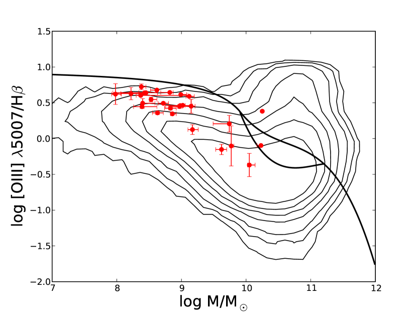
Figure 3.— The [O III] / H$\beta$ ratio as a function of stellar mass can be used to identify AGN, similar to the [O III]/ H$\beta$ vs. [N II]/ H$\alpha$ “BPT” diagram (Baldwin, Phillips, & Terlevich, 1981; Juneau et al., 2011). Red point show our emission line selected sample, while contours (with levels defined arbitrarily) show the SDSS data. The solid black lines show the demarcation between star-forming galaxies (below and to the left), objects with active nuclei (above and to the right), and composite objects (the region in between the black lines around $10^{10}$- $10^{11}$ M_☉). The two highest mass objects in our sample, 55.5-3-0.60 and 73.5+5-0.54, fall outside of the $z=0$ star-forming locus, so we identify them as candidate AGN.

4. Calculating oxygen Abundances

Interpreting metal abundance measurements requires that we account for systematic uncertainties. Different methods for measuring strong oxygen abundances yield results which are offset by up to 0.7 dex (Kewley & Ellison, 2008; López-Sánchez et al., 2012; Andrews & Martini, 2013). On one hand, photoionization models that are used to derive theoretical calibrations (i.e. Kewley & Dopita 2002) are often based on simplistic assumptions about H II region geometries and ionizing spectra (van Zee et al., 2006). On the other hand, empirical methods, which correlate line ratios with H II region electron temperatures (i.e. Pettini & Pagel 2004; Pilyugin & Thuan 2005), generally give lower metallicities than photoionization model-based calibrations (McGaugh, 1991; Kewley & Dopita, 2002). Because electron temperature measurements may be overestimated when temperature and density gradients are present in H II regions, it is possible that the empirical calibrations are biased towards low metallicities (Peimbert & Costero, 1969; Stasińska, 2005). Alternatively, Nicholls et al. (2012) have suggested that discrepancies between electron-temperature measurements and theoretical strong-line estimates can be explained if the electrons in H II regions deviate from an equilibrium Maxwell-Boltzmann distribution.

Ultimately, the differences between metallicity calibrations are still not fully understood, but the systematic offsets can be accounted for using a set of transformation equations given by Kewley & Ellison (2008). In the sections that follow (except for §6), we use the calibration from Kobulnicky & Kewley (2004; hereafter KK04), which is the mean of two theoretical R23 calibrations in the literature (McGaugh 1991 and Kewley & Dopita 2002). In §6 we instead use the calibration from Maiolino et al. (2008) so that we may compare our data to results from Mannucci et al. (2011).

4.1. High-Metallicity or Low? Determining the Branch of R23

Metallicities derived from R23 can be degenerate, since this diagnostic is double valued. At high metallicities, the oxygen lines are weaker because cooling is efficient and the H II regions have lower electron temperatures. On the other hand, at low metallicities, the overall decrease in oxygen relative to hydrogen also imprints a decrease in R23 with decreasing metallicity. The “turnover” metallicity that demarcates the transition between the upper and lower branches of R23 depends on the ionization parameter, and differs among the calibrations that are in the literature. For the typical ionization parameters of our galaxies, and the KK04 calibration, the turnover metallicity is around 12+log(O/H) $\sim 8.4$, which is reached when log(R23)$\sim 0.9-1.0$.

Many different methods have been suggested for breaking the degeneracy between the upper and lower branch. The most rigorous of these is to compare to an alternative metallicity diagnostic. Kewley & Ellison (2008) advocate for the use of the [N II] $\lambda 6583$/[O II]  or [N II] $\lambda 6583$ /H$\alpha$ ratios to first provide a metallicity estimate that identifies the branch. However, this method is more challenging at $z>0.5$ (requiring infrared spectroscopy to reach very faint [N II] $\lambda\lambda 6548,6583$ lines), and impossible from the ground at $z>2$. The R23 diagnostic, on the other hand, can be measured from the ground out to $z\sim 3$ (Maiolino et al., 2008). It is therefore imperative that we learn how to break the R23-metallicity degeneracy without observations of the [N II] $\lambda\lambda 6548,6583$ lines. Here, we examine other methods for establishing the R23-branch that have been proposed in the literature.

In Figure 4 we investigate the branch of R23 by plotting four different diagnostics as a function of stellar mass. For comparison, we show the four H$\beta$-detected galaxies ($0.60<z<0.85$) from the PEARS Survey (Probing Evolution and Reionization Spectroscopically; Xia et al. 2012). In the upper left panel, we show that R23 decreases with increasing stellar mass for most of our sample. Furthermore, three of the four galaxies from Xia et al. follow the trends from our emission line selected sample. This diagnostic paints a clear picture: if metallicity decreases as a function of decreasing mass, most of the galaxies in our sample must fall on the upper branch of the R23 indicator. The two lowest mass galaxies shown in Figure 4 (1217842 from our sample, and 246 from Xia et al.) hint at a possible turnover at $M\sim 8.0-8.5$, indicating that these galaxies may fall on the lower branch of R23.

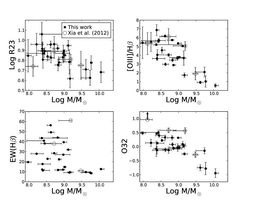
Figure 4.— Our measured values of R23 decrease with increasing stellar mass, implying that most of the galaxies in our sample fall on the upper branch of R23. This diagram is contrasted with three other diagnostics that have previously been used to identify whether galaxies have low or high metallicities (Maiolino et al., 2008; Hu et al., 2009; Xia et al., 2012). These include the [O III]$\lambda\lambda 4959,5007$ / H$\beta$ flux ratio, the rest-frame equivalent width of H$\beta$, and the ratio O32 $\equiv$ log ([O III]$\lambda\lambda 4959,5007$ / [O II] $\lambda\lambda 3726,3729$). With an H$\beta$ EW of 352Å  (rest), object 246 from Xia et al. is not shown in the EW(H$\beta$) panel.

Because it is not ideal to introduce a mass dependence on our metallicity derivations, we explore other emission line diagnostics in Figure 4. First, we compare to the emission line ratios of [O III]/H$\beta$ and log([O III]/ [O II]) $\equiv$ O32 as a function of stellar mass. These line ratios have been proposed to break the R23 degeneracy by Maiolino et al. (2008), with low metallicity solutions being preferred when [O III]/H$\beta$$>5$ and O32 $>0.5$. Indeed, Figure 4 shows that the galaxies above these thresholds also prefer to have higher values of R23 (and lower metallicities on the upper branch). Nevertheless, we still see very little evidence for a substantial population of galaxies extending to metallicities below the R23 turnaround. The only object that passes both the O32 and [O III]/H$\beta$ thresholds is object 246 from Xia et al. (2012).

The inference of upper branch metallicities for 3/4 of the objects presented by Xia et al. (2012) contrasts with their lower branch assumption. These authors argued for lower metallicities because of the relatively high values of [O III]/H$\beta$ and O32 for most of their sample. However, comparison to the R23 vs mass plot (upper left) shows that for at least three of these galaxies, higher metallicity solutions are more plausible. (Although the galaxies presented by Xia et al. 2012 may prefer higher O32 and ionization parameters than the remainder of our sample, metallicity is not a strong function of ionization parameter on the upper branch, so their galaxies still follow our R23-stellar mass correlation.)

Ultimately, caution is required when using [O III]/H$\beta$ and O32 to determine the branch of R23, because these quantities are dependent on the ionization parameter. Observations of high-redshift galaxies show that their line ratios are offset to high values of [O III]/H$\beta$ at a fixed [N II]/H$\alpha$ (Shapley et al., 2005; Erb et al., 2006; Hainline et al., 2009). This offset is usually interpreted as evidence for a systematically high ionization parameter (Brinchmann et al., 2008), suggesting that some galaxies deviate from the local metallicity vs. ionization parameter correlation. In summary, attempting to break the R23 degeneracy using quantities that depend on the ionization parameter could erroneously indicate lower branch solutions.

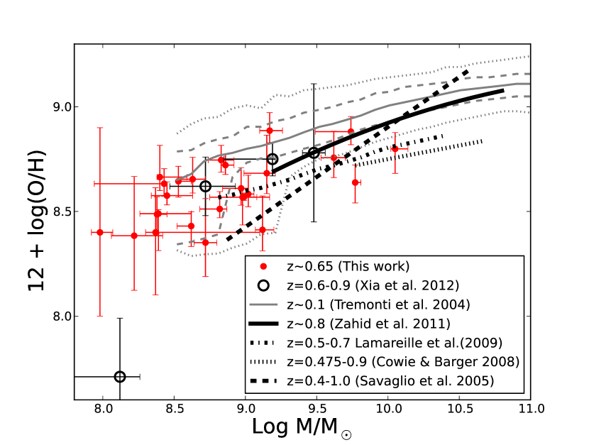
Figure 5.— The addition of our 26 low mass galaxies constrains the low mass portion of the MZ relation at intermediate redshifts. For comparison, we have re-calculated the metallicities presented in Xia et al. (2012), assuming– contrary to these authors– that the three highest mass objects have metallicities on the upper branch. Other studies are shown for comparison, and are (when necessary) converted to a Chabrier (2003) initial mass function and a Kobulnicky & Kewley (2004) metallicity. The dashed and dotted grey lines that follow the Tremonti et al. (2004) MZ relation show the 68 and 95% contours for the SDSS data. For reference, solar metallicity is 12 + log (O/H) = 8.69 (Allende Prieto et al., 2001).

In Figure 4, we also investigate the use of H$\beta$ equivalent width to select low-metallicity galaxies. Kakazu et al. (2007) and Hu et al. (2009) have found that, for their emission line selected sample, galaxies are likely to have very low metallicities (indicated by detectable [O III] $\lambda$4363 emission) when their H$\beta$ equivalent widths are more than 30 Å (rest). However, 8/26 galaxies in our sample meet this criterion, and we do not detect [O III] $\lambda 4363$ in any objects. What is more apparent in Figure 4, is that a cut in H$\beta$ equivalent width merely selects against galaxies with $M\gtrsim 10^{9.0}$ $M_{\sun}$. As we show in §5, the Hu et al. sample has, on average, higher H$\beta$ equivalent widths and somewhat lower luminosities than the present sample of emission line objects. We infer that it is not straightforward to use H$\beta$ equivalent width to discriminate between upper and lower branch metallicities.

Guided by Figure 4 we conclude that, in the absence of other metallicity diagnostics, the correlation between stellar mass and R23 is the preferred method to break the R23-degeneracy. This exercise shows that for $z\sim 0.6-0.7$ galaxies, the maximum value of R23 is reached between $10^{8.0}$ and $10^{8.5}$ M_☉. Therefore, we adopt upper branch solutions above $M=10^{8.2}$ $M_{\sun}$. The two lowest mass galaxies (1217842 from our sample and 246 from Xia et al. 2012) are less certain. For 1217842 we adopt a metallicity in the turn around region (12 + log(O/H) = 8.4), with error bars denoting the upper bound of the high metallicity solution and the lower bound of the low metallicity solution. The lowest-mass object from Xia et al. (#246) is tentatively assigned to the lower branch because of its more extreme line ratios, although we caution that the H$\beta$ measurement could be in error because it is blended with [O III] in their low resolution data. Followup spectroscopy can better constrain the metallicities of galaxies near the R23 turnaround by providing the [N II]/H$\alpha$ and [N II]/[O II] ratios (Kewley & Ellison, 2008). At present, however, the conclusions drawn in the remainder of this work do not depend on these two galaxies because their metallicity errors are large. Oxygen abundances for the entire sample are listed in Table 3.

Our inference of upper branch metallicities at $M>10^{8.2-8.5}M_{\sun}$ is inconsistent with results reported by Zahid et al. (2011). In contrast to Figure 4, Zahid et al. find that the mean value of R23 turns over around $M\sim 10^{9.2}$ M_☉ for their $z\sim 0.8$ sample. They interpret the turnover as evidence for lower branch metallicities. However, as can be seen in their Figure 4, the data are increasingly noisy below $M<10^{9.5}$ M_☉, and objects with R23 $>10$ have been removed as candidate AGN. The coupling of these effects may bias the lowest mass bin towards lower mean values of R23, and mimic the effect of a turnover in the R23 vs mass correlation. We conclude that on average, galaxies at $z\sim 0.6-0.7$ fall on the upper branch of R23 for $M\gtrsim 10^{8.2-8.5}M_{\sun}$. At higher redshifts, where metallicity evolution is significant (i.e. Erb et al. 2006), we expect that the transition from the upper to lower branch of R23 will occur at higher stellar masses.

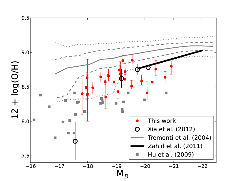
Figure 6.— The luminosity metallicity relation for the present emission line selected sample is compared to correlations from the literature. Notably, we compare to the measurements of the ultra-strong emission line galaxies reported by Hu et al. (2009). Because these galaxies have detected [O III] $\lambda$ 4363 Å emission, we assume that they fall on the lower branch of R23. Their metallicities are recalculated using the KK04 calibration (assuming no dust, as justified by Hu et al.).

Table 2Emission Line Measurements

IMACS ID	COSMOS ID	RA	Dec	$z$	F([O III] $\lambda$5007)	F([O III]  $\lambda$4959)	F(H$\beta$)	F([O II] $\lambda 3727$)	EW(H$\beta$)
		(J2000)	(J2000)						Å (rest)
27.5+5-0.47	799604	10:00:11.314	+02:04:07.60	0.675	$16.7\pm 6.3$	$\cdots$	$39.2\pm 0.7$	$53.9\pm 1.3$	12.7
99.5-3-0.84	1235118	10:00:53.842	+02:22:06.88	0.685	$19.75pm12.7$	$\cdots$	$25.1\pm 0.6$	$58.0\pm 1.2$	8.5
90.5+6-0.63	1265343	10:00:09.101	+02:19:52.02	0.678	$10.2\pm 2.7$	$\cdots$	$6.3\pm 0.3$	$16.4\pm 0.4$	9.2
100.5-2-0.41	1234271	10:00:50.551	+02:22:22.66	0.683	$13.4\pm 2.2$	$\cdots$	$19.0\pm 0.4$	$48.5\pm 0.9$	9.7
65.5-1-0.69	1003946	10:00:47.710	+02:13:36.83	0.620	$26.0\pm 0.4$	$\cdots$	$19.4\pm 3.0$	$40.9\pm 0.7$	9.6
87.5+4-0.86	1242162	10:00:18.502	+02:19:06.82	0.656	$15.4\pm 0.7$	$5.4\pm 0.4$	$5.4\pm 1.2$	$19.4\pm 0.8$	9.2
95.5+4-0.94	1236769	10:00:21.331	+02:21:05.22	0.667	$158.5\pm 1.4$	$52.5\pm 0.5$	$40.8\pm 0.5$	$112.3\pm 1.0$	32.0
35.5+5-0.23	794540	10:00:09.038	+02:06:08.16	0.620	$57.0\pm 0.4$	$19.1\pm 0.4$	$19.6\pm 0.5$	$70.5\pm 1.0$	14.8
$\cdots$	1015084	10:00:41.863	+02:09:12.66	0.678	$309.7\pm 0.9$	$104.1\pm 0.5$	$75.1\pm 0.4$	$200.3\pm 1.0$	39.5
54.5+6-0.09	1036285	10:00:01.553	+02:10:51.89	0.684	$53.3\pm 1.0$	$17.2\pm 0.6$	$18.5\pm 0.3$	$49.6\pm 0.6$	27.0
25.5+7-0.08	801017	09:59:58.039	+02:03:38.89	0.638	$36.9\pm 0.4$	$12.8\pm 0.4$	$13.2\pm 0.8$	$46.9\pm 1.0$	12.1
23.5+2-0.33	775548	10:00:32.287	+02:03:09.25	0.670	$32.8\pm 0.7$	$12.2\pm 1.3$	$14.8\pm 0.5$	$44.8\pm 1.1$	22.3
$\cdots$	1035959	09:59:59.347	+02:10:57.10	0.628	$35.2\pm 0.3$	$12.7\pm 0.2$	$13.2\pm 0.7$	$34.7\pm 0.6$	11.7
$\cdots$	982000	10:01:07.140	+02:12:08.99	0.621	$235.1\pm 0.6$	$77.2\pm 0.5$	$53.3\pm 0.7$	$112.7\pm 0.9$	44.0
$\cdots$	1013478	10:00:18.701	+02:09:41.74	0.635	$34.9\pm 0.3$	$12.1\pm 0.3$	$11.2\pm 0.5$	$40.7\pm 0.6$	28.4
$\cdots$	980802	10:01:07.135	+02:12:38.22	0.621	$27.3\pm 0.4$	$9.2\pm 0.6$	$11.9\pm 0.7$	$40.5\pm 0.7$	49.3
28.0+7.1	799190	10:00:03.035	+02:04:13.98	0.638	$167.5\pm 0.6$	$57.3\pm 0.4$	$35.2\pm 0.8$	$91.3\pm 1.0$	56.3
$\cdots$	770439	10:00:42.334	+02:05:43.53	0.629	$34.4\pm 0.4$	$11.5\pm 0.4$	$9.8\pm 0.7$	$23.9\pm 0.8$	22.9
$\cdots$	1009808	10:00:44.558	+02:11:18.04	0.616	$96.9\pm 0.4$	$32.5\pm 0.5$	$22.2\pm 0.9$	$45.2\pm 0.8$	38.0
$\cdots$	1237667	10:00:52.368	+02:20:58.18	0.640	$59.2\pm 0.4$	$21.2\pm 0.4$	$13.6\pm 0.4$	$24.9\pm 1.0$	40.9
$\cdots$	772773	10:00:25.567	+02:04:44.36	0.616	$21.5\pm 0.5$	$8.2\pm 0.8$	$6.9\pm 1.0$	$22.3\pm 1.0$	11.3
48.5-4-0.66	989316	10:01:08.537	+02:09:21.70	0.674	$13.8\pm 0.5$	$4.7\pm 1.0$	$4.96\pm 0.2$	$16.1\pm 0.7$	17.7
54.5+4-0.18	1010994	10:00:16.097	+02:10:51.60	0.634	$28.7\pm 0.2$	$10.0\pm 0.3$	$5.4\pm 0.5$	$13.4\pm 0.5$	12.2
47.5+3-0.85	1015516	10:00:27.792	+02:09:06.43	0.679	$34.1\pm 0.3$	$12.4\pm 0.2$	$8.5\pm 0.2$	$17.7\pm 0.6$	43.5
$\cdots$	1010583	10:00:21.408	+02:11:00.43	0.639	$45.2\pm 1.5$	$14.6\pm 0.8$	$10.6\pm 2.1$	$28.5\pm 0.6$	27.9
$\cdots$	1217842	10:00:54.658	+02:19:01.81	0.633	$21.4\pm 0.3$	$8.4\pm 0.4$	$5.1\pm 1.7$	$9.8\pm 0.8$	19.6
Objects lacking clear optical counterparts in the COSMOS data
52.5+8-0.69	$\cdots$	09:59:51.374	+02:10:23.28	0.678	$15.6\pm 0.8$	$3.7\pm 0.9$	$2.1\pm 0.1$	$3.6\pm 0.4$	$\cdots$
45.5+7-0.25	$\cdots$	09:59:55.699	+02:08:38.51	0.678	$\cdots$	$2.2\pm 0.7$	$2.6\pm 0.4$	$9.6\pm 1.0$	6.5
46.5-7-0.04	$\cdots$	10:01:25.152	+02:08:52.34	0.672	$6.2\pm 0.5$	$2.5\pm 1.5$	$2.4\pm 0.8$	$5.4\pm 0.7$	$\cdots$
65.5-2-0.14	$\cdots$	10:00:50.904	+02:13:36.52	0.624	$14.1\pm 0.3$	$5.0\pm 0.9$	$5.4\pm 0.2$	$6.8\pm 0.8$	$\cdots$
47.5+6-0.90	$\cdots$	10:00:07.145	+02:09:07.81	0.639	$14.4\pm 0.4$	$5.0\pm 3.8$	$3.4\pm 0.8$	$<9.5$	$\cdots$
87.5-1-0.06	$\cdots$	10:00:48.792	+02:19:06.54	0.620	$15.4\pm 0.3$	$5.3\pm 1.6$	$6.0\pm 1.7$	$1.9\pm 1.3$	$\cdots$
Candidate AGN
55.5-3-0.60	984577	10:01:01.126	+02:11:07.85	0.623	$39.5\pm 0.4$	$13.7\pm 0.4$	$16.4\pm 0.5$	$51.6\pm 0.7$	9.9
73.5+3-0.54	998509	10:00:25.046	+02:15:38.15	0.642	$38.7\pm 0.5$	$12.4\pm 0.6$	$48.4\pm 0.8$	$93.3\pm 0.9$	9.4

Note. — Emission line fluxes are in units of 10^-18 erg s^-1 cm^-2. Equivalent widths and H$\beta$ fluxes are given as measured (without applying the 1Å stellar absorption correction.) Objects lacking an IMACS ID were selected strictly from the COSMOS narrowband (NB816) imaging, as we described in §2. The [O II] flux is the sum of the $\lambda\lambda 3726,3729$ doublet fluxes. In six cases, one of the lines in the [O III] doublet lines fell on an OH sky line; in this situation, metallicities are derived by assuming a flux ratio of F([O III] $\lambda$5007)/ F([O III] $\lambda$4959) $\equiv 3$.

Table 3Derived Properties

IMACS ID	COSMOS ID	$M_{B}$	$U-B$	log M∗	log SFR	$A_{V}$	log R23	log O32	12+log(O/H)	log $q$
27.5+5-0.47	799604	-20.93	0.52	$10.05^{+0.09}_{-0.03}$	$1.23_{-0.21}^{+0.34}$	$1.80^{+0.13}_{-0.48}$	$0.68\pm 0.10$	$-0.94\pm 0.16$	$8.80_{-0.12}^{+0.08}$	$7.00_{-0.13}^{+0.09}$
99.5-3-0.84	1235118	-20.71	0.45	$9.77^{+0.04}_{-0.00}$	$0.95_{-0.00}^{+0.20}$	$1.40^{+0.08}_{-0.19}$	$0.77\pm 0.07$	$-0.78\pm 0.22$	$8.63_{-0.10}^{+0.08}$	$7.05_{-0.10}^{+0.14}$
90.5+6-0.63	1265343	-19.24	0.61	$9.74^{+0.00}_{-0.25}$	$-0.54_{-0.00}^{+0.12}$	$0.20^{+0.30}_{-0.05}$	$0.63\pm 0.08$	$-0.14\pm 0.11$	$8.88_{-0.06}^{+0.07}$	$7.65_{-0.07}^{+0.12}$
100.5-2-0.41	1234271	-20.39	0.42	$9.62^{+0.08}_{-0.09}$	$0.62_{-0.05}^{+0.38}$	$1.00^{+0.28}_{-0.31}$	$0.71\pm 0.10$	$-0.75\pm 0.19$	$8.76_{-0.10}^{+0.13}$	$7.11_{-0.10}^{+0.06}$
65.5-1-0.69	1003946	-19.56	0.42	$9.17^{+0.09}_{-0.07}$	$-0.45_{-0.06}^{+0.44}$	$0.60^{+0.07}_{-0.21}$	$0.62\pm 0.09$	$-0.26\pm 0.05$	$8.89_{-0.06}^{+0.09}$	$7.55_{-0.11}^{+0.09}$
87.5+4-0.86	1242162	-19.15	0.44	$9.15^{-0.06}_{-0.16}$	$-0.42_{-0.00}^{+0.07}$	$0.00^{+0.18}_{-0.00}$	$0.78\pm 0.12$	$0.03\pm 0.04$	$8.68_{-0.10}^{+0.18}$	$7.66_{-0.12}^{+0.14}$
95.5+4-0.94	1236769	-20.08	0.37	$9.12^{+0.08}_{-0.05}$	$0.30_{-0.22}^{+0.59}$	$0.60^{+0.27}_{-0.40}$	$0.85\pm 0.05$	$0.09\pm 0.10$	$8.41_{-0.10}^{+0.16}$	$7.57_{-0.12}^{+0.14}$
35.5+5-0.23	794540	-19.89	0.30	$9.02^{+0.04}_{-0.04}$	$0.02_{-0.05}^{+0.22}$	$0.20^{+0.40}_{-0.07}$	$0.85\pm 0.06$	$-0.03\pm 0.07$	$8.58_{-0.06}^{+0.09}$	$7.56_{-0.12}^{+0.07}$
$\cdots$	1015084	-20.26	0.21	$8.99^{+0.09}_{-0.00}$	$0.33_{-0.00}^{+0.15}$	$0.00^{+0.09}_{-0.00}$	$0.89\pm 0.01$	$0.32\pm 0.02$	$8.57_{-0.02}^{+0.01}$	$7.83^{+0.02}_{-0.03}$
54.5+6-0.09	1036285	-18.93	0.40	$8.98^{+0.19}_{-0.23}$	$0.08_{-0.46}^{+0.38}$	$0.60^{+0.44}_{-0.60}$	$0.87\pm 0.08$	$-0.03\pm 0.14$	$8.57_{-0.13}^{+0.02}$	$7.54^{+0.14}_{-0.05}$
25.5+7-0.08	801017	-19.31	0.37	$8.97^{+0.05}_{-0.03}$	$-0.06_{-0.25}^{+0.00}$	$0.20^{+0.22}_{-0.20}$	$0.83\pm 0.06$	$-0.04\pm 0.06$	$8.61_{-0.08}^{+0.10}$	$7.56_{-0.08}^{+0.09}$
23.5+2-0.33	775548	-19.32	0.34	$8.86^{+0.06}_{-0.03}$	$-0.33_{-0.16}^{+0.18}$	$0.20^{+0.14}_{-0.20}$	$0.78\pm 0.04$	$-0.06\pm 0.05$	$8.72_{-0.04}^{+0.05}$	$7.61_{-0.08}^{+0.09}$
$\cdots$	1035959	-19.11	0.37	$8.83^{+0.09}_{-0.09}$	$-0.36_{-0.18}^{+0.20}$	$0.20^{+0.23}_{-0.20}$	$0.75\pm 0.06$	$0.08\pm 0.06$	$8.75_{-0.06}^{+0.07}$	$7.74_{-0.11}^{+0.10}$
$\cdots$	982000	-19.54	0.25	$8.82^{+0.05}_{-0.14}$	$0.43_{-0.48}^{+0.23}$	$0.40^{+0.24}_{-0.26}$	$0.92\pm 0.03$	$0.32\pm 0.08$	$8.51_{-0.04}^{+0.08}$	$7.80_{-0.10}^{+0.15}$
$\cdots$	1013478	-18.64	0.36	$8.72^{+0.08}_{-0.08}$	$-0.28_{-0.15}^{+0.54}$	$0.60^{+0.46}_{-0.24}$	$0.96\pm 0.08$	$-0.12\pm 0.11$	$8.35_{-0.16}^{+0.21}$	$7.40_{-0.05}^{+0.09}$
$\cdots$	980802	-18.74	0.37	$8.63^{+0.09}_{-0.08}$	$-0.56_{-0.50}^{+0.33}$	$0.20^{+0.27}_{-0.20}$	$0.83\pm 0.05$	$-0.11\pm 0.07$	$8.65_{-0.07}^{+0.10}$	$7.53_{-0.07}^{+0.11}$
28.0+7.1	799190	-19.07	0.24	$8.62^{+0.00}_{-0.10}$	$-0.04_{-0.20}^{+0.46}$	$0.20^{+0.43}_{-0.07}$	$0.96\pm 0.03$	$0.33\pm 0.07$	$8.43_{-0.10}^{+0.07}$	$7.77_{-0.13}^{+0.07}$
$\cdots$	770439	-18.46	0.36	$8.53^{+0.10}_{-0.00}$	$-1.08_{-0.00}^{+0.46}$	$0.20^{+0.11}_{-0.20}$	$0.84\pm 0.04$	$0.22\pm 0.04$	$8.64_{-0.08}^{+0.07}$	$7.80_{-0.07}^{+0.06}$
$\cdots$	1009808	-18.62	0.28	$8.45^{+0.18}_{-0.11}$	$-0.13_{-0.35}^{+0.18}$	$0.20^{+0.27}_{-0.20}$	$0.89\pm 0.03$	$0.39\pm 0.07$	$8.57_{-0.04}^{+0.07}$	$7.91_{-0.07}^{+0.11}$
$\cdots$	1237667	-17.99	0.30	$8.43^{+0.01}_{-0.49}$	$-0.51_{-0.02}^{+0.76}$	$0.00^{+0.82}_{-0.00}$	$0.87\pm 0.04$	$0.51\pm 0.08$	$8.63_{-0.06}^{+0.07}$	$8.05_{-0.27}^{+0.13}$
$\cdots$	772773	-18.72	0.28	$8.40^{+0.19}_{-0.02}$	$-0.61_{-0.02}^{+0.30}$	$0.00^{+0.15}_{-0.00}$	$0.81\pm 0.08$	$0.12\pm 0.04$	$8.66_{-0.06}^{+0.15}$	$7.72_{-0.06}^{+0.08}$
48.5-4-0.66	989316	-17.94	0.35	$8.39^{+0.23}_{-0.13}$	$-0.21_{-0.52}^{+0.37}$	$0.60^{+0.40}_{-0.60}$	$0.89\pm 0.09$	$-0.13\pm 0.14$	$8.49_{-0.18}^{+0.02}$	$7.44_{-0.18}^{+0.03}$
54.5+4-0.18	1010994	-18.18	0.40	$8.38^{+0.07}_{-0.00}$	$-1.41^{+0.06}_{-0.01}$	$0.00^{+0.04}_{-0.00}$	$0.92\pm 0.06$	$0.46\pm 0.02$	$8.49_{-0.09}^{+0.08}$	$7.91^{+0.05}_{-0.05}$
47.5+3-0.85	1015516	-17.82	0.36	$8.37^{+0.73}_{-0.07}$	$0.46_{-1.11}^{+0.30}$	$1.60^{+0.30}_{-1.54}$	$1.06\pm 0.12$	$-0.08\pm 0.25$	$8.40_{-0.30}^{+0.21}$	$7.36^{+0.22}_{-0.19}$
$\cdots$	1010583	-18.00	0.26	$8.22^{+0.20}_{-0.16}$	$-0.06_{-0.66}^{+0.28}$	$0.60^{+0.38}_{-0.56}$	$0.96\pm 0.11$	$0.13\pm 0.13$	$8.38_{-0.26}^{+0.28}$	$7.60^{+0.15}_{-0.17}$
$\cdots$	1217842	-18.00	0.20	$7.98^{+0.09}_{-0.06}$	$-0.48_{-0.32}^{+0.17}$	$0.00^{+0.22}_{-0.00}$	$0.85\pm 0.16$	$0.49\pm 0.05$	$8.40^{+0.50}_{-0.40}$	$8.05_{-0.27}^{+0.22}$
Objects with ambiguous counterparts in the COSMOS data
52.5+8-0.69	$\cdots$	$\cdots$	$\cdots$	$\cdots$	$\cdots$	$\cdots$	$1.03\pm 0.04$	$0.73\pm 0.05$	$\cdots$	$\cdots$
45.5+7-0.25	$\cdots$	$\cdots$	$\cdots$	$\cdots$	$\cdots$	$\cdots$	$0.74\pm 0.12$	$-0.04\pm 0.13$	$\cdots$	$\cdots$
46.5-7-0.04	$\cdots$	$\cdots$	$\cdots$	$\cdots$	$\cdots$	$\cdots$	$0.77\pm 0.16$	$0.21\pm 0.10$	$\cdots$	$\cdots$
65.5-2-0.14	$\cdots$	$\cdots$	$\cdots$	$\cdots$	$\cdots$	$\cdots$	$0.68\pm 0.03$	$0.45\pm 0.06$	$\cdots$	$\cdots$
47.5+6-0.90	$\cdots$	$\cdots$	$\cdots$	$\cdots$	$\cdots$	$\cdots$	$0.86\pm 0.14$	$0.61\pm 0.35$	$\cdots$	$\cdots$
87.5-1-0.06	$\cdots$	$\cdots$	$\cdots$	$\cdots$	$\cdots$	$\cdots$	$0.57\pm 0.13$	$1.04\pm 0.29$	$\cdots$	$\cdots$
Candidate AGN
55.5-3-0.60	984577	-19.78	0.62	$10.25^{+0.01}_{-0.00}$	$0.67_{-0.16}^{+0.00}$	$1.20^{+0.10}_{-0.20}$	$\cdots$	$\cdots$	$\cdots$	$\cdots$
73.5+3-0.54	998509	-21.23	0.54	$10.23^{+0.00}_{-0.06}$	$0.62_{-0.08}^{+0.55}$	$1.40^{+0.20}_{-0.12}$	$\cdots$	$\cdots$	$\cdots$	$\cdots$

Note. — These quantities are derived from COSMOS imaging and our measured line ratios. Magnitudes and colors are in AB units and are derived by integrating the best-fitting SED under the appropriate bandpasses. Stellar masses and SFRs are given in solar units, and were derived using FAST (Kriek et al., 2009). For this derivation we used a Chabrier (2003) initial mass function and a Calzetti et al. (2000) extinction curve. The line ratios, metallicity, and ionization parameter ($q$) are derived, taking into account a 1Å (equivalent width) correction to the H$\beta$ fluxes, as well as the dust correction and its associated uncertainty. Metallicities and ionization parameters are calculated using the Kobulnicky & Kewley (2004) calibration. A dust correction has not been applied to the objects have ambiguous optical counterparts in the COSMOS imaging survey.

5. Results

5.1. The Mass-Metallicity Relation

Figure 5 presents the MZ relation for our 26 star-forming galaxies, and compares it to both the local relation (Tremonti et al., 2004), and other intermediate-redshift measurements from the literature. In each case, we have taken care to (when necessary) convert stellar masses to a Chabrier (2003) IMF (using multiplicative constants given in Savaglio et al. 2005; Cowie & Barger 2008), and convert metallicities to a KK04 calibration (using equations given in Kewley & Ellison 2008). In the mass range $8.5\leq M_{\sun}\leq 9.0$, our data give a median value of 12 + log(O/H) = 8.63, with an RMS scatter of 0.12 dex.

The intermediate redshift MZ relation has been measured for higher mass galaxies by several authors (Savaglio et al., 2005; Cowie & Barger, 2008; Lamareille et al., 2009; Zahid et al., 2011). Among the higher mass portion of our sample ($M>10^{9.0}M_{\sun}$, where we can compare directly to previous results) there is good agreement with all of the published MZ relations. While the addition of our data does not distinguish between these relations, we note that the Zahid et al. sample stands out as the largest (1350 galaxies, as opposed to fewer than 100 galaxies in each of the others). These authors discuss the differences between Savaglio et al. (2005), Cowie & Barger (2008), and Lamareille et al. (2009). They conclude that sample selection effects and linear fits which are biased by outliers may account for the differences among these works. While these effects are likely important, we also note that different dust correction methods may be significant. On one hand, Zahid et al. (2011) and Lamareille et al. (2009) calculate R23 from equivalent widths, as they are less sensitive to dust extinction. Although this method is subject to systematic uncertainties correlated with galaxy colors, Liang et al. (2007) show that this effect has a relatively weak impact on metallicity (-0.2 to 0.1 dex). Cowie & Barger, on the other hand, take the approach of determining dust extinction from SED fits. However, they do not assume a higher dust extinction for nebular compared to stellar light, as their lower redshift sample suggests that these quantities are consistent. Comparatively, the dust correction adopted by Savaglio et al. (2005) is cruder; they use the same extinction ($A_{V}=2.1$) for all galaxies. If this correction is accurate for the median of their sample, then at high (low) masses the dust correction will be underestimated (overestimated), and metallicities will be overestimated (underestimated). Qualitatively, this effect could explain their steeper MZ slope. Additionally, it is worth noting that our data are inconsistent with an extrapolation of the Savaglio et al. relation. In the sections that follow, we take the results from Zahid et al. (2011) as the best measurement of the high mass, intermediate-redshift MZ relation.

The addition of our low mass data allows for new constraints on the evolution of the MZ relation. In Figure 5 we compare to the local relation measured from the SDSS (Tremonti et al., 2004). In the mass range $10^{8.5}\leq M/M_{\sun}\leq 10^{9.0}$, we find a mean metallicity that is 0.12 dex lower than the local relation (at $M=10^{8.75}M_{\sun}$). This trend confirms that metallicity evolution is relatively slow from intermediate to low redshifts. Additionally, as our data are consistent with an extrapolation of the results from Zahid et al. (2011), we agree with their finding that metallicity evolution is more significant at lower masses than at higher masses. This trend is qualitatively consistent with downsizing in the later phases ($z\sim 1-2$ to today) of galaxy evolution. After high mass galaxies have assembled most of their stars they have also made most of the metals that they will ever produce. At the same time, these higher mass galaxies are less effective at removing metals through winds, and they are also less efficient at accreting gas (Dekel et al., 2009). As a result, higher mass galaxies are less capable of changing their metallicities after they’ve assembled most of their stars. Under this scenario, we would expect lower mass galaxies to evolve onto the present MZ relation at later cosmic times. Hence, extending observations to lower masses at all redshifts will provide essential insights into the physics of galaxy assembly and metal production. We compare our data to theoretical predictions for the MZ relation in §7.

5.2. The Luminosity-Metallicity Relation

In Figure 6 we show the metallicity luminosity relation derived from our data. While the MZ relation may represent a more fundamental correlation than the metallicity-luminosity relation, the latter allows comparison to studies where stellar-mass measurements have not been possible. Here, we focus on the ultra-strong emission line (USEL) sample presented by Kakazu et al. (2007) and Hu et al. (2009). Like the galaxies in our sample, the USELs lie at intermediate redshifts and are emission line selected. However, the majority of the USELs are low metallicity galaxies with detected [O III] 4363 Å emission. In Figure 6, we compare the metallicity-luminosity relation of the USELs to our sample. In order to make a fair comparison, we have calculated the metallicities of the USELs using R23 and KK04, assuming lower-branch solutions. No correction for dust is applied, which Hu et al. (2009) argue is appropriate for these faint, low mass objects. It is worth noting that, under these assumptions, the majority of USELS have 12 + log (O/H) $>8.0$, and would not be classified as extremely metal poor galaxies (12 + log(O/H) $<7.65$ ; Kniazev et al. 2003). However, this classification changes when direct method metallicities are used: in this case, the oxygen abundances reported by Hu et al. (2009) are 0.03 - 0.74 dex lower (0.4 dex on average).

Figure 6 shows clearly that the USELs have lower metallicities than the emission-line selected galaxies in the present work. In fact, this trend is not surprising. Because of the differing selections for the USELs and the present sample, the former have H$\beta$ equivalent widths that are two times larger (on average) than the latter. This difference translates to higher specific (mass-normalized) SFRs for the USELs. One possible explanation is that more actively star-forming galaxies will have B-band luminosities which are high for their stellar mass. In this scenario, galaxies that fall along the MZ relation will move to the right when plotted in the luminosity-metallicity relation, as in Figure 6. However, another explanation is possible. Within the local MZ relation, galaxies with higher specific SFRs have lower metallicities and follow a mass-metallicity-SFR plane called the Fundamental Metallicity Relation (FMR; Lara-Lopez et al. 2010; Mannucci et al. 2010, 2011; Yates et al. 2012; Andrews & Martini 2013). Hence, the differing metallicities between the USELs and the present sample supports the existence of the FMR in the relatively unexplored low mass, intermediate redshift regime. We next provide the first quantitative test of the FMR for intermediate redshift galaxies below $10^{9}M_{\sun}$.

6. The Fundamental Metallicity Relation

In the previous section, we showed that, for a fixed luminosity (and possibly mass), galaxies with higher equivalent width emission lines (i. e. the USELs) have lower metallicities. This result supports the idea that star formation drives some of the scatter in the MZ relation, even out to intermediate redshifts. For local galaxies at fixed stellar mass, objects with higher SFRs have lower metallicities than lower-SFR galaxies (Ellison et al., 2008; Mannucci et al., 2010, 2011; Yates et al., 2012; Andrews & Martini, 2013). Mannucci et al. (2010) describe this relation as a plane, and refer to it as the Fundamental Metallicity Relation (FMR). Remarkably, Mannucci et al. report that high-redshift galaxies also lie on the plane (albeit at lower masses and higher SFRs than most low-z galaxies), implying that the physics governing the evolution of metal enrichment has not changed over cosmic time. This finding has recently been confirmed for a large sample of intermediate redshift ($z\sim 0.6$) galaxies from zCOSMOS (Cresci et al., 2012). Nevertheless, tests for evolution of the FMR have not yet been extended below $M\sim 10^{9}$ M_☉. Here, we provide the first such test.

In light of the significant differences between metallicities derived from various calibrations (Kewley & Ellison, 2008), it is essential that we use metallicities which are derived consistently with those in (Mannucci et al. 2010, 2011; the latter work extends the initial analysis to lower masses). These metallicities are based on the calibration from Maiolino et al. (2008), which is semi-empirical. The high metallicities are derived from the photoionization models of Kewley & Dopita (2002), whereas the lower metallicities are constrained from direct $T_{e}$ measurements reported by Nagao et al. (2006). While the Maiolino et al. calibration of R23 does not include a dependence on the ionization parameter, in other calibrations (i.e. KK04) this dependence is weak on the upper branch of R23, where the present sample lies. Therefore, for this section, we re-calculate the metallicities for our sample using the Maiolino et al. (2008) calibration of R23.

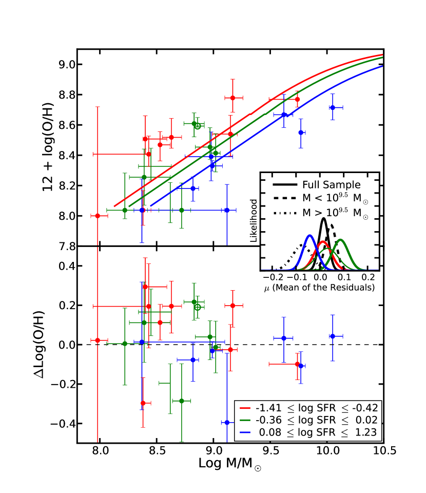
Figure 7.— The fundamental metallicity relation, derived using the Maiolino et al. (2008) metallicity calibration, shows that low mass galaxies with high SFRs have systematically lower metallicities. The galaxy 23.5+2-0.33, which strongly influences the weighted mean of the residuals (see text), is shown as an open green symbol. Top- The MZ relation is plotted, with galaxies color-coded in three bins of SFR. The curves show the local FMR reported by Mannucci et al. (2011). FMR. Bottom– Residuals from the local FMR (data minus relation given in Equation 1) show increased scatter towards low stellar masses, owing to larger measurement errors for faint galaxies. (Note that residuals are calculated using measured SFRs rather than the mean values where Equation 1 has been evaluated for the top panel. As a result the residuals in the bottom panel do not exactly correspond to the differences between the data and models in the top panel.) Inset– Likelihood functions for the mean of the residuals are shown for different subsets of the data, including the full sample, low and high mass subsamples, and the SFR divided subsamples. With one exception, the likelihood functions shown here include the galaxy 23.5+2-0.33, which drives some of the trends towards larger positive residuals (see text). The thin green curve shows the effect of removing this outlier.

Figure 7 compares our galaxies to the $z=0.1$ FMR reported in Mannucci et al. (2011). On the top panel, we show the MZ relation, with our data points color coded by three different SFR bins. The FMR, which is evaluated and shown for the same three SFR bins, is given by the relation (Equation 2 from Mannucci et al. 2011):

$$\begin{array}[]{ll}12+{\rm log(O/H)}&=8.90+0.37m-0.14s-0.19m^{2}\\ &+0.12ms-0.054s^{2}~{}~{}~{}~{}~{}~{}~{}~{}\rm{for}~{}\mu_{0.32}\geq 9.5\\ \\ &=8.93+0.51(\mu_{0.32}-10)~{}\rm{for}~{}\mu_{0.32}<9.5,\\ \end{array}$$ (1)

where $m={\rm log}(M)-10$, $s={\rm log}(\rm{SFR})$, and $\mu_{32}={\rm log}(M)-0.32{\rm log}({\rm SFR})$. This exercise shows clearly that a planar relation exists to lower masses at $z\sim 0.6-0.7$, with low SFR galaxies showing higher metallicities. To highlight the differences from the FMR, the bottom panel shows the residuals from the local plane. Here, we have included the uncertainty in the SED-derived SFR, as it enters into the metallicity that is predicted by the local FMR. Overall, we see that most galaxies have metallicities that fall within 0.2 dex of the local FMR, However, at low masses and low SFRs there are more objects with $\Delta$log (O/H) $>0$, so it is reasonable to question whether these galaxies deviate slightly from the FMR. Therefore, we calculate the mean of the residuals, $\mu=\langle\Delta$log (O/H)$\rangle$, and its uncertainty by using a maximum likelihood estimation to account for the individual measurement errors. Under this approach, the probability of observing a galaxy with a residual $y_{i}$ and error, $\sigma_{i}$ is $p_{i}=e^{-(y_{i}-\mu)^{2}/2\sigma_{i}^{2}}$. Then, for the full sample the likelihood function becomes $\mathcal{L}(\mu)=\prod p_{i}$. We evaluate this likelihood function between $-0.4<\mu<0.4$, taking the maximum and the 68% confidence intervals of $\mathcal{L}(\mu)$ to represent the mean and its error. This estimate is made for the full sample, as well as low and high mass subsamples (divided at $10^{9.5}M_{\sun}$) and the subsamples in three bins of SFR.

In the inset panel of Figure 7, we show the likelihood functions for the mean of the FMR residuals. These calculations indicate only insignificant deviations from the local FMR. In Table 4, we give the mean of the residuals and its uncertainty for the full sample and various subsamples. At first glance, we see two weakly significant deviations from the local plane: one among the lower mass ($M<10^{9.5}$ M_☉) galaxies, and the other for those with intermediate SFRs (green points). However, upon closer inspection we find that these trends arise solely because of one galaxy (23.5+2-0.33) with a metallicity 3.4$\sigma$ above the fundamental plane. (Furthermore, this galaxy has a strong influence on our calculation not because its residual is large, but rather because its errors are small.) Without this galaxy, the deviation disappears (see the thin green curve in the inset of Figure 7), and the mean of the residuals fall within 1.5$\sigma$ of zero for all of the subsamples listed in Table 4. Since any claims of a deviation from the FMR should be based on more than one object, we conclude that our data show no compelling evidence for evolution at $10^{8}<M/M_{\sun}<10^{9.5}$. This result lends greater leverage to the finding that the FMR is not evolving for higher mass galaxies at these redshifts (Cresci et al., 2012).

Table 4Residuals from the local FMR

Sample	Mean of the Residuals, $\mu$
Full sample	$0.016\pm 0.020$
$M>10^{9.5}$ M☉	$-0.074\pm 0.083$
$M<10^{9.5}$ M☉	$0.046\pm 0.022$
$-1.41\leq$ log SFR $\leq-0.42$	$0.013\pm 0.035$
$-0.36\leq$ log SFR $\leq~{}~{}0.02$	$0.086\pm 0.033$
$0.08\leq$ log SFR $\leq~{}~{}1.23$	$-0.042\pm 0.029$
Without 23.5+2-0.33
Full Sample	$-0.009\pm 0.021$
$-0.36\leq$ log SFR $\leq 0.02$	$0.027\pm 0.043$
$M<10^{9.5}$ M☉	$0.018\pm 0.025$

It is also interesting to examine the scatter about the FMR, as intrinsic scatter could indicate that there are additional physical processes that influence gas-phase metallicities. For intermediate redshift galaxies, Cresci et al. (2012) report a scatter of 0.11 to 0.14 dex about the FMR. Yet, in our sample, the scatter appears to be larger at lower masses. We find an RMS of 0.2 dex below $M<10^{9.5}$ M_☉. Assigning some galaxies to the lower branch of R23 does not reduce this scatter. The amplitude of the residuals are larger (or the about the same for a few galaxies) when the lower metallicity solutions are adopted. In order to disentangle intrinsic scatter from increased measurement errors in faint galaxies, we use a Monte Carlo simulation. First, we assume that there is no intrinsic scatter relative to the FMR. Then, focusing only on the galaxies with $M<10^{9.5}$ M_☉, we generate 10,000 mock realizations of the FMR residuals, perturbing the data in Figure 7 by their uncertainties. We calculate the RMS about the FMR for each realization, and find a mean of 0.23 dex, in good agreement with observations. This exercise implies that the amount of scatter that we observe can be entirely explained by our measurement errors. Therefore, we conclude that the intrinsic scatter about the FMR must be small. Repeating the simulation with additional intrinsic scatter shows allows us to place an upper limit on this scatter. We find that an intrinsic scatter of 0.16 dex produces an observed RMS $\leq 0.2$ dex in only 5% of Monte Carlo realizations. Remarkably, the scatter about the FMR for the present sample is significantly smaller than the 0.4 dex RMS found for similar mass galaxies in the local universe (Mannucci et al., 2011). We therefore conclude that the increased scatter in the low mass, $z=0.1$ FMR is likely the result of increased measurement uncertainties for faint galaxies.

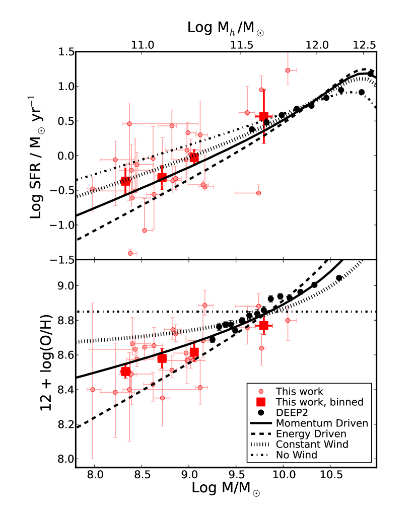
Figure 8.— The SFR-M_∗ correlation (top) and MZ relation (bottom) constrain models from Davé et al. (2012). Large red squares show the average mass, metallicity, and SFR for four mass bins: $M>10^{9.5}M_{\sun}$, $10^{8.9}<M/M_{\sun}<10^{9.2}$, $10^{8.5}<M/M_{\sun}<10^{8.9}$ and $M<10^{8.5}$ M_☉. Error bars on the binned data represent the standard deviation of the mean. We combine our data with binned higher mass data from DEEP2: the $z=0.5-0.7$ SFR - M_∗ correlation reported by Noeske et al. (2007; converted to a Chabrier 2003 IMF), and the $z\sim 0.8$ MZ relation from Zahid et al. (2011). MZ models are normalized by taking a nucleosynthetic yield that minimizes $\chi^{2}$ for the union of our data and the Zahid et al. data. SFR-M_∗ models are not renormalized. The models are described in detail in §7.1. The halo mass scale shown at the top assumes the $M_{*}-M_{halo}$ relation from Moster et al. (2010).

7. Constraining Gas Flows with the Mass-Metallicity and SFR-M_⋆ Relations

As we introduced in §1, the MZ relation is an important measure of galaxy evolution. Galaxies are not closed boxes; gas must be accreted from the IGM to fuel star formation (e.g.  Erb 2008; Bouché et al. 2010), and galactic outflows are commonly observed at both low and high-redshift (e.g.  Heckman et al. 1990; Martin 2005; Henry et al. 2007; Soto et al. 2012; Kornei et al. 2012; Erb et al. 2012). The MZ relation provides an independent, albeit indirect, constraint on these gaseous flows. On one hand, the accretion of primordial gas will reduce the gas-phase metallicity in a galaxy. On the other hand, galactic winds can create a deviation from the closed-box model by lowering the gas fraction without changing the metallicity (Edmunds, 1990; Dalcanton, 2007). Combining our data with the higher mass MZ relation provides an important increase in dynamic range that allows for more stringent constraints on models.

Our emission line selection of galaxies does not strongly bias our sample or hamper our ability to test theoretical models. In Figure 5 we show that our sample is consistent with the DEEP2 MZ relation reported by Zahid et al. (2011; at least in the limited mass range where our data overlap). This agreement can be understood, since the FMR dependence on the SFR is relatively weak. For example, if the SFRs of our galaxies were biased high by a factor of several, then (following the Mannucci et al. 2011 FMR) an “unbiased” sample would have metallicities which are approximately 0.1 dex higher. An increase in metallicity this large is implausible, as it would imply a lack of metallicity evolution inconsistent with other studies. Likewise, it is worth pointing out that the high S/N of the spectra shown in Figures 1 and 2 implies that our sample is not biased towards higher metallicities by a requirement for strong H$\beta$ emission. The objects which were excluded due to low S/N all fell among the class #3 objects discussed in §2.1; these are either extremely faint, low-mass galaxies with uncertain optical counterparts, or brighter galaxies that fell partially outside our slit. These galaxies have poorer quality spectra overall; it is unlikely that their exclusion biases our results.

In order to further verify that our sample is not biased by emission-line selection, we place our galaxies on the SFR-M_∗ relation (i.e. the star-forming main sequence) in the top panel of Figure 8. This comparison demonstrates that our galaxies do not have extreme SFRs for their stellar masses. Rather, they lie on an extrapolation of the relation reported by Noeske et al. (2007). Our sample could only be significantly biased if the “true” SFR-M_∗ relation turns over and becomes steeper at low stellar masses. While this trend is predicted to occur when photoionization heating suppresses star formation in low mass halos, it is not expected to be important above $M_{halo}\gtrsim 10^{9}M_{\sun}$ (Okamoto et al., 2008). While beyond the scope of this paper, it is worth noting that we do not detect the flattening of the SFR-M_∗ relation at low masses which is reported by Pirzkal et al. (2012).

7.1. Theoretical Framework

One set of models which have recently gained traction are those that adopt an equilibrium between mass inflow ($\dot{M}_{in}$), outflow ($\dot{M}_{out}$), and gas consumption via star formation ($\dot{M}_{*}$; Bouché et al. 2010; Dutton et al. 2010; Finlator & Davé 2008; Davé et al. 2012). These models provide a relatively simple interpretation of the FMR as a manifestation of stochastic star formation. When a galaxy accretes gas, its metallicity is diluted and its star formation increases. The increased star formation serves to consume the extra gas and return the galaxy to its equilibrium. Likewise, a pause in gas accretion will lower star formation rates and increase gas-phase metallicities until accretion resumes. These models not only predict a MZ relation, but also the SFR-M_∗ relation that we have shown in Figure 8. above. Therefore, in the remainder of this section we leverage the two relations to gain the best possible constraints on the models.

Quantitatively, we can express the equilibrium condition as (reproducing Equation 1 from Davé et al. 2012):

$$\dot{M}_{in}=\dot{M}_{out}+\dot{M}_{*}.$$ (2)

Following this assumption, Finlator & Davé (2008) and Davé et al. (2012) show that SFRs and metallicities can be written as:

$$SFR={{\zeta\dot{M}_{grav}}\over{(1+\eta)(1-\alpha_{z})}}$$ (3)

and

$$Z_{O}={{y\over{1+\eta}}{1\over{1-\alpha_{Z}}}}.$$ (4)

The quantities in Equations 3 and 4 are defined as follows:

1. $Z_{O}$ is taken to represent the mass fraction of oxygen in the ISM. This quantity is converted to the units of 12 + log(O/H) by taking log($Z_{O}$) = log(O/H) + log( ${3\over 4}\times M_{O}/M_{H}$ ). $M_{O}$ and $M_{H}$ are the atomic masses of oxygen and hydrogen.

2. $\dot{M}_{grav}$ is the cosmological baryonic accretion rate, taken from Dekel et al. (2009). Because this quantity (as well as others below) are expressed in terms of halo mass, we adopt the $M_{*}-M_{halo}$ relation from Moster et al. (2010).

3. $\zeta$ is a quantity that represents preventive (rather than ejective) feedback from gas heating. There are multiple forms of preventive feedback, and they combine multiplicatively. In the range of halo-masses where our objects lie, the most important of these is gravitational heating from virial shock formation in accreted gas. Following Davé et al. (2012), we take the analytical form given by Faucher-Giguere et al. (2011):

   $$\zeta_{grav}\approx 0.47{\left({1+z}\over 4\right)}^{0.38}{\left({M_{halo}}\over{10^{12}~{}M_{\sun}}\right)}^{-0.25}.$$ (5)

   At high masses star formation quenching associated with supermassive black holes becomes important. While we do not aim to constrain quenching, we implement it following Davé et al. (2012):

   $$\zeta_{quench}=\left(1+1/3\left({M_{halo}}\over{10^{12.3}M_{\sun}}\right)^{2}\right)^{-1.5}.$$ (6)

   The mass scale that we have adopted for $\zeta_{quench}$ is for $z=0$, and while it may be higher at earlier cosmic times (Dekel et al., 2009), the exact scaling is unimportant in the present analysis. At the low mass end, we take the photoionization feedback to be unimportant; as mentioned above, it is not expected to play a significant role at $M_{halo}\gtrsim 10^{9}M_{\sun}$. Finally, Davé et al. (2012) do note that heating by galactic winds may be important, but the physics of this effect is poorly understood. As such, they adopt an arbitrary parameterization of $\zeta_{winds}$ to consider its qualitative effects. As we will show below, this additional heating is not needed to reproduce the present data.

4. $y$ is the nucleosynthetic yield of oxygen, which is between $0.008<y<0.021$ (Finlator & Davé, 2008). Since metallicity calibrations are uncertain (Kewley & Ellison, 2008), we take $y$ as a free parameter as we search for a normalization that best matches our observed MZ relation. Hence, our comparison to the MZ relation concerns its slope, but not the normalization.

5. $\eta$ is the mass loading factor, which is defined as the ratio of the outflow rate to the SFR: $\eta=\dot{M}_{out}/\dot{M}_{*}$. In the comparison that follows, we adopt mass-loading factors that correspond (respectively) to momentum- and energy- driven winds (i.e. Murray et al. 2005; Finlator & Davé 2008; Davé et al. 2011b; Peeples & Shankar 2011; Davé et al. 2012):

   $$\eta=(M_{halo}/10^{12}M_{\sun})^{-1/3}$$ (7)

   $$\eta=(M_{halo}/10^{12}M_{\sun})^{-2/3}.$$ (8)

   The normalizations of these $\eta$ are taken from Davé et al. (2012). In addition to these two parameterizations of $\eta$, we compare to the case of no winds ($\eta=0$), also $\eta=1$, where the mass loss rate is fixed to the SFR.

6. Finally, the quantity $\alpha_{Z}$ is the ratio of the metallicities of infalling gas and the ISM: $Z_{in}/Z_{ISM}$. The inclusion of $\alpha_{Z}$ allows for enriched inflows (possibly from previously ejected material now being re-accreted from the galaxy halo). Additionally, it appears in the model for SFR as a simple way to quantify the recycling of enriched halo gas into the ISM (i.e. an additional source of fuel for star formation). The parameterization of $\alpha_{z}$ is taken from momentum-driven wind simulations in Davé et al. (2011b, 2012):

   $$\alpha_{Z}=(0.5-0.1z)(M_{*}/10^{10}M_{\sun})^{0.25}$$ (9)

   (although they note that it is a “crude” parameterization). While we aim to test models beyond those that are momentum-driven, $\alpha_{z}$ is not reported for these simulations. Therefore we use this parameterization for all of the models with winds. For the no wind case we consider $\alpha_{z}=0$, since there can be no recycling of previously ejected material in this scenario. We consider the effects of modifying $\alpha_{z}$ in the discussion below.

7.2. Comparison of equilibrium models to intermediate-redshift data

Figure 8 shows how the equilibrium models compare to the intermediate-redshift MZ and SFR-M_∗ relations. In order to get the best constraints on the models, we combine our sample with binned DEEP2 data representing the MZ relation for $z\sim 0.8$ galaxies (Zahid et al., 2011) and the SFR-M_∗ relation for $z\sim 0.5-0.7$ galaxies (Noeske et al., 2007). As we mentioned above, since metallicity calibrations and nucleosynthetic yields are uncertain, we fit for the yield that reproduces the MZ data. The yields that minimize $\chi^{2}$ (including uncertainties in both metallicity and mass) are $y=0.012,0.013,0.010$ and 0.008 for the momentum driven, energy driven, constant wind ($\eta=1$) and no wind ($\eta=0$, $\alpha_{z}=0$) models respectively. We next describe how each model compares to the data:

No wind

Not surprisingly, equilibrium models that exclude outflows are unable to reproduce the data. Most drastically, when $\eta=0$ and $\alpha_{z}=0$, Equation 4 has no mass dependence. Hence, the predicted MZ relation is implausibly flat, and the slope of SFR-M_∗ relation is also too flat. Figure 8 shows that, without winds low mass galaxies make too many stars (and metals), and are unable to get rid of the metals that they make. It is worth noting that $\alpha_{z}$ is not strictly zero in the no-wind simulation (Davé et al., 2011a), since infalling gas can be enriched by other galaxies or could represent the accretion of a satellite galaxy. A non-zero $\alpha_{z}$ would further increase the SFR and amplify the disagreement between the SFR-M_∗ data and the no-wind model.

Constant Wind

A model where the mass-loss rate is equivalent to the SFR shows good agreement with the SFR-M_∗ relation at all stellar masses. However, this model predicts an MZ relation which is too flat at low stellar masses.

Momentum Driven Wind

Of the models shown in Figure 8, the momentum driven wind shows the best match to the MZ data. However, the metallicities predicted by this model turn up at higher masses, owing to the dependence on $\alpha_{z}$. Equation 4 shows that the predicted metallicities diverge as $\alpha_{z}$ approaches unity at higher masses. While the disagreement between the model and data is only apparent in the highest mass bin, the upturn remains implausible. Locally, the MZ relation flattens to higher masses (Tremonti et al., 2004), so the model shown in Figure 8 crosses the $z\sim 0.1$ relation at $M\sim 10^{10.5}$ M_☉. This observation suggests that the mass scaling for $\alpha_{Z}$ given by Davé et al. (2012) may be too steep at high masses.

In addition to the MZ relation, we compare the momentum-driven wind model to the SFR-M_∗ relation in the top panel of Figure 8. In this case, the model slightly under-predicts the SFRs for the galaxies in the present study as well as for the lower mass DEEP2 measurements. This discrepancy between the data and models at low masses is qualitatively similar to what is found at higher masses and lower redshifts. Davé et al. (2011a) and Weinmann et al. (2012) find that both simulations and semi-analytic models are unable to reproduce the population of low mass galaxies with high specific SFRs.

Given the uncertainty in $\alpha_{z}$, we next consider whether modifying this variable can produce a momentum driven wind model that is a good fit to both the MZ and SFR-M_∗ data. If we remove the mass-dependence of $\alpha_{z}$ in Equation 9 ($\alpha_{z}\propto M_{*}^{0.0}$), the predicted SFR-M_∗ relation appears very similar to the constant wind model (a good match to the data), but the predicted MZ relation (not shown) is far too flat. In summary, modifying $\alpha_{z}$ does not improve the agreement between the data and the momentum driven wind model.

Energy Driven Wind

The energy driven wind models shown in Figure 8 are too steep compared to both the MZ data and the SFR-M_∗ data. However, as we already noted, some of this steepening of the MZ relation occurs because $\alpha_{z}$ may be too large at high masses. In fact, an energy driven wind model with $\alpha_{z}\propto M_{*}^{0.0}$ and $y=0.022$ appears very similar to the momentum driven wind model shown in both the top and bottom panels. For this model, the MZ relation model reduces to a straight line that runs through all of the data, and SFRs are slightly under-predicted at low masses. Ultimately, we cannot distinguish the momentum driven model from an energy driven model with $\alpha_{z}\propto M_{*}^{0.0}$. However, we do note that this variable shows some mass dependence in the momentum-driven wind simulations (Davé et al., 2011a, b), so it unlikely that this dependence is non-existent for energy-driven winds. We therefore conclude that energy-driven winds are unlikely to explain the data.

Recent simulations from Hopkins et al. (2012) have suggested that outflows depend strongly on gas surface density, so that winds from low density dwarf galaxies are dominated by energy-driving from supernovae and stellar winds. More massive star-forming galaxies with higher gas densities, on the other hand, are predicted to prefer momentum driven winds. The present data do not indicate a mass-dependent $\eta$; Figure 8 shows no evidence for steeper MZ and SFR-M_∗ slopes towards lower masses.

This analysis (and Figure 8) shows that there may be a tension between the data and the equilibrium model. On one hand, models which best match the MZ relation under-predict the amount of star formation in low mass galaxies (and even intermediate masses probed by DEEP2). Likewise, models that best reproduce the SFR-M_∗ relation over-predict the metallicities of galaxies. This trend can be understood as a generic property of the models, because both Equations 3 and 4 are proportional to $(1+\eta)^{-1}(1-\alpha_{z})^{-1}$; changes in these model components alter the MZ and SFR-M_∗ relation in the same manner. However, if preventive feedback from gas heating has been overestimated ($\zeta$ underestimated in Equations 3 and 5), then SFRs can be increased without modifying the MZ relation. In fact, Davé et al. (2012) note that $\zeta_{grav}$ is taken from simulations that do not include metal-line cooling (Faucher-Giguere et al., 2011), and raise the question of whether this effect is important. Alternatively, if $\zeta$ is correct, then the data may suggest a deviation from the equilibrium model.

Ultimately, we conclude that this disagreement remains subtle. While we have argued that emission line selection does not largely bias our results, we cannot rule out a small effect. As an example, if the SFRs presented in Figure 8 are high by 0.1 dex, we would expect an unbiased sample to have an SFR-$M_{*}$ relation that agrees better with the momentum driven wind model at low masses. Additionally, according to the FMR, SFRs which are 0.1 dex lower should be accompanied by metallicities which are around 0.03 dex higher, in even better agreement with the momentum driven wind MZ relation. Even without emission-line selection bias, it is important to recall that the [O II], H$\beta$, and SED-based SFR indicators discussed in the Appendix differ systematically by up to 0.2 dex. However, modifying the SFR under these scenarios can not satisfactorily bring the data in line with the momentum-driven model. Even in the higher mass data alone, this model predicts a steeper SFR-$M_{*}$ relation than the DEEP2 result (Noeske et al., 2007); therefore, the discrepancy which we have identified is apparent in a magnitude-limited sample. We conclude that H$\alpha$ followup spectroscopy of our sample (combined with a mass selected control sample) can definitively assess the effects of emission line selection, while simultaneously reducing errors on dust, SFR, and metallicity. We leave this work as the subject of a future paper.

Finally, it is worth pointing out that systematic uncertainties in our metallicity calibration cannot explain the discrepancy between the data and models. Kewley & Ellison (2008) show that local (SDSS) MZ relations have similar low mass slopes under most calibrations. The Tremonti et al. (2004) calibration and the direct-method electron temperature calibration (Andrews & Martini, 2013) are two exceptions– both produce MZ relations that are steeper than what we have used here. Hence, if we calculated metallicities in the same way as Tremonti et al. or by using electron temperatures, the tension between the data and models would be amplified. On the other hand, the calibrations reported by Pilyugin (2001) and Pilyugin & Thuan (2005) give MZ relations that are flatter than most. However, we note that they also have metallicities around 0.5-0.7 dex lower than those from KK04. These lower metallicities would introduce other difficulties, as they would require normalizing yields that fall below the plausible range indicated in Finlator & Davé (2008).

8. Conclusions

In this work we have placed the first constraints on the low mass, intermediate redshift MZ relation. By using emission line selection in the COSMOS field, we are able to efficiently identify and measure the metallicities from 26 galaxies reaching masses of $10^{8}$ M_☉ at $z\sim 0.65$. Combined with previous measurements from magnitude limited samples, these data extend our knowledge of the MZ relation to masses an order of magnitude smaller. This limit is comparable to the low mass limit of the local MZ relation determined from SDSS data. Therefore, for the first time we are able to measure the metallicity evolution of intermediate redshift galaxies at $M<10^{9}$ M_☉. Compared to the $z\sim 0.1$ relation reported by Tremonti et al. (2004), we find an average metallicity that is 0.12 dex lower for galaxies with $10^{8.5}<M/M_{\sun}<10^{9.0}.$ We show that this measurement is consistent with an MZ relation that evolves more strongly at low stellar masses. We interpret this mass-dependent evolution as consistent with downsizing trends, where higher mass objects have less leverage to alter their gas-phase metallicities after most of their stars have been assembled.

An important development in our understanding of metallicity evolution is the discovery that the scatter in the relation can be reduced by accounting for star formation. This measurement was quantified as a plane, and dubbed the Fundamental Metallicity Relation (FMR) by Mannucci et al. (2010). Using the present sample, we find that a planar relation does indeed exist among low mass, intermediate redshift galaxies. Consistent with the findings of Mannucci et al., we see no evidence for evolution of the FMR, as our emission-line selected sample falls in good agreement with their $z\sim 0.1$ FMR (Mannucci et al., 2011). Furthermore, while the lowest mass galaxies in our sample show significant scatter with respect to the FMR, we attribute this scatter to measurement uncertainties for faint galaxies. Using a Monte Carlo simulation, we determine that the intrinsic scatter is consistent with zero, and should be less than 0.16 dex (95% confidence) at $M<10^{9.5}$ M_☉.

The MZ relation is an important probe of galaxy evolution models, as accretion and galactic outflows modulate the gas-phase metallicities of galaxies. Hence, comparison to model predictions can help us to gain insight into galaxy formation. We have combined our MZ relation with the SFR-M_∗ correlation that is also measured from our data, taking higher mass data from the literature (Noeske et al., 2007; Zahid et al., 2011). We compare to the family of models outlined in Davé et al. (2012), where it is assumed that galaxies prefer to maintain an equilibrium between inflows, outflows, and star formation (Finlator & Davé, 2008; Bouché et al., 2010; Dutton et al., 2010; Davé et al., 2012). We find that models which predict the MZ relation may under-predict the SFRs of low mass galaxies, and at the same time, models that predict the SFRs of low mass galaxies tend to over-predict their metallicities. While this finding could represent a breakdown of the equilibrium model in low mass galaxies, it could alternatively be an indication that feedback from gas-heating has been overestimated in simulations (i.e. Faucher-Giguere et al. 2011). To solidify this result, we have begun H$\alpha$ and [N II]  spectroscopy to followup the present sample and simultaneously measure a mass-selected control sample. These data will clarify the effects of emission line selection and greatly reduce the statistical uncertainties in our metallicity, dust, and SFR measurements.

To conclude, these observations have provided a valuable look at the metallicity evolution of low mass galaxies outside the local universe. We look forward to the physical insights and new constraints that can be gained from larger samples and a better characterization of systematic uncertainties.

Appendix A Assessing SFR measurements

In §6 and §7 we draw conclusions from SFRs that we derived from SED fits; therefore, it is important that we use reliable SFRs. In order to assess systematic uncertainties, we compare this measurement to two additional SFR indicators: H$\beta$ and [O II]. For the H$\beta$ method, we use the dust extinction from the SED fits, scaled up by a factor of 2.3 to account for the difference between stellar and nebular extinction (Calzetti et al., 2000). We also correct the H$\beta$ fluxes for the small amount of stellar absorption, as discussed above. Next, the H$\beta$ luminosities are converted to H$\alpha$, assuming a Balmer decrement of 2.8. We then use the H$\alpha$-SFR calibration given by Kennicutt (1998), scaled appropriately to a Chabrier (2003) IMF. To derive SFRs from [O II] luminosity, we use the calibration given by Moustakas et al. (2006), which includes an $M_{B}$ dependence, but does not require that the line measurement be corrected for dust.

In order to make a direct comparison to the SED-derived SFRs, we must correct the emission line fluxes for both slit losses and and extraction aperture losses. Rather than model these losses (which would not account for uncertainties in the absolute flux calibration), we compare our data to narrowband imaging in COSMOS. First, we infer the emission line flux from the narrowband (NB816) photometry, using the methods outlined in Ly et al. (2007) and Takahashi et al. (2007). Since the NB816 bandpass has a non-uniform throughput, we calculate a correction to this flux based on the relative throughput at the observed wavelengths of the emission lines. (This correction can be important, since it is not unusual that both of the [O III] doublet lines are found away from the central wavelength of the NB816 filter.) Because the COSMOS catalog contains total magnitudes (under the reasonable assumption that the galaxies are unresolved with 1.5″ FWHM spatial resolution), the line fluxes inferred from narrowband imaging are not subject to aperture losses. For 17 galaxies in our sample with emission lines that are bright enough to be detected in the narrowband imaging, we can infer the aperture losses by comparing these narrowband imaging fluxes to our spectroscopic fluxes. We find typical correction factors of 1.1-2.0, with a median of 1.4. We adopt this average correction to explore systematic differences between star formation indicators.

Figure 9 compares the SFRs derived from the SEDs, H$\beta$, and [O II]. In addition to the SED fits described in §3.2 (which use exponentially declining star formation histories with $\tau$ as a free parameter; red points), we also make the comparison for constant star-forming models (blue points). This exercise shows that the SFRs derived using different methods are correlated, so that we can easily distinguish the galaxies with high and low SFRs. However, Figure 9 also shows that there are systematic shifts as large as 0.2 dex between the different estimators. Determining the most accurate star formation indicator is beyond the scope of this paper. Ultimately, a systematic uncertainty of 0.2 dex does not affect our conclusions. In §6, we show that the scatter in the MZ relation is correlated with SFRs. As with the local FMR, metallicity depends only weakly on the SFR, so that a 0.2 dex offset in SFR translates to a 0.03 dex shift in the metallicity predicted by the local FMR (Mannucci et al., 2010, 2011). This difference in metallicity is much smaller than the uncertainties on the FMR residuals shown in Figure 7. Likewise, in §7 we use our SFR-M_∗ relation to constrain models. However, 0.2 dex of systematic uncertainty is small compared to the dynamic range of SFRs shown in Figure 8. An systematic offset is unlikely to alter our conclusions, as the SFR-M_∗ trends discussed in §7 can be seen (albeit less obviously) from the higher mass data alone.

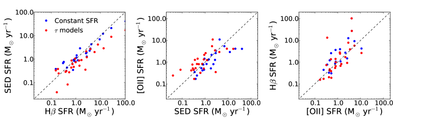
Figure 9.— Star formation rates derived three different methods are compared. Blue points assume a constant star formation history, and the red points assume exponentially declining SFRs ($\tau$ models) discussed in §3.2 The H$\beta$-derived SFRs are corrected for dust extinction using these SED fits. (The center and right panels– where the SED-independent [O II] SFRs are compared– show that the $\tau$ models tend towards slightly less dust.) The [O II] and H$\beta$ SFRs are corrected by an average factor of 1.4 to account for slit-losses. Systematic shifts between the different indicators are at most 0.2 dex.

References

- Allende Prieto et al. (2001) Allende Prieto, C., Lambert, D. L., & Asplund, M. 2001, ApJ, 557, L63
- Andrews & Martini (2013) Andrews, B. H., & Martini, P. 2013, ApJ, 765, 140
- Atek et al. (2011) Atek, H., Siana, B., Scarlata, C., et al. 2011, ApJ, 743, 121
- Baldwin, Phillips, & Terlevich (1981) Baldwin, J. A., Phillips, M. M., & Terlevich, R. 1981, PASP, 93, 5
- Berg et al. (2012) Berg, D. A., Skillman, E. D., Marble, A. R., et al. 2012, ApJ, 754, 98
- Bouché et al. (2010) Bouche, N., Dekel, A., & Genzel, R., et al. 2010, ApJ, 718, 1001
- Brinchmann et al. (2004) Brinchmann, J., Charlot, S., White, S. D. M., et al. 2004, MNRAS, 351, 1151
- Brinchmann et al. (2008) Brinchmann, J., Pettini, M., & Charlot, S. 2008, MNRAS, 385, 769
- Brooks et al. (2007) Brooks, A., Governato, F., Booth, C. M., et al. 2007, ApJ, 655, 17L
- Bruzual & Charlot (2003) Bruzual, G. & Charlot, S. 2003, MNRAS, 344, 1000
- Bruzual (2007) Bruzual, G. 2007, ASPC, 374, 303
- Calzetti et al. (2000) Calzetti, D., Armus, L., Bohlin, R. C., et al. 2000, ApJ, 533, 682
- Capak et al. (2007) Capak, P., Aussel, H., Ajiki, M., et al. 2007, ApJS, 172, 99
- Cardelli et al. (1989) Cardelli, J. A., Clayton, G. C., & Mathis, J. S. 1989, ApJ, 345, 245
- Chabrier (2003) Chabrier, G. 2003, PASP, 115, 763
- Conroy & Gunn (2010) Conroy, C., & Gunn, J. E. 2010, ApJ, 172, 833
- Cooper et al. (2012) Cooper, M. C., Newman, J. A., Davis, M., Finkbeiner, D. P., Gerke, B. F. 2012, ASCL, 1203.003
- Cowie & Barger (2008) Cowie, L. L., & Barger, A. J. 2008, ApJ, 686, 72
- Cresci et al. (2010) Cresci, G., Mannucci, F., Maiolino, R., et al. 2010, Nature, 467, 811
- Cresci et al. (2012) Cresci, G., Mannucci, F., Sommariva, V., et al. 2012, MNRAS, 421, 262
- Dalcanton (2007) Dalcanton, J. J. 2007, ApJ, 658, 941
- Davé et al. (2011a) Davé, R., Oppenheimer, B. D., & Finlator, K.,2011, MNRAS, 415, 11
- Davé et al. (2011b) Davé, R., Finlator, K., & Oppenheimer, B. D. 2011, MNRAS, 416, 1354
- Davé et al. (2012) Davé, R., Finlator, K., & Oppenheimer, B. D., 2012, MNRAS, 421, 98
- Dayal et al. (2013) Dayal, P., Ferrara, A., & Dunlop, J. S. 2013, MNRAS, 430, 2891
- Dekel et al. (2009) Dekel, A., Birnboin, Y., Engel, G., et al. 2009, Nature, 457, 451
- Dressler et al. (2011a) Dressler, A., Martin, C. L., Henry, A., Sawicki, M., & McCarthy, P. 2011, ApJ, 740, 71
- Dressler et al. (2011b) Dressler, A., Bigelow, B., Hare, T., et al. 2011, PASP, 123, 288
- Dutton et al. (2010) Dutton, A. A., van den Bosch, F. C., Dekel, A. 2010, MNRAS, 405, 1690
- Edmunds (1990) Edmunds, M. G. 1990, MNRAS, 246, 678
- Elbaz et al. (2007) Elbaz, D., Daddi, E., Le Borgne, D., et al. 2007, A&A, 468, 33
- Ellison et al. (2008) Ellison, S., Patton, D. R., Simard, L., & McConnachie, A. W. 2008, ApJ, 672, 107L
- Erb et al. (2006) Erb, D. K., Shapley, A. E., Pettini, M., et al. 2006, ApJ, 644, 813
- Erb (2008) Erb, D. K. 2008, ApJ, 674, 151
- Erb et al. (2012) Erb, D. K., Quider, A. M., Henry, A. L., & Martin, C. 2012, ApJ, 759, 26
- Faber et al. (2003) Faber, S. M., Phillips, A. C., Kibrick, R.I., et al. 2003, SPIE, 4841, 1657
- Faucher-Giguere et al. (2011) Faucher-Giguere, C. A., Keres, D., & Ma, C.-P. 2011, MNRAS, 417, 2982
- Fillipenko (1982) Fillipenko, A. V. 1982, PASP, 94, 715
- Finlator & Davé (2008) Finlator, K., & Davé, R. 2008, MNRAS, 385, 2181
- Finlator et al. (2011) Finlator, K., Oppenheimer, B. D., Davé, R. 2011, MNRAS, 410, 1730
- Hainline et al. (2009) Hainline, K. N., Shapley, A. E., Kornei, K. A., et al. 2009, ApJ, 701, 52
- Heckman et al. (1990) Heckman, T. M., Armus, L., & Miley, G. K. 1990, ApJS, 74, 833
- Henry et al. (2012) Henry, A. L., Martin, C. L., Dressler, A., Sawicki, M., & McCarthy, P. 2012, ApJ, 744, 149
- Henry et al. (2007) Henry, A. L., Turner, J. L., Beck, S. C., Crosthwaite, L. P., & Meier, D. S. 2007, AJ, 133, 757
- Hopkins et al. (2012) Hopkins, P. F., Quataert, E., & Murray, N. 2012, MNRAS, 421, 3522
- Hu et al. (2009) Hu, E., Cowie, L. L., Kakazu, Y. & Barger, A. 2009, ApJ, 698, 2014
- Ilbert et al. (2009) Ilbert, O., Capak, P., Salvato, M., et al. 2009, ApJ, 690, 1236
- Juneau et al. (2011) Juneau, S., Dickinson, M., Alexander, D. M., & Salim, S. 2011, ApJ, 736, 104
- Kakazu et al. (2007) Kakazu, Y., Cowie, L. L., & Hu, E. M. 2007, ApJ, 668, 853
- Kashikawa et al. (2011) Kashikawa, N., Shimasaku, K., Matsuda, Y., et al. 2011, ApJ, 648, 7
- Kewley & Dopita (2002) Kewley, L. J., & Dopita, M. A. 2002, ApJS, 142, 35
- Kewley & Ellison (2008) Kewley, L. J., & Ellison, S. L. 2008, ApJ, 681, 1183
- Kennicutt (1998) Kennicutt, R. C., 1998, ARA&A, 36, 189
- Kirby et al. (2011) Kirby, E. N., Martin, C. L., & Finlator, K. 2011, ApJ, 742, 25L
- Kniazev et al. (2003) Kniazev, A. Y., Grebel, E. K., Hao, L., et al. 2003, ApJ, 593, 73L
- Kobulnicky & Kewley (2004) Kobulnicky, H. A., & Kewley, L. J. 2004, ApJ, 617, 240
- Kornei et al. (2012) Kornei, K. A., Shapley, A. E., Martin, C. L., et al. 2012, ApJ, 758, 135
- Kriek et al. (2009) Kriek, M., van Dokkum, P. G., Labbé, I., et al. 2009, ApJ, 700, 221
- Kriek et al. (2010) Kriek, M., Labbé, I., Conroy, C., et al. 2010, ApJ, 722, L64
- Kroupa (2001) Kroupa, P. 2001, MNRAS, 322, 231
- Lamareille et al. (2009) Lamareille, F., Brinchmann, J., Contini, T., et al. 2009, A&A, 495, 53
- Lara-Lopez et al. (2010) Lara-López, M. A., Cepa, J., Bongiovanni, A., et al. 2010, A&A, 521, 53L
- Lee et al. (2006) Lee, H., Skillman, E. D., Cannon, J. M., et al. 2006, ApJ, 647, 970
- Le Fèvre et al. (2004) Le Fèvre, O., Vettolani, G., Paltani, S., et al. 2004, A&A, 428, 1043
- Liang et al. (2007) Liang, Y. C., Hammer, F., & Yin, S. Y. 2007, A&A, 474, 807
- Lilly et al. (2003) Lilly, S. J., Carollo, C. M., & Stockton, A. N. 2003, ApJ, 597, 730
- Lilly et al. (2007) Lilly, S. J., Le Fèvre, O., Renzini, A., et al. 2007, ApJS, 172, 70
- Lilly et al. (2013) Lilly, S. J., Carollo, M. C., Pipino, A., Renzini, A., & Peng, Y. 2013, arXiv:1303.5059
- López-Sánchez et al. (2012) López-Sánchez, Á. R. , Dopita, M. A., Kewley, L. J., et al. 2012, MNRAS, 426, 2630
- Ly et al. (2007) Ly, C., Malkan, M. A., Kashikawa, N., et al. 2007, ApJ, 657, 738
- Maiolino et al. (2008) Maiolino, R., et al. 2008, A&A, 488, 463
- Mannucci et al. (2010) Mannucci, F., Cresci, G., Maiolino, R., Marconi, A., & Gnerucci, A. 2010, MNRAS, 408, 2115
- Mannucci et al. (2011) Mannucci, F., Salvaterra, R., & Campisi, M. A. 2011, MNRAS, 414, 1263
- Maraston (2005) Maraston, C. 2005, MNRAS, 362, 799
- Martin et al. (2008) Martin, C. L., Sawicki, M., Dressler, A., & McCarthy, P. 2008, ApJ, 679, 942
- Martin (2005) Martin, C. L. 2005, ApJ, 621, 227
- Massey & Gronwall (1990) Massey, P., & Gronwall, C. 1990, ApJ, 358, 344
- McGaugh (1991) McGaugh, S. 1991, ApJ, 380, 140
- Moster et al. (2010) Moster, B. P., Somerville, R. S., Maulbetsch, C., et al. L. 2010, ApJ, 710, 903
- Moustakas et al. (2006) Moustakas, J., Kennicutt, R. C., & Tremonti, C. A. 2006, ApJ, 642, 775
- Moustakas et al. (2011) Moustakas, J., Zaritsky, D., Brown, M., et al. 2011, arXiv:1112.3300
- Murray et al. (2005) Murray, N., Quatert, E., & Thompson, T. A. 2005, ApJ, 618, 569
- Nagao et al. (2006) Nagao, T., Maiolino, R., & Marconi, A., 2006, A&A, 459, 85
- Newman et al. (2012) Newman, J. A., Cooper, M. C., Davis, M., et al. 2012, arXiv:1203.3192
- Nicholls et al. (2012) Nicholls, D., Dopita, M. A., & Sutherland, R. S., ApJ, 2012, 752, 148
- Noeske et al. (2007) Noeske, K. G., Faber, S. M., Weiner, B. J., et al. 2007, ApJ, 660, L47
- Okamoto et al. (2008) Okamoto, T., Gao, L., Theuns, T. 2008, MNRAS, 390, 920
- Oke (1990) Oke, J. B. 1990, AJ, 99, 1621
- Oppenheimer et al. (2009) Oppenheimer, B. D., Davé, R., & Finlator, K. 2009, MNRAS, 396, 729
- Pagel et al. (1979) Pagel, B. E. J., Edmunds, M. G., Blackwell, D. E., Chun, M. S., & Smith, G. 1979, MNRAS, 189, 95
- Peeples et al. (2009) Peeples, M. S., Pogge, R. W., & Stanek, K. Z. 2009, ApJ, 695, 259
- Peeples & Shankar (2011) Peeples, M. S., & Shankar, F. 2011, MNRAS, 417, 2962
- Peimbert & Costero (1969) Peimbert, M., & Costero, R. 1969, Bol. Obs. Ton. y Tac., 5, 3
- Pettini & Pagel (2004) Pettini, M., & Pagel, B. E. J. 2004, MNRAS, 384, 59L
- Pilyugin (2001) Pilyugin, L. S. 2001, A&A, 374, 412
- Pilyugin & Thuan (2005) Pilyugin, L. S., & Thuan, T. X. 2005, ApJ, 631, 231
- Pirzkal et al. (2012) Pirzkal, N., Rothberg, B., Ly, C., et al. 2012, ApJ, arXiv:1208.5535
- Savaglio et al. (2005) Savaglio, S., Glazebrook, K., Le Borgne, D., et al. 2005, ApJ, 635, 260
- Schaerer & de Barros (2009) Schaerer, D., & de Barros, S. 2009, A&A, 502, 423
- Shapley et al. (2005) Shapley, A. E., Coil, A. L., Ma, C.-P., Bundy, K. 2005, ApJ, 635, 1006
- Soto et al. (2012) Soto, K. T., Martin, C. L., Prescott, M. K. M., & Armus, L. 2012, ApJ, 757, 86
- Stasińska (2005) Stasińska, G. 2005, A&A, 434, 507
- Takahashi et al. (2007) Takahashi, M. I., Shioya, Y., Taniguchi, Y., et al. 2007, ApJS, 172, 456
- Tremonti et al. (2004) Tremonti, C. A., Heckman, T. M., Kauffman, G., et al. 2004, ApJ, 613, 898
- van den Bergh (1962) van den Bergh, S. 1962, AJ, 67, 486
- van Zee et al. (2006) van Zee, L., Skillman, E. D., & Haynes, M. P. 2006, ApJ, 637, 269
- Weinmann et al. (2012) Weinmann, S. M., Pasquali, A., Oppenheimer, B. D., et al. 2012, MNRAS, 426, 2797
- Wofford et al. (2013) Wofford, A., Leitherer, C., & Salzer, J. 2013, ApJ, 765, 118
- Wuyts et al. (2012) Wuyts, E., Rigby, J. R., Sharon, K., & Gladders, M. D. 2012, ApJ, 755, 73
- Xia et al. (2012) Xia, L., Malhotra, S., Rhoads, J., et al. 2012, AJ, 144, 28
- Yates et al. (2012) Yates, R. M., Kauffman, G., & Guo, Q. 2012, MNRAS, 422, 215
- Zahid et al. (2011) Zahid, H. J., Kewley, L. J., & Bresolin, F. 2011, ApJ, 730, 137
- Zhao et al. (2010) Zhao, Y., Gao, Y., & Gu, Q. 2010, ApJ, 710, 663
- Zibetti et al. (2013) Zibetti, S. Gallazzi, A., Charlot, S. Pierini, D., & Pasquali, A. 2013, MNRAS, 428, 1479