A Coarse-Grained Model for Predicting RNA Folding Thermodynamics

Abstract

We present a thermodynamically robust coarse-grained model to simulate folding of RNA in monovalent salt solutions. The model includes stacking, hydrogen bond and electrostatic interactions as fundamental components in describing the stability of RNA structures. The stacking interactions are parametrized using a set of nucleotide-specific parameters, which were calibrated against the thermodynamic measurements for single-base stacks and base-pair stacks. All hydrogen bonds are assumed to have the same strength, regardless of their context in the RNA structure. The ionic buffer is modeled implicitly, using the concept of counterion condensation and the Debye-Hückel theory. The three adjustable parameters in the model were determined by fitting the experimental data for two RNA hairpins and a pseudoknot. A single set of parameters provides good agreement with thermodynamic data for the three RNA molecules over a wide range of temperatures and salt concentrations. In the process of calibrating the model, we establish the extent of counterion condensation onto the single-stranded RNA backbone. The reduced backbone charge is independent of the ionic strength and is 60% of the RNA bare charge at 37 ^∘C. Our model can be used to predict the folding thermodynamics for any RNA molecule in the presence of monovalent ions.

Tel.: 301-405-4803

Fax: 301-314-9404

Keywords: Hairpin, pseudoknot, melting temperature, ionic buffer

1 Introduction

Since the landmark discovery that RNA molecules can act as enzymes, ¹ an increasing repertoire of cellular functions has been associated with RNA, raising the need to understand how these complex molecules fold into elaborate tertiary structures. In response to this challenge, great strides have been made in describing RNA folding^{2, 3, 4, 5}. Single molecule and ensemble experiments using a variety of biophysical methods, combined with theoretical techniques, have led to a conceptual framework for interpreting the thermodynamics and kinetics of RNA folding ^{6, 7, 8, 9, 10}. Despite these advances, there are very few reliable structural models with the ability to quantitatively predict the thermodynamic properties of RNA (see, however, refs. 11–17). The development of simple and accurate models is complicated by the interplay of several energy and length scales, which arise from stacking, hydrogen bond and electrostatic interactions. Although multiple interactions contribute to the stability of RNA, the most vexing of these are the electrostatic interactions, since the negatively charged phosphate groups make RNA a strongly charged polyelectrolyte. ¹⁸ Because of the strong intramolecular Coulomb repulsion, the magnitude of the charge on the phosphate groups has to be reduced in order for RNA molecules to fold. The softening of repulsion between the phosphate groups requires the presence of counterions. A number of factors such as the Debye length, the Bjerrum length, the number of nucleotides in RNA, as well as the size, valence and shape of counterions ¹⁹ modulate electrostatic interactions, which further complicates the prediction of RNA folding thermodynamics.

In principle, all-atom simulations of RNA in water provide a straightforward route to computing RNA folding thermodynamics. However, uncertainties in nucleic acid force fields and the difficulty in obtaining adequate conformational sampling have prevented routine use of all-atom simulations to study the folding of even small RNA molecules. At the same time, the success of using polyelectrolyte theories¹⁸ and simulations²⁰ in capturing many salient features of RNA folding justifies the development of coarse-grained (CG) models. None of the existing CG models of RNA, which have been remarkably successful in a variety of applications, ^{21, 22, 23, 24, 25} have been used to reproduce folding thermodynamics over a wide range of ion concentrations and temperature. In this paper, we introduce a force field based on a CG model in which each nucleotide is represented by three interactions sites (TIS) — a phosphate, a sugar and a base¹². The TIS force field includes stacking, hydrogen bond and electrostatic interactions that are known to contribute significantly to the stability of RNA structures. We obtain the thermodynamic parameters for the stacking and hydrogen bond interactions by matching the simulation and experimental melting data for various nucleotide dimers and for the pseudoknot from mouse mammary tumor virus (MMTV PK in Figure SS). Our description of the electrostatic interactions in RNA relies on the concept of counterion condensation, which posits that counterions condense onto the sugar-phosphate backbone and partially reduce the charge on each phosphate group. Our simulations provide a way to determine the magnitude of the reduced backbone charge by fitting the experimental data for the ion-dependent stability of RNA hairpins (L8 and L10 in Figure SS). Remarkably, experimental data on folding thermodynamics of the MMTV PK, L8, and L10 are reproduced well over a wide range of temperatures and concentrations of monovalent salt using a single set of force field parameters. Our CG force field is transferable, and hence can be adopted for other RNA molecules as well.

2 Methods

2.1 Three Interaction Site (TIS) Representation of RNA

In the TIS model, each nucleotide is replaced by three spherical beads P, S and B, representing a phosphate, a sugar and a base (Figure STACK). The coarse-grained beads are at the center of mass of the chemical groups. The energy function in the TIS model, $U_{\rm TIS}$, has the following six components,

$$U_{\rm TIS}=U_{\rm BL}+U_{\rm BA}+U_{\rm EV}+U_{\rm ST}+U_{\rm HB}+U_{\rm EL},$$ (1)

which correspond to bond length and angle constraints, excluded volume repulsions, single strand base stacking, inter-strand hydrogen bonding and electrostatic interactions. We constrain bond lengths, $\rho$, and angles, $\alpha$, by harmonic potentials, $U_{\rm BL}(\rho)=k_{\rho}(\rho-\rho_{0})^{2}$ and $U_{\rm BA}(\alpha)=k_{\alpha}(\alpha-\alpha_{0})^{2}$, where the equilibrium values $\rho_{0}$ and $\alpha_{0}$ are obtained by coarse-graining an ideal A-form RNA helix²⁶. The values of $k_{\rho}$, in units of kcal mol^-1Å^-2, are: 64 for an S$\rightarrow$P bond, 23 for an P$\rightarrow$S bond (“$\rightarrow$” indicates the downstream direction) and 10 for an S$-$B bond. The values of $k_{\alpha}$ are 5 kcal mol^-1rad^-2 if the angle involves a base, and 20 kcal mol^-1rad^-2 otherwise.

Excluded volume between the interacting sites is modeled by a Weeks-Chandler-Andersen (WCA) potential,

$$U_{\rm EV}(r) = \varepsilon_{0}\left[\left(\frac{D_{0}}{r}\right)^{12}-2\left(\frac{D_{0}}{r}\right)^{6}+1\right],\ r\leq D_{0},$$

$$U_{\rm EV}(r) = 0,\ r>D_{0},$$ (2)

which has been commonly used to study excluded volume effects in fluids. ²⁷ The precise form of $U_{\rm EV}(r)$ will not affect the results as long as $U_{\rm EV}(r)$ is short-ranged. The WCA potential is computationally efficient because it vanishes exactly beyond the contact distance $D_{0}$. To allow close approach between two bases that stack flat one on top of another, we assume $D_{0}=3.2$ Å and $\varepsilon_{0}=1$ kcal/mol for the interacting sites representing bases. With the exception of stacked bases, this choice of parameters underestimates the distance of closest approach between coarse-grained RNA groups. However, to keep the parameterization of the model as simple as possible, we use the same $D_{0}$ and $\varepsilon$ for all interacting sites. We note that the specific choice of parameters in Eq. (POT2) has little effect on the results obtained. In our simulations, stable folds are sustained by stacking and hydrogen bond interactions, $U_{\rm ST}$ and $U_{\rm HB}$, which are parameterized using experimental thermodynamic data and accurate approach distances between various RNA groups (see below).

2.2 Stacking Interactions

Single strand stacking interactions, $U_{\rm ST}$, are applied to any two consecutive nucleotides along the chain,

$$U_{\rm ST}=\frac{U_{\rm ST}^{0}}{1+k_{r}(r-r_{0})^{2}+k_{\phi}(\phi_{1}-\phi_{1,0})^{2}+k_{\phi}(\phi_{2}-\phi_{2,0})^{2}},$$ (3)

where $r$, $\phi_{1}$ and $\phi_{2}$ are defined in Figure STACK. Sixteen distinct nucleotide dimers are modeled with different $r_{0}$, $\phi_{1,0}$, $\phi_{2,0}$ and $U_{\rm ST}^{0}$. The structural parameters $r_{0}$, $\phi_{1,0}$ and $\phi_{2,0}$ are obtained by coarse-graining an A-form RNA helix. ²⁶ To estimate standard deviations of $r$ and $\phi_{1}$, $\phi_{2}$ from the corresponding values in a A-form helix, we used double helices in the NMR structure of the pseudoknot from human telomerase RNA ²⁸ (PDB code 2K96). We chose this pseudoknot because it has two fairly long stems containing six and nine Watson-Crick base pairs. We had previously conducted simulations of the two stems at $15\ ^{\circ}$C in the limit of high ionic strength ²⁵ and found that, for $k_{r}=1.4$ Å^-2 and $k_{\phi}=4$ rad^-2, the time averages of $(r-r_{0})^{2}$, $(\phi_{1}-\phi_{1,0})^{2}$ and $(\phi_{2}-\phi_{2,0})^{2}$ agreed well with the standard deviations computed from the NMR structure. The time averages were not very sensitive to a specific choice of $U_{\rm ST}^{0}$. Using $k_{r}=1.4$ Å^-2 and $k_{\phi}=4$ rad^-2, we derive $U_{\rm ST}^{0}$ from available thermodynamic measurements of single-stranded and double-stranded RNA, ^{29, 30, 31} as described below.

2.2.1 Thermodynamic parameters of dimers from experiments

In the nearest neighbor model of RNA duplexes, the total stability of a duplex is given by a sum of successive contributions $\Delta G{x-y\choose w-z}$, where $x-y$ denotes a base pair stacked over the preceding base pair $w-z$. The enthalpy, $\Delta H$, and entropy, $\Delta S$, components of $\Delta G{x-y\choose w-z}$ are known experimentally at 1 M salt concentration²⁹. Here, we make the following assumptions:

$$\Delta H{x-y\choose w-z} = \Delta H{x\choose w}+\Delta H{z\choose y}+0.5\Delta H(w-z)+0.5\Delta H(x-y),$$

$$\Delta S{x-y\choose w-z} = \Delta S{x\choose w}+\Delta S{z\choose y},$$ (4)

where $\Delta H{x\choose w}$ and $\Delta S{x\choose w}$ are the thermodynamic parameters associated with stacking of $x$ over $w$ along $5^{\prime}\rightarrow 3^{\prime}$ in one strand. Additional enthalpy gain $\Delta H(w-z)$ arises from hydrogen bonding between $w$ and $z$ in complementary strands. Our goal is to solve Eqs. (dG2) for $\Delta H{x\choose w}$, $\Delta S{x\choose w}$ and $\Delta H(w-z)$. Since the number of unknowns exceeds the number of equations, we have to make some additional assumptions.

We average the thermodynamic parameters on the left-hand side of Eqs. (dG2) for stacks ${{\rm U-A}\choose{\rm A-U}}$ and ${{\rm A-U}\choose{\rm U-A}}$, ${{\rm A-U}\choose{\rm C-G}}$ and ${{\rm U-A}\choose{\rm G-C}}$, and ${{\rm U-A}\choose{\rm C-G}}$ and ${{\rm A-U}\choose{\rm G-C}}$, because these values are similar within experimental uncertainty.²⁹ This allows us to assign $\Delta H{x\choose w}=\Delta H{w\choose x}$ and $\Delta S{x\choose w}=\Delta S{w\choose x}$ on the right-hand side of Eqs. (dG2) for all dimers, except for ${{\rm C}\choose{\rm G}}$ and ${{\rm G}\choose{\rm C}}$. Additional simplifications result from the analysis of experimental data on stacking of nucleotide dimers.^{30, 32} Experiments indicate that dimers ${{\rm A}\choose{\rm A}}$, ${{\rm U}\choose{\rm A}}$ and ${{\rm C}\choose{\rm A}}$ have similar stacking propensities and can therefore be described by one set of thermodynamic parameters. The same holds for ${{\rm C}\choose{\rm C}}$ and ${{\rm U}\choose{\rm C}}$.

The melting temperature of dimer ${{\rm A}\choose{\rm A}}$ is known from experiment, $T_{\rm m}=26$ ^∘C ³⁰. According to the assumptions above, dimer ${{\rm U}\choose{\rm A}}$ has the same melting temperature. Combining Eqs. (dG2) for ${{\rm U-A}\choose{\rm A-U}}$ and the relationship $\Delta H{{\rm U}\choose{\rm A}}=k_{\rm B}T_{\rm m}\Delta S{{\rm U}\choose{\rm A}}$, where $T_{\rm m}=299$ K and $k_{\rm B}$ is the Boltzmann constant, we can solve for $\Delta H{{\rm U}\choose{\rm A}}$, $\Delta S{{\rm U}\choose{\rm A}}$ and $\Delta H({\rm A}-{\rm U})$. By assigning $\Delta H{{\rm A}\choose{\rm A}}=\Delta H{{\rm U}\choose{\rm A}}$ and $\Delta S{{\rm A}\choose{\rm A}}=\Delta S{{\rm U}\choose{\rm A}}$ in Eqs. (dG2) for ${{\rm A-U}\choose{\rm A-U}}$, we solve for $\Delta H{{\rm U}\choose{\rm U}}$ and $\Delta S{{\rm U}\choose{\rm U}}$. Finally, we assume

$$\Delta H{{\rm U}\choose{\rm C}}=k\Delta H{{\rm U}\choose{\rm A}}+(1-k)\Delta H{{\rm U}\choose{\rm U}},$$

$$\Delta S{{\rm U}\choose{\rm C}}=k\Delta S{{\rm U}\choose{\rm A}}+(1-k)\Delta S{{\rm U}\choose{\rm U}},$$ (5)

where $k$ is a constant. This assumption is based on the observation that the measured enthalpy changes of duplex formation, $\Delta H{x-y\choose w-z}$ in Eqs. (dG2), are approximately in proportion to the corresponding entropy changes, $\Delta S{x-y\choose w-z}$. Furthermore, from previous assumptions, the melting temperature of dimer ${{\rm U}\choose{\rm C}}$ should match the $T_{\rm m}$ of ${{\rm C}\choose{\rm C}}$, which is known experimentally to be 13 ^∘C³⁰. Using this result and Eqs. (CU), we obtain $\Delta H{{\rm U}\choose{\rm C}}$ and $\Delta S{{\rm U}\choose{\rm C}}$.

The enthalpies of hydrogen bond formation between Watson-Crick base pairs are related as $\Delta H({\rm G}-{\rm C})=3/2\Delta H({\rm A}-{\rm U})$, where $\Delta H({\rm A}-{\rm U})=-1.47$ kcal/mol is the result of the calculation outlined above. The remaining thermodynamic parameters follow directly from Eqs. (dG2) with no further approximations. The results are summarized in Table tbl:table1. The relative stacking propensities of dimers in Table tbl:table1 are consistent with experiments^{30, 32}.

2.2.2 Thermodynamic parameters of dimers from simulations

To calibrate the model, we simulated stacking of coarse-grained dimers similar to that shown in Figure STACK. We used the stacking potential $U_{\rm ST}$ in Eq. (UST) with $U_{\rm ST}^{0}=-h+k_{\rm B}(T-T_{\rm m})s$, where $T$ (K) is the temperature, $T_{\rm m}$ (K) is the melting temperature given in Table tbl:table1, and $h$ and $s$ are adjustable parameters. In simulations, we computed the stability $\Delta G$ of stacked dimers at temperature $T$ using

$$\Delta G=-k_{\rm B}T\ln{p}+k_{\rm B}T\ln{(1-p)}+\Delta G_{0},$$ (6)

where $p$ is the fraction of all sampled configurations for which $U_{\rm{ST}}<-k_{\rm B}T$ (Figure fgr:UST1). The correction $\Delta G_{0}$ in Eq. (eqn:dGsim) is assumed to be constant for all dimers and accounts for any differences in the definition of $\Delta G$ between experiments and simulations.

Figure fgr:UST1 shows the simulation values of $\Delta G$ for the dimer ${\rm G}\choose{\rm A}$, as a function of $T$. At $\Delta G_{0}=0$ and $s=0$, the melting temperature $T_{\rm m}$ of ${\rm G}\choose{\rm A}$, computed using $\Delta G(T_{\rm m})=0$, increases with $h$ and equals $T_{\rm m}$ in Table tbl:table1 when $h=5.98$ kcal/mol. If $s=0$, the entropy loss of stacking, given by the slope of $\Delta G(T)$ over $T$, is smaller than the value of $\Delta S$ specified in Table tbl:table1. To rectify this discrepancy we take $U_{\rm ST}^{0}=-5.98+k_{\rm B}(T-T_{\rm m})s$ with $s>0$, which does not alter $T_{\rm m}$ but allows us to adjust the slope of $\Delta G(T)$ by adjusting the value of $s$. We find that $s=5.30$ is consistent with $\Delta S$ of ${\rm G}\choose{\rm A}$ in Table tbl:table1.

We carried out the same fitting procedure for all coarse-grained dimers. The resulting parameters $U_{\rm ST}^{0}$ are summarized in Table tbl:table2 for $\Delta G_{0}=0.6$ kcal/mol ($\Delta G_{0}\approx k_{\rm B}T$ at room temperature). This value of $\Delta G_{0}$ gives the best agreement between simulation and experiment (see also Results and Discussion). Note that, although some stacks have equivalent thermodynamic parameters in Table tbl:table1, they have somewhat different $U_{\rm ST}^{0}$ due to their geometrical differences.

Finally, the parameters $U_{\rm ST}^{0}$ in Table tbl:table2 are coupled to the specific choice of $k_{r}$ and $k_{\phi}$ in Eq. (UST), since these coefficients determine how much entropy is lost upon formation of a model stack. For any reasonable choice of $k_{r}$ and $k_{\phi}$, the coarse-grained simulation model without explicit solvent will require correction factors $s$ to match the experimental $\Delta S$. If different values of $k_{r}$ and $k_{\phi}$ are chosen, the accuracy of the model will not be compromised as long as $U_{\rm ST}^{0}$ ($h$ and $s$) are also readjusted following the fitting procedure outlined above.

2.3 Hydrogen Bond Interactions

To model the RNA structures shown in Figure SS, we use coarse-grained hydrogen bond interactions $U_{\rm HB}$ which mimic the atomistic hydrogen bonds present in the folded structure. The atomistic structures of hairpins L8 and L10 have not been determined experimentally. We assume that the only hydrogen bonds stabilizing these hairpins come from six Watson-Crick base pairs in the hairpin stem. The NMR structure for the MMTV PK is available (PDB code 1RNK ³³). For the MMTV PK, we generated an optimal network of hydrogen bonds by submitting the NMR structure to the WHAT IF server at http://swift.cmbi.ru.nl. Each hydrogen bond is modeled by a coarse-grained interaction potential,

$$U_{\rm HB}=U_{\rm HB}^{0}\times\left[1+5(r-r_{0})^{2}+1.5(\theta_{1}-\theta_{1,0})^{2}+1.5(\theta_{2}-\theta_{2,0})^{2}\right.$$

$$\left.+0.15(\psi-\psi_{0})^{2}+0.15(\psi_{1}-\psi_{1,0})^{2}+0.15(\psi_{2}-\psi_{2,0})^{2}\right]^{-1},$$ (7)

where $r$, $\theta_{1}$, $\theta_{2}$, $\psi$, $\psi_{1}$ and $\psi_{2}$ are defined in Figure fgr:HBONDS for different coarse-grained sites. For Watson-Crick base pairs, the equilibrium values $r_{0}$, $\theta_{1,0}$, $\theta_{2,0}$, $\psi_{0}$, $\psi_{1,0}$ and $\psi_{2,0}$ are adopted from the coarse-grained structure of an ideal A-form RNA helix²⁶. For all other bonds, the equilibrium parameters are obtained by coarse-graining the PDB structure of the RNA molecule. Our approach assumes that an A-form helix is an equilibrium state for RNA canonical secondary structure. Modeling of non-canonical base pairing and of the tertiary interactions is biased to the native structure. The coefficients 5, 1.5 and 0.15 in Eq. (UHB) were determined from the same simulations as $k_{r}$ and $k_{\phi}$ in Eq. (UST). Equation (UHB) specifies $U_{\rm HB}$ for a single hydrogen bond and it must be multiplied by a factor of 2 or 3 if the same coarse-grained sites are connected by multiple bonds (as in base pairing). The geometry of $U_{\rm HB}$ in Eq. (UHB) is the minimum necessary to maintain stable helices in the coarse-grained model. In particular, simulations of the MMTV PK (Figure SS) at 10 ^∘C yield the RMS deviation from the NMR structure of 1.4 and 2.0 Å for stems 1 and 2, respectively.

In the present implementation of the model, the only hydrogen bonds included in simulation are those that are found in the PDB structure of the RNA molecule. However, large RNA molecules may have alternative patterns of secondary structure that are sufficiently stable to compete with the native fold. To account for this possibility, we have developed an extended version of the model where we allow the formation of any G$-$C, A$-$U or G$-$U base pair. Although easily implemented, this additional feature makes simulations significantly less efficient due to a large number of base pairing possibilities. A description of the extended model and its implementation for large RNA will be reported separately. For small RNA molecules, similar to the ones considered here, we find that the folding thermodynamics is largely unaffected by the inclusion of alternative base pairing.

2.4 Electrostatic interactions

To model electrostatic interactions, we employ the Debye-Hückel approximation combined with the concept of counterion condensation³⁴, which has been used previously to determine the reduced charge on the phosphate groups in RNA³⁵. The highly negatively charged RNA attracts counterions, which condense onto the sugar-phosphate backbone. The loss in translational entropy of a bound ion (in the case of spherical counterions) is compensated by an effective binding energy between the ion and RNA, thus making counterion condensation favorable. Upon condensation of counterions onto the RNA molecule, the charge of each phosphate group decreases from $-e$ to $-Qe$, where $Q<1$ and $e$ is the proton charge. The uncondensed mobile ions are described by the linearized Poisson-Boltzmann (or Debye-Hückel) equation. It can be shown that the electrostatic free energy of this system is given by ³⁶

$$G_{\rm DH}=\frac{Q^{2}e^{2}}{2\varepsilon}\sum_{i,j}\frac{\exp\left(-|{\bf r}_{i}-{\bf r}_{j}|/\lambda\right)}{|{\bf r}_{i}-{\bf r}_{j}|},$$ (8)

where $|\mathbf{r}_{i}-\mathbf{r}_{j}|$ is the distance between two phosphates $i$ and $j$, $\varepsilon$ is the dielectric constant of water and $\lambda$ is the Debye-Hückel screening length. The value of the Debye length $\lambda$ must be calculated individually for each buffer solution using

$$\lambda^{-2}=\frac{4\pi}{\varepsilon k_{\rm B}T}\sum_{n}q_{n}^{2}\rho_{n},$$ (9)

where $q_{n}$ is the charge of an ion of type $n$ and $\rho_{n}$ is its number density in the solution. If evaluated in units of Å^-3, the number density $\rho$ is related to the molar concentration $c$ through $\rho=6.022\times 10^{-4}c$. In the simulation model, the free energy $G_{\rm DH}$ is viewed as the effective energy of electrostatic interactions between RNA phosphates, $U_{\rm EL}=G_{\rm DH}$, and as such it contributes an extra term to the energy function in Eq. (TIS). This implicit inclusion of the ionic buffer significantly speeds up simulations, leading to much enhanced sampling of RNA conformations.

To complete our description of $U_{\rm EL}$, we still need to define the magnitude of the phosphate charge $Q$. For rod-like polyelectrolytes in monovalent salt solutions, Manning’s theory of counterion condensation predicts³⁴

$$Q=Q^{*}(T)=\frac{b}{l_{{\rm B}}(T)},$$ (10)

where $b$ is the length per unit (bare) charge in the polyelectrolyte and $l_{{\rm B}}$ is the Bjerrum length,

$$l_{{\rm B}}=\frac{e^{2}}{\varepsilon k_{\rm B}T}.$$ (11)

According to Eq. (Manning), the reduced charge $Q$ ($Q=1$ in the absence of counterion condensation) does not depend on the concentration $c$ of monovalent salt. The dependence of $Q$ on $T$ is nonlinear, since the dielectric constant of water decreases with the temperature³⁷,

$$\varepsilon(T)=87.740-0.4008T+9.398\times 10^{-4}T^{2}-1.410\times 10^{-6}T^{3},$$ (12)

where $T$ is in ^∘C.

We estimate $b$ in Eq. (Manning) from available folding data for hairpins L8 and L10, which were measured extensively in monovalent salt solutions of different ionic strength ³⁸. We find that $b=4.4$ Å reproduces measured stabilities of these hairpins over a wide range of salt concentrations. Assuming $b=4.4$ Å for any RNA in a monovalent salt solution, we obtain good agreement between simulation and experiment for the MMTV PK (Figure SS). We propose that Eq. (GDH) is sufficient to describe salt dependencies of RNA structural elements such as double helices, loops and pseudoknots.

In our coarse-grained simulation model, individual charges are placed at the centers of mass of the phosphate groups (sites P). This can be compared to an atomistic representation of the phosphate group, where the negative charge is concentrated on the two oxygen atoms. A more detailed distribution of the phosphate charge is not expected to have a significant effect on the electrostatic interactions between different strands in an RNA molecule. For instance, the distance between two closest phosphate groups on the opposite strands of a double helix is approximately 18 Å, as compared to the distance between two atoms in a phosphate group of about 1 Å. Furthermore, when considering a single strand, the dominant effect of the backbone charge distribution will be to modulate the magnitude of the reduced charge $Q$. If the density of the bare backbone charge is slightly underestimated then Eq. (Manning) will predict a larger value of $Q$. Therefore, fitting $Q$ to experimental data allows us to compensate for small scale variations in the backbone charge density.

2.5 Calculation of Stabilities

We are interested in calculating the stability $\Delta G$ of the RNA structures shown in Figure SS as a function of temperature $T$. However, the folded and unfolded states of RNA coexist only in a narrow range of $T$ around the melting temperature. Thus, computing $\Delta G$ by means of direct sampling of the folding/unfolding transition at any $T$ is not feasible. Below we derive a formula for $\Delta G(T)$ from fundamental thermodynamic relationships that enables us to circumvent this problem.

Consider the Gibbs free energy of the folded state, $G_{\rm f}=H_{\rm f}-TS_{\rm f}$. We can write the following exact expressions for the enthalpy $H_{\rm f}$ and entropy $S_{\rm f}$,

$$H_{\rm f}(T)=H_{\rm f}(T^{*})+\int_{T^{*}}^{T}\frac{\partial H_{\rm f}}{\partial T}dT,$$

$$S_{\rm f}(T)=S_{\rm f}(T^{*})+\int_{T^{*}}^{T}\frac{\partial S_{\rm f}}{\partial T}dT,$$ (13)

where $T^{*}$ is an arbitrary reference temperature. The derivatives in Eq. (HS) can be expressed in terms of the heat capacity $C_{\rm f}$,

$$C_{\rm f}=\frac{\partial H_{\rm f}}{\partial T}=T\frac{\partial S_{\rm f}}{\partial T},$$ (14)

so that

$$G_{\rm f}(T)=H_{\rm f}(T^{*})-TS_{\rm f}(T^{*})+\int_{T^{*}}^{T}C_{\rm f}dT-T\int_{T^{*}}^{T}\frac{C_{\rm f}}{T}dT.$$ (15)

If we assume that the heat capacity of the folded state does not change significantly over the temperature range of interest, Eq. (GT1) simplifies to

$$G_{\rm f}(T)=H_{\rm f}(T^{*})-TS_{\rm f}(T^{*})-C_{\rm f}\left(T^{*}-T+T\ln{\frac{T}{T^{*}}}\right).$$ (16)

According to Eq. (GT2), we can deduce the free energy $G_{\rm f}$ of the folded state at temperature $T$ from the thermodynamic properties at some other temperature $T^{*}$. The same result holds for the free energy $G_{\rm u}(T)$ of the unfolded state.

In the analysis of two-state transitions, it is convenient to use the transition (melting) temperature $T_{\rm m}$ as the reference temperature for both folded and unfolded states. Then, the free energy difference $\Delta G$ between the folded and unfolded states is given by

$$\Delta G(T)=\Delta H(T_{\rm m})\left(1-\frac{T}{T_{\rm m}}\right)-\Delta C\left(T_{\rm m}-T+T\ln{\frac{T}{T_{\rm m}}}\right),$$ (17)

where we have used $\Delta G(T_{\rm m})=0$. Equation (GT3) is commonly used to determine RNA stability from calorimetry experiments³⁹, since it expresses $\Delta G(T)$ in terms of measured changes in enthalpy and heat capacity.

In simulations, we calculate the stability $\Delta G(T)$ of the folded RNA as follows. For each RNA illustrated in Figure SS, we run a series of Langevin dynamics simulations at different temperatures $T$ in the range from 0 to 130 ^∘C. Using the weighted histogram technique, we combine the simulation data from all $T$ to obtain the density of energy states, $\rho(E)$, which is independent of temperature. The total free energy of the system, $G(T)$, is then given by

$$G(T)=-k_{\rm B}T\ln\int\rho(E)\exp\left(-\frac{E}{k_{\rm B}T}\right)dE,$$ (18)

where the integral, representing the partition function, runs over all energy states. At low $T$, the partition function in Eq. (GT4) is dominated by the folded conformations and therefore, $G(T)\approx G_{\rm f}(T)$. This allows us to rewrite Eq. (GT2) as

$$G_{\rm f}(T)=G(T^{*})+\frac{\partial G}{\partial T}(T^{*})\left(T-T^{*}\right)+T\frac{\partial^{2}G}{\partial T^{2}}(T^{*})\left(T^{*}-T+T\ln{\frac{T}{T^{*}}}\right),$$ (19)

where we take $T^{*}=0$ ^∘C to be the reference temperature for the folded state. To obtain Eq. (GT5), we used $S=-\partial G/\partial T$ and $C=-T\partial^{2}G/\partial T^{2}$ . Equation (GT5) can also be used to compute the free energy of the unfolded state, $G_{\rm u}(T)$, if the reference temperature $T^{*}$ is chosen such that $G(T^{*})\approx G_{\rm u}(T^{*})$ — for example, $T^{*}=130$ ^∘C. The stability $\Delta G(T)$ of the folded RNA is given by a difference between $G_{\rm f}(T)$ and $G_{\rm u}(T)$, as illustrated in Figure dGillust.

The present calculation is an alternative to the commonly used order parameter method to determine $\Delta G$ and can be applied to any folding/unfolding transition without further adjustments. Furthermore, in contrast to Eq. (GT3), our approach will still work in systems that do not exhibit a two-state behavior, since it employs different reference temperatures for the folded and unfolded states. The only assumption is that at the reference temperature $T^{*}$ for the folded (unfolded) state the population of the unfolded (folded) state is negligible. At the reference temperatures chosen in our simulation, 0 ^∘C and 130 ^∘C, this assumption is trivially satisfied.

The formalism described above, including the weighted histogram technique, assumes that the conformational energy $E$ in Eq. (GT4) does not depend on temperature. However, the stacking interactions in Eq. (UST) and electrostatic interactions in Eq. (GDH) have $T$ as a parameter. The stacking parameters $U_{\rm ST}^{0}$ in Eq. (UST) are linear in $T$, so we can write $U_{\rm ST}=u_{0}+k_{\rm B}Tu_{1}$, where $u_{0}$ and $u_{1}$ are temperature independent. The Boltzmann factor of the second term, $\exp(-u_{1})$, does not contain $T$ and cannot affect the temperature dependence of thermodynamic quantities. In the data analysis using weighted histograms, it is convenient to incorporate this Boltzmann factor into the density of states $\rho(E)$. Effectively, this means that the stacking interactions $u_{1}$ can be omitted from the total energy $E$ in Eq. (GT4) and from all ensuing formulas. The electrostatic interactions in Eq. (GDH) depend on $T$ nonlinearly, since $Q$, $\varepsilon$ and $\lambda$ are all functions of $T$. However, we operate within a relatively narrow range of temperatures — the thermal energy $k_{\rm B}T$ is between 0.54 and 0.8 kcal/mol. This justifies expanding the electrostatic potential $U_{\rm EL}$ up to the first order in $T$, which then enables us to treat it similarly to $U_{\rm ST}$. We expand $U_{\rm EL}$ around 55 ^∘C, in the middle of the relevant temperature range. We have checked that this linear expansion does not affect the numerical results reported here.

2.6 Langevin Dynamics Simulations

The RNA dynamics are simulated by solving the Langevin equation, which for bead $i$ is $m_{i}\ddot{\mathbf{r}}_{i}=-\gamma_{i}\dot{\mathbf{r}}_{i}+\mathbf{F}_{i}+\mathbf{f}_{i}$, where $m_{i}$ is the bead mass, $\gamma_{i}$ is the drag coefficient, $\mathbf{F}_{i}$ is the conservative force, and $\mathbf{f}_{i}$ is the Gaussian random force, $\left<\mathbf{f}_{i}(t)\mathbf{f}_{j}(t^{\prime})\right>=6k_{\rm B}T\gamma_{i}\delta_{ij}\delta(t-t^{\prime})$. The bead mass $m_{i}$ is equal to the total molecular weight of the chemical group associated with a given bead. The drag coefficient $\gamma_{i}$ is given by the Stokes formula, $\gamma_{i}=6\pi\eta R_{i}$, where $\eta$ is the viscosity of the medium and $R_{i}$ is the bead radius. To enhance conformational sampling ⁴⁰, we take $\eta=10^{-5}$Pa$\cdot$s, which equals approximately 1% of the viscosity of water. The values of $R_{i}$ are 2 Å for phosphates, 2.9 Å for sugars, 2.8 Å for adenines, 3 Å for guanines and 2.7 Å for cytosines and uracils. The Langevin equation is integrated using the leap-frog algorithm with a time step $\Delta t=2.5$ fs.

3 Results and Discussion

There are three adjustable parameters in the model: the corrective constant $\Delta G_{0}$ in Eq. (eqn:dGsim), the strength of hydrogen bonds $U_{\rm HB}^{0}$ in Eq. (UHB), and the length $b$, which defines the reduced phosphate charge $Q$ in Eq. (Manning). The absolute value of the correction $\Delta G_{0}$ should be relatively small, i.e., $|\Delta G_{0}|<1$ kcal/mol. If our approach is successful, various RNA structures will be characterized by similar values of $\Delta G_{0}$ and $U_{\rm HB}^{0}$. The physical meaning of the variable $Q$ implies that $Q<1$. The precise value of $Q$ may depend on the specific RNA structure as well as the buffer properties, since both could determine the extent of counterion condensation. However, we find that $Q$ does not vary much for different monovalent salt buffers or different RNA.

3.1 Calibration of $\Delta G_{0}$ and $U_{\rm HB}^{0}$

The parameters $\Delta G_{0}$ and $U_{\rm HB}^{0}$ were adjusted to match the differential scanning calorimetry melting curve (or heat capacity) of the MMTV PK ⁴¹ at 1 M Na⁺ (Figure VPK_c1). The list of all hydrogen bonds in the MMTV PK structure is given in 3. The secondary structure of the MMTV PK comprises five base pairs in stem 1 and six base pairs in stem 2 (Figure SS). The tertiary structure is limited to singular hydrogen bonds and is not stable in the absence of Mg²⁺ ions. ³³

We find that in simulations with $c=1$ M in Eq. (lambda), the thermodynamic properties obtained are not sensitive to the magnitude of the phosphate charge. In particular, the simulation model yields similar heat capacities for the bare phosphate charge, $Q=1$, or if we assume counterion condensation, $Q=Q^{*}(T)$. This is not unexpected, since the electrostatic interactions are screened at high salt concentration and do not contribute significantly to the RNA stability. Therefore, we can identify $\Delta G_{0}$ and $U_{\rm HB}^{0}$ which are $Q$-independent.

The measured heat capacity at $c=1$ M is reproduced well in simulation with $\Delta G_{0}=0.6$ kcal/mol and $U_{\rm HB}^{0}=2.43$ kcal/mol (Figure VPK_c1). The model correctly describes the overall shape of the melting curve, including two peaks that indicate the melting transitions of the two stems. Stem 1 in the MMTV PK is comprised entirely of G$-$C base pairs (Figure SS) and, despite being shorter than stem 2, melts at a higher temperature. Although the melting temperature of stem 2 is reproduced very accurately in simulation, the melting temperature of stem 1 is somewhat underestimated, 89 ^∘C instead of 95 ^∘C. We speculate that the failure to precisely reproduce both peaks is due to inaccurate estimates of the stacking parameters $U_{\rm ST}^{0}$ at high temperatures. In addition to several approximations involved in the derivation of $U_{\rm ST}^{0}$, the experimental data that were used in this derivation were obtained at 37 ^∘C or below. The approximation that enthalpies and entropies are constant may not be accurate for large temperature extrapolations. It is therefore expected that the agreement between experiment and simulation will be compromised at high temperatures.

In the rest of the paper we set $\Delta G_{0}=0.6$ kcal/mol and $U_{\rm{HB}}^{0}=2.43$ kcal/mol. Since the magnitude of the backbone charge could not be determined at high salt concentration, we will analyse the measurements of hairpin stability that cover a wide range of $c$. In this analysis we assume that $Q$ is given by Eq. (Manning), with $b$ constant.

3.2 Determination of $b$

To estimate the reduced phosphate charge $Q$, we have computed the stabilities $\Delta G(c)$ of hairpins L8 and L10 (Figure SS) for different values of $b$ in Eq. (Manning). We use these hairpins as benchmarks because their folding enthalpies and entropies have been measured over a wide range of $c$, from 0.02 M to 1 M Na⁺. The experimental $\Delta G(c)$ of L8 and L10 increase linearly with $\ln c$ for $c<0.11$ M, but the extrapolation of this linear dependence to $c>0.11$ M does not yield the measured stabilities at 1 M salt (Figure L1). In addition, the measured stability of L10 at 1 M is disproportionately larger than that of L8. For these reasons, we use 0.11 M as a reference salt concentration $c_{0}$, instead of usual 1 M, and compare simulation and experiment in terms of relative stabilities $\Delta\Delta G(c)=\Delta G(c)-\Delta G(c_{0})$.

The simulation model reproduces correctly the linear dependence of $\Delta\Delta G$ on $\ln c$,

$$\Delta\Delta G(c)=-k_{c}\ln\frac{c}{c_{0}}$$ (20)

for $c<0.11$ M. It also predicts an upward curvature of $\Delta\Delta G(c)$ for $c>0.11$ M (Figure L1). We find that $b=4.4$ Å yields the best fit between the simulation and experimental values of $k_{c}$. Note that, although the stability of RNA hairpins decreases sharply with temperature, the salt dependence of $\Delta G$ is mostly insensitive to $T$ (Figure L1). The linear slope in Eq. (ddG) does not change with temperature in experiment and simulation.

An uncertainty in the analysis of the L8 and L10 data comes from the 5’-pppG, which is subject to hydrolysis in solution. The total number of phosphates $N_{p}$ may vary from 20 to 22 in L8 and from 22 to 24 in L10. Panels (c) and (d) in Figure L1 show $\Delta\Delta G$ for the hairpins with charge $-Qe$, $-2Qe$ or $-3Qe$ at the 5’-end for $t=37$ ^∘C and $Q=0.60$ ($b=4.4$ Å). Apparently, the charge of a terminal nucleotide has a strong influence on the hairpin stability. For DNA duplexes, the value of $k_{c}$ was shown to increase linearly with the total number of phosphates in the duplex,

$$k_{c}=0.057N_{p}.$$ (21)

This formula assumes implicitly that all phosphates contribute equally to the duplex stability. We find that for short RNA hairpins, such as L8 and L10, the end effects are significantly greater than $1/N_{p}$. In Figure L1, $k_{c}=0.0445N_{p}$ for L8 with $N_{p}=22$ and $k_{c}=0.0482N_{p}$ for L10 with $N_{p}=24$. Note that the ratio $k_{c}/N_{p}$ shifts towards its value in Eq. (kc) with increasing the hairpin length.

Although the experimental scatter in Figure L1 can be attributed to partial hydrolysis of the 5’-pppG, it is hard to establish the precise contribution of this effect. Therefore, we fix $b=4.4$ Å, which was obtained assuming no hydrolysis of the 5’-pppG.

At $c=0.11$ M, the simulation model predicts $T_{\rm m}=69.8$ ^∘C for the melting temperature of L8 and $\Delta G=-6.6$ kcal/mol for its stability at 37 ^∘C. The corresponding experimental values are $T_{\rm m}=75.7$ ^∘C and $\Delta G=-7.4$ kcal/mol at 37 ^∘C. For L10, we have $T_{\rm m}=66.5$ ^∘C, $\Delta G=-6.1$ kcal/mol in simulation and $T_{\rm m}=73.0$ ^∘C, $\Delta G=-6.6$ kcal/mol in experiment. Both hairpins are found to be less stable in simulation than in experiment. Predictions of hairpin stability at 1 M salt, using the nearest neighbor model with stacking parameters from ref. 29, underestimate the melting temperatures and stabilities of L8 and L10 by a comparable amount. This suggests that some additional structuring may occur in the loops of these hairpins, which is not taken into account in theoretical models. Although our simulations account for possible base stacking in the loops, we do not consider any hydrogen bonds other than the six Watson-Crick base pairs in the hairpin stem (Figure SS). It is possible that bases in the loops of L8 and L10 form additional hydrogen bonds, since these loops are relatively large.

3.3 Melting at low ionic concentration

Figure VPK_c005 compares the experimental heat capacity of the MMTV PK⁴¹ at 50 mM K⁺ to the result obtained in simulation with $c=0.05$ M in Eq. (lambda). It is not obvious a priori that hairpins and pseudoknots should have the same reduced charge $Q$. Pseudoknot structures consist of three aligned strands of RNA, rather than two, and the high density of negative charge would be expected to promote counterion condensation. Nonetheless we find that the heat capacity of the MMTV PK computed using $b=4.4$ Å, which was established for hairpins, matches the experiment well (Figure VPK_c005b). Adjusting a single parameter $b$ was sufficient to position correctly both melting peaks, an indication that Eq. (GDH) is suitable for a description of salt effects on RNA pseudoknots. The model also captures the characteristic property of the MMTV PK, that is, stem 2 is more strongly affected by changes in $c$ than stem 1. In experiment⁴¹, the difference in the melting temperatures of the two stems increases from 22 ^∘C at $c=1$ M to 32 ^∘C at $c=0.05$ M, which is related to a significant loss of stability for stem 2 in the low salt buffer. Note that neglecting counterion condensation ($Q=1$) overestimates electrostatic repulsions between phosphates, rendering both stems significantly less stable in simulation than in experiment (Figure VPK_c005a). In particular, the melting transition of stem 2 shifts to 4 ^∘C, in stark contrast to the experimental melting temperature of 48 ^∘C.

A considerable difference in the stability of the two stems in the MMTV PK is further illustrated in Figure VPK_frac_fold, where we plot the probability that each stem is folded as a function of $c$. At 37 ^∘C, stem 1 is stable for all salt concentrations in the typical experimental range, whereas stem 2 undergoes a folding transition upon increasing $c$, with the midpoint at approximately 30 mM (Figure VPK_frac_folda). At 80 ^∘C, the folding transition of stem 1 falls within the experimental range of $c$ (Figure VPK_frac_foldb). However, at such high temperatures, the population of the unfolded state is non-negligible for all salt concentrations and, in the case of stem 2, it exceeds 80%.

In Figure VPK_frac_fold, we have used two different criteria for folding of the stems. For the solid curves a stem is considered folded if at least five base pairs have formed and for the dashed curves a stem is assumed to be folded if at least one base pair has formed. Although the curves in Figure VPK_frac_fold depend on the criteria for folding, the numerical differences are small, especially at 37 ^∘C. This is because the transition state in the folding of each stem corresponds to the closing of a loop by a single base pair, after which the formation of subsequent base pairs is a highly cooperative process. At 80 ^∘C, individual base pairs have a high probability of opening and closing without affecting the loop region, which contributes to the quantitative differences between the two definitions of the folded state (Figure VPK_frac_foldb).

4 Conclusions

We have developed a general coarse-grained simulation model that reproduces the folding thermodynamics of RNA hairpins and pseudoknots with good accuracy. The model enables us to study the folding/unfolding transitions with computational efficiency, as a function of temperature and ionic strength of the buffer. It is interesting that simulations using a single choice of model parameters, $\Delta G_{0}=0.6$ kcal/mol, $U_{\rm{HB}}^{0}=2.43$ kcal/mol and $b=4.4$ Å, show detailed agreement with available experimental data for the three RNA molecules in monovalent salt buffers. Although we have established the success of the model with applications to a few RNA molecules, the methodology is general and we expect that the proposed force field can be used to study RNA with even more complex structures. Applications of the model to other RNA molecules will be reported in a separate publication.

On the basis of the good agreement between simulations and experiments we conclude that, for $c<0.2$ M, the effects of monovalent salt on RNA stability can be attributed to the polyelectrolyte effect. At $c>0.2$ M, the results are more ambiguous both in experiment and simulation. There is mixed experimental evidence as to whether the linear dependence of the RNA stability on $\ln c$ extends all the way to 1 M (cf. L8 and L10 in Figure L1). Our simulations predict a substantial curvature in $\Delta\Delta G$ vs. $\ln c$ in the range $c>0.2$ M (Figure L1), where the Debye-Hückel approximation is likely to be less accurate. However, the melting profile of the MMTV PK obtained in simulations at 1 M is in good agreement with experiment (Figure VPK_c1). Due to insufficient experimental data, it is hard to establish the extent to which simulations and experiments disagree at $c>0.2$ M.

We find that, both for the hairpins and pseudoknots in monovalent salt solutions, the reduction in the magnitude of the backbone charge due to counterion condensation is given by Eq. (Manning) with $b=4.4$ Å. This result is particularly interesting since folded pseudoknots have a higher density of backbone packing than folded hairpins. In counterion condensation theory of rod-like polyelectrolytes, the parameter $b$ is the mean axial distance per unit bare charge of the polyelectrolyte. Notably, distance 4.4 Å agrees well with the estimates of the counterion condensation theory for $b$ in single-stranded nucleic acids ^{42, 43, 44}. Therefore, we propose that, in our simulations, $b$ describes the geometry of the unfolded state, which is similarly flexible for hairpins and pseudoknots. Further work on this issue and the reduction of RNA charge in the presence of divalent counterions will be published elsewhere.

Table 1: Enthalpies $\Delta H$, entropies $\Delta S$ and melting temperatures $T_{\rm m}$ of single-stranded stacks, derived in this work. Enthalpies of hydrogen bond formation in Watson-Crick base pairs are given in the last two rows. In the first column, the $5^{\prime}$ to $3^{\prime}$ direction is shown by an arrow.

$\uparrow{x\atop w}$	$\Delta H$, kcal mol-1	$\Delta S$, cal mol-1K-1	$T_{\rm m}$,∘C
${\rm U}\atop{\rm U}$	$-1.81$	$-7.2$	$-21$
${\rm C}\atop{\rm C}$	$-2.87$	$-10.0$	13
${\rm C}\atop{\rm U}$; ${\rm U}\atop{\rm C}$	$-2.87$	$-10.0$	13
${\rm A}\atop{\rm A}$	$-3.53$	$-11.8$	26
${\rm A}\atop{\rm U}$; ${\rm U}\atop{\rm A}$	$-3.53$	$-11.8$	26
${\rm A}\atop{\rm C}$; ${\rm C}\atop{\rm A}$	$-3.53$	$-11.8$	26
${\rm G}\atop{\rm C}$	$-4.21$	$-13.3$	42
${\rm G}\atop{\rm U}$; ${\rm U}\atop{\rm G}$	$-5.55$	$-16.4$	65
${\rm C}\atop{\rm G}$	$-6.33$	$-18.4$	70
${\rm G}\atop{\rm A}$; ${\rm A}\atop{\rm G}$	$-6.75$	$-19.8$	68
${\rm G}\atop{\rm G}$	$-8.31$	$-22.7$	93
$\Delta H({\rm A}-{\rm U})=-1.47$ kcal/mol
$\Delta H({\rm G}-{\rm C})=-2.21$ kcal/mol

Table 2: Temperature-dependent stacking parameters $U_{\rm{ST}}^{0}$ used in Eq. (UST). The values of $h$ correspond to $\Delta G_{0}=0.6$ kcal/mol in Eq. (eqn:dGsim). The melting temperatures $T_{\rm m}$ are given in Table tbl:table1. In the first column, the $5^{\prime}$ to $3^{\prime}$ direction is shown by an arrow.

	$U_{\rm{ST}}^{0}=-h+k_{\rm B}(T-T_{\rm m})s$
$\uparrow{x\atop w}$	$h$, kcal mol-1	$s$
${\rm U}\atop{\rm U}$	3.37	$-3.56$
${\rm C}\atop{\rm C}$	4.01	$-1.57$
${\rm C}\atop{\rm U}$; ${\rm U}\atop{\rm C}$	3.99; 3.99	$-1.57$; $-1.57$
${\rm A}\atop{\rm A}$	4.35	$-0.32$
${\rm A}\atop{\rm U}$; ${\rm U}\atop{\rm A}$	4.29; 4.31	$-0.32$; $-0.32$
${\rm A}\atop{\rm C}$; ${\rm C}\atop{\rm A}$	4.29; 4.31	$-0.32$; $-0.32$
${\rm G}\atop{\rm C}$	4.60	0.77
${\rm G}\atop{\rm U}$; ${\rm U}\atop{\rm G}$	5.03; 4.98	2.92; 2.92
${\rm C}\atop{\rm G}$	5.07	4.37
${\rm G}\atop{\rm A}$; ${\rm A}\atop{\rm G}$	5.12; 5.08	5.30; 5.30
${\rm G}\atop{\rm G}$	5.56	7.35

Table 3: Hydrogen bonds in the MMTV PK

Residues in contact	Hydrogen bonds
G1-C19	N1-N3; N2-O2; O6-N4
G2-C18	N1-N3; N2-O2; O6-N4
C3-G17	N4-O6; N3-N1; O2-N2
G4-C16	N1-N3; N2-O2; O6-N4
G4-A26	O2’-N6
G4-A27	N2-N1
C5-G15	N4-O6; N3-N1; O2-N2
C5-A27	O2’-O2’
G7-G9	O2’-OP2
U8-A33	N3-N1; O4-N6
G9-C32	N1-N3; N2-O2; O6-N4
G10-C31	N1-N3; N2-O2; O6-N4
G11-C30	N1-N3; N2-O2; O6-N4
C12-G29	N4-O6; N3-N1; O2-N2
U13-G28	N3-O6; O2-N1
G17-A27	N3-N6; O2’-N6
C18-A25	O2-N6
C19-A24	OP1-N6

5 Figures

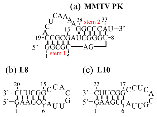
Figure 1: Secondary structures of studied RNA. Hairpins L8 and L10 have a 5’-pppG, while the MMTV PK does not have a phosphate group at the 5’-end.

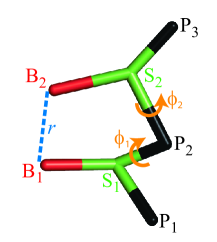
Figure 2: Illustration of the structural parameters in Eq. (UST). Sites P, S and B are shown in black, green and red, respectively. The indices refer to different nucleotides. $r$ is the distance between bases ${\rm B}_{1}$ and ${\rm B}_{2}$ in angstroms, and $\phi_{1}({\rm P}_{1},{\rm S}_{1},{\rm P}_{2},{\rm S}_{2})$ and $\phi_{2}({\rm P}_{3},{\rm S}_{2},{\rm P}_{2},{\rm S}_{1})$ are the dihedral angles in radians.

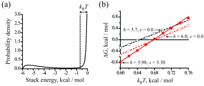
Figure 3: (a) A sample distribution of stacking energies $U_{\rm ST}$ (Eq. (UST)) from simulations of coarse-grained dimers. All dimer configurations with $U_{\rm ST}<-k_{\rm B}T$ are counted as stacked in Eq. (eqn:dGsim). (b) The free energy, $\Delta G$, of stack formation in dimer ${\rm G}\choose{\rm A}$, calculated using Eq. (eqn:dGsim) with $\Delta G_{0}=0$. Open and closed symbols show $\Delta G$ for different $U_{\rm ST}^{0}=-h+k_{\rm B}(T-T_{\rm m})s$, where $T_{\rm m}$ is the melting temperature of ${\rm G}\choose{\rm A}$ in Table tbl:table1 and $h$, $s$ vary. Red solid line shows $\Delta G=\Delta H-T\Delta S$ for $\Delta H$ and $\Delta S$ given in Table tbl:table1. Same $\Delta G$ is obtained in simulation with $h=5.98$ kcal/mol and $s=5.30$ (closed symbols).

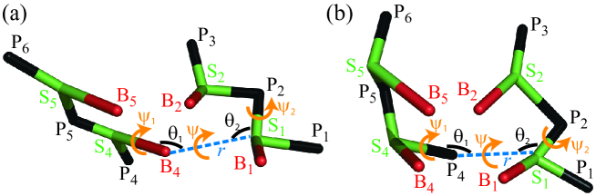
Figure 4: Illustration of the structural parameters in Eq. (UHB). Angle definitions depend on the site (P, S or B) which forms a hydrogen bond. Examples show hydrogen bonding between sites B and S (a) and between sites P and S (b). In (a), $r$ (S1, B4) is distance, $\theta_{1}$ (S4, B4, S1) and $\theta_{2}$ (P2, S1, B4) are angles, $\psi$ (P2, S1, B4, S4), $\psi_{1}$ (S1, B4, S4, P5) and $\psi_{2}$ (B4, S1, P2, S2) are dihedral angles. In (b), $r$ (S1, P4) is distance, $\theta_{1}$ (S4, P4, S1) and $\theta_{2}$ (P2, S1, P4) are angles, $\psi$ (P2, S1, P4, S4), $\psi_{1}$ (S1, P4, S4, P5) and $\psi_{2}$ (P4, S1, P2, S2) are dihedral angles. All other designations are the same as in Figure STACK.

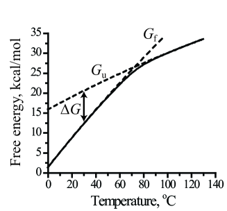
Figure 5: Geometrical definition of the stability $\Delta G(T)$ of the folded state. The solid curve shows the total free energy of the system $G(T)$, given by Eq. (GT4). The free energies of the folded and unfolded states, $G_{\rm f}(T)$ and $G_{\rm u}(T)$, are estimated from Eq. (GT5) using $T^{*}=0$ ^∘C and 130 ^∘C, respectively (dashed curves).

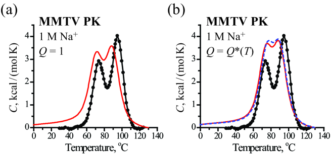
Figure 6: Measured⁴¹ (black symbols) and computed (red curve) heat capacity $C$ of the MMTV PK in 1 M Na⁺. The computed $C(T)$ is shown with respect to the heat capacity of the unfolded state at 130 ^∘C. $\Delta G_{0}=0.6$ kcal/mol, $U_{\rm{HB}}^{0}=2.43$ kcal/mol. In (a), $Q=1$. In (b), $Q=Q^{*}(T)$, $b=4.4$ Å. The blue dashed curve in (b) shows $C(T)$ from simulation using the solvent viscosity which is ten times larger than the $\eta$ specified in Methods. It can be rigorously established that the thermodynamic properties must be independent of $\eta$. In accord with this expectation simulations at high and low values of $\eta$ are in good agreement with each other despite the difficulty in obtaining adequate sampling for large $\eta$.

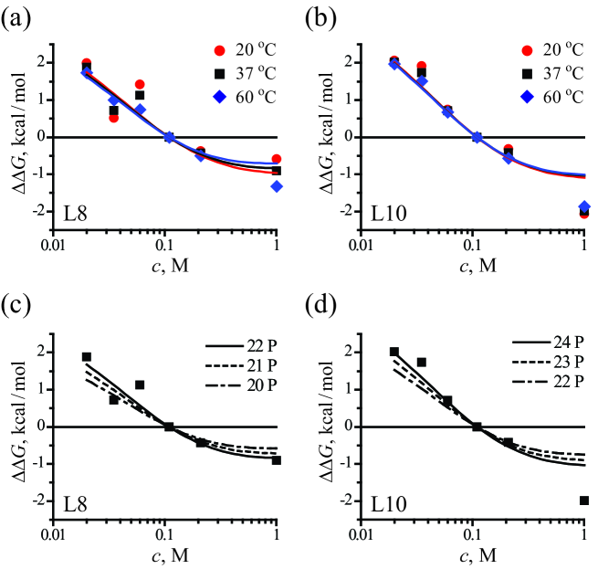
Figure 7: The stability $\Delta G$ of hairpins L8 and L10 as a function of salt concentration $c$, plotted as $\Delta\Delta G(c)=\Delta G(c)-\Delta G(c_{0})$, where $c_{0}=0.11$ M. Panels (a) and (b) show comparison of experiment (symbols) and simulation (curves) at different temperatures, assuming no hydrolysis of the 5’-pppG. Panels (c) and (d) illustrate the contribution of the 5’-pppG to $\Delta\Delta G(c)$ at 37 ^∘C for different levels of hydrolysis: no hydrolysis (solid), partial hydrolysis (dashed) and complete hydrolysis (dash-dotted). Simulation curves are for $Q=Q^{*}(T)$, $b=4.4$ Å.

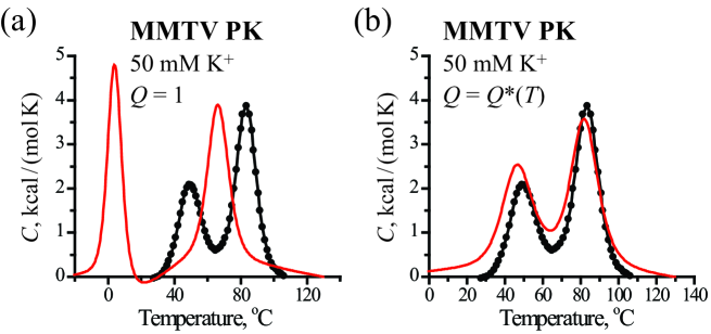
Figure 8: Same as in Figure VPK_c1 but in 50 mM K⁺.

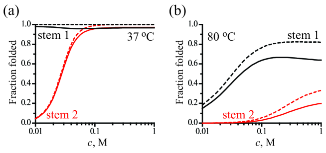
Figure 9: The fraction of folded stem 1 (black) and stem 2 (red) in the MMTV PK, as a function of salt concentration $c$. A stem is folded if five base pairs have formed (solid lines) or if one base pair has formed (dashed lines). $\Delta G_{0}=0.6$ kcal/mol, $U_{\rm{HB}}^{0}=2.43$ kcal/mol, $Q=Q^{*}(T)$, $b=4.4$ Å. In (a), $T=37$ ^∘C. In (b), $T=80$ ^∘C.

References

- Doudna and Cech 2002 Doudna, J. A.; Cech, T. R. Nature 2002, 418, 222–228
- Treiber and Williamson 1999 Treiber, D. K.; Williamson, J. R. Curr. Opin. Struct. Biol. 1999, 9, 339–345
- Thirumalai and Hyeon 2005 Thirumalai, D.; Hyeon, C. Biochemistry 2005, 44, 4957–4970
- Chen 2008 Chen, S.-J. Annu. Rev. Biophys. 2008, 37, 197–214
- Woodson 2011 Woodson, S. A. Acc. Chem. Res. 2011, 44, 1312–1319
- Zhuang et al. 2000 Zhuang, X.; Bartley, L.; Babcock, A.; Russell, R.; Ha, T.; Hershlag, D.; Chu, S. Science 2000, 288, 2048–2051
- Russell and Herschlag 2001 Russell, R.; Herschlag, D. J. Mol. Biol. 2001, 308, 839–851
- Thirumalai and Woodson 1996 Thirumalai, D.; Woodson, S. A. Acc. Chem. Res. 1996, 29, 433–439
- Tinoco and Bustamante 1999 Tinoco, I., Jr.; Bustamante, C. J. Mol. Biol. 1999, 293, 271–281
- Woodson 2005 Woodson, S. A. Curr. Opin. Chem. Biol. 2005, 9, 104–109
- Tan and Chen 2010 Tan, Z.-J.; Chen, S.-J. Biophys. J. 2010, 99, 1565–1576
- Hyeon and Thirumalai 2005 Hyeon, C.; Thirumalai, D. Proc. Natl. Acad. Sci. U.S.A 2005, 102, 6789–6794
- Tan and Chen 2011 Tan, Z.-J.; Chen, S.-J. Biophys. J. 2011, 101, 176–187
- Kirmizialtin et al. 2012 Kirmizialtin, S.; Pabit, S. A.; Meisburger, S. P.; Pollack, L.; Elber, R. Biophys. J. 2012, 102, 819–828
- Tan and Chen 2008 Tan, Z.-J.; Chen, S.-J. Biophys. J. 2008, 95, 738–752
- Ha and Thirumalai 2003 Ha, B. Y.; Thirumalai, D. Macromolecules 2003, 36, 9658–9666
- Chen et al. 2012 Chen, K.; Eargle, J.; Lai, J.; Kim, H.; Abeysirigunawardena, S.; Mayerle, M.; Woodson, S.; Ha, T.; Luthey-Schulten, Z. J. Phys. Chem. B 2012, 116, 6819–6831
- Thirumalai et al. 2001 Thirumalai, D.; Lee, N.; Woodson, S. A.; Klimov, D. K. Annu. Rev. Phys. Chem. 2001, 52, 751–762
- Koculi et al. 2006 Koculi, E.; Thirumalai, D.; Woodson, S. A. J. Mol. Biol. 2006, 359, 446–454
- Koculi et al. 2007 Koculi, E.; Hyeon, C.; Thirumalai, D.; Woodson, S. A. J. Am. Chem. Soc. 2007, 129, 2676–2682
- Whitford et al. 2009 Whitford, P. C.; Schug, A.; Saunders, J.; Hennelly, S. P.; Onuchic, J. N.; Sanbonmatsu, K. Y. Biophys. J. 2009, 96, L7–L9
- Cho et al. 2009 Cho, S. S.; Pincus, D. L.; Thirumalai, D. Proc. Natl. Acad. Sci. U.S.A 2009, 106, 17349–17354
- Lin and Thirumalai 2008 Lin, J.; Thirumalai, D. J. Am. Chem. Soc. 2008, 130, 14080–14081
- Feng et al. 2011 Feng, J.; Walter, N. G.; Brooks, C. L., III J. Am. Chem. Soc. 2011, 133, 4196–4199
- Denesyuk and Thirumalai 2011 Denesyuk, N. A.; Thirumalai, D. J. Am. Chem. Soc. 2011, 133, 11858–11861
- 26 A sample A-form RNA structure can be found at http://www.biochem.umd.edu/ biochem/kahn/teach_res/dna_tutorial/.
- Chandler et al. 1983 Chandler, D.; Weeks, J. D.; Andersen, H. C. Science 1983, 220, 787–794
- Theimer et al. 2005 Theimer, C. A.; Blois, C. A.; Feigon, J. Mol. Cell 2005, 17, 671–682
- Xia et al. 1998 Xia, T.; SantaLucia, J., Jr.; Burkand, M. E.; Kierzek, R.; Schroeder, S. J.; Jiao, X.; Cox, C.; Turner, D. H. Biochemistry 1998, 37, 14719–14735
- Bloomfield et al. 2000 Bloomfield, V. A.; Crothers, D. M.; Tinoco, I., Jr. Nucleic Acids: Structures, Properties, and Functions, 1st ed.; University Science Books, 2000
- Dima et al. 2005 Dima, R. I.; Hyeon, C.; Thirumalai, D. J. Mol. Biol. 2005, 347, 53–69
- Florián et al. 1999 Florián, J.; Šponer, J.; Warshel, A. J. Phys. Chem. B 1999, 103, 884–892
- Shen and Tinoco 1995 Shen, L. X.; Tinoco, I., Jr. J. Mol. Biol. 1995, 247, 963–978
- Manning 1969 Manning, G. S. J. Chem. Phys. 1969, 51, 924–933
- Heilman-Miller et al. 2001 Heilman-Miller, S. L.; Thirumalai, D.; Woodson, S. A. J. Mol. Biol. 2001, 306, 1157–1166
- Sharp and Honig 1990 Sharp, K. A.; Honig, B. J. Phys. Chem. 1990, 94, 7684–7692
- Hasted 1972 Hasted, J. B. Liquid water: dielectric properties; Water, a Comprehensive Treatise; Plenum Press: New York, 1972; Vol. 1; pp 255–309
- Williams and Hall 1996 Williams, D. J.; Hall, K. B. Biochemistry 1996, 35, 14665–14670
- Mikulecky and Feig 2006 Mikulecky, P. J.; Feig, A. L. Biopolymers 2006, 82, 38–58
- Honeycutt and Thirumalai 1992 Honeycutt, J. D.; Thirumalai, D. Biopolymers 1992, 32, 695–709
- Theimer and Giedroc 2000 Theimer, C. A.; Giedroc, D. P. RNA 2000, 6, 409–421
- Manning 1976 Manning, G. S. Biopolymers 1976, 15, 2385–2390
- Record et al. 1976 Record, M. T., Jr.; Woodbury, C. P.; Lohman, T. M. Biopolymers 1976, 15, 893–915
- Bond et al. 1994 Bond, J. P.; Anderson, C. F.; Record, M. T., Jr. Biophys. J. 1994, 67, 825–836