Study of Standard Model Scalar Production in Bosonic Decay Channels in CMS

The status of the Standard Model Scalar Boson search in the bosonic decay channels at the CMS experiment at the LHC is presented. The results are based on proton-proton collisions data corresponding to integrated luminosities of up to 5.1 $\mathrm{fb^{-1}}$ at $\sqrt{s}$ = 7 $\mathrm{Te\kern-0.80005ptV}$ and 19.6 $\mathrm{fb^{-1}}$ at $\sqrt{s}$ = 8 $\mathrm{Te\kern-0.80005ptV}$. The observation of a new boson at a mass near 126 $\mathrm{Ge\kern-0.80005ptV}$ is confirmed by the analysis of the new data and first measurements of the boson properties are shown.

1 Introduction

One of the open questions in the standard model (SM) of particle physics $\!{}^{{\bf?},{\bf?},{\bf?}}$ is the origin of the masses of fundamental particles. Within the SM, vector boson masses arise from the spontaneous breaking of electroweak symmetry by the Higgs field $\!{}^{{\bf?},{\bf?},{\bf?},{\bf?},{\bf?},{\bf?}}$. In 2012, the LHC experiments, ATLAS and CMS, reported the discovery of a new boson at approximately 125 $\mathrm{Ge\kern-1.00006ptV}$with 5 or more standard deviations each $\!{}^{{\bf?},{\bf?}}$. Both observations are consistent with expectations for the SM Higgs boson within the large statistical uncertainties.

The $\mathrm{H}\to VV$ modes have the largest sensitivity among all Higgs decays. In particular, the $\mathrm{H}\to\mathrm{Z}\mathrm{Z}\to 4\ell$ and $\mathrm{H}\to\gamma\gamma$ modes have very good mass resolution, while the $\mathrm{H}\to\mathrm{W}\mathrm{W}\to 2\ell 2\nu$ mode has very large signal yield. In these proceedings the updated analyses with the full available dataset by the time of the conference are summarized. The data sample corresponds up to 5.1 $\pm$ 0.1 $\mathrm{fb^{-1}}$ (19.5 $\pm$ 0.8 $\mathrm{fb^{-1}}$) of integrated luminosity collected in 2011 (2012) at a center-of-mass energy of 7 (8) $\mathrm{Te\kern-1.00006ptV}$ collected by the CMS experiment at the LHC.

These proceedings are organized as follows. Section 2 briefly describes the main components of the CMS detector used in the analyses, while Section 3 describes the general selection used to define the objects. The following Sections 4 to 7 explain each updated final state analysis: $\mathrm{H}\to\mathrm{Z}\mathrm{Z}\to 4\ell$, $\mathrm{H}\to\mathrm{W}\mathrm{W}\to 2\ell 2\nu$, $\mathrm{W}\mathrm{H}\to\mathrm{W}\mathrm{W}\mathrm{W}\to 3\ell 3\nu$ and $\mathrm{H}\to\mathrm{Z}\gamma$. It is worth noting the spin and parity studies on $\mathrm{H}\to\mathrm{Z}\mathrm{Z}\to 4\ell$ and $\mathrm{H}\to\mathrm{W}\mathrm{W}\to 2\ell 2\nu$ are summarized in the CMS Standard Model Scalar properties proceeding. By the time of the conference, there was no update on $\mathrm{H}\to\gamma\gamma$, and therefore the quoted results in Reference $\!{}^{{\bf?}}$ were still valid.

All Higgs production mechanisms are considered: the gluon fusion process, the associated production of the Higgs boson with a $\mathrm{W}$ or $\mathrm{Z}$ boson (VH), the $\mathrm{t}\bar{\mathrm{t}}\mathrm{H}$ process, and the vector boson fusion (VBF) process. The SM Higgs boson production cross sections are taken from Reference $\!{}^{{\bf?}}$.

2 CMS detector and event simulation

The CMS detector is described in detail elsewhere $\!{}^{{\bf?}}$. The key components used for this analysis are summarized here. A superconducting solenoid occupies the central region of the CMS detector, providing an axial magnetic field of 3.8 Tesla parallel to the beam direction. Charged particle trajectories are measured by the silicon pixel and strip tracker, which cover the pseudo-rapidity region $|\eta|<2.5$. Here, $\eta$ is defined as $\eta=-\ln{\tan{\theta/2}}$, where $\theta$ is the polar angle of the trajectory of the particle with respect to the direction of the counterclockwise beam. A crystal electromagnetic calorimeter (ECAL) and a brass/scintillator hadron calorimeter (HCAL) surround the tracking volume and cover $|\eta|<3$. A quartz-fiber Cherenkov calorimeter (HF) extends the coverage to $|\eta|<5$. The muon system consists of gas detectors embedded in the iron return yoke outside the solenoid, with a coverage to $|\eta|<2.4$. The first level of the CMS trigger system, composed of custom hardware processors, is designed to select the most interesting events in less than 3 $\mu s$, using information from the calorimeters and muon detectors. The High Level Trigger processor farm further reduces the event rate to a few hundred Hz before data storage.

Several Monte Carlo event generators are used to simulate the signal and background processes. For all of them, the detector response is simulated using a detailed description of the CMS detector, based on the geant4 package $\!{}^{{\bf?}}$. Minimum bias events are superimposed on the simulated events to emulate the additional pp interactions per bunch crossing (pile-up). These samples are re-weighted to represent the pile-up distribution as measured in the data. The average number of pile-up events per beam crossing in the 2011 data is about 10, and in the 2012 data it is about 20.

3 Object selection

The selection requirements to define the objects in the different final states depend on their specific characteristics, both in terms of the signal topology and the background processes. Nevertheless, the general strategy to select the different objects is common for all of them, and it is described below.

Signal candidates are selected online by trigger paths requiring the presence of one or several electrons or muons. The use of a combination of them make the efficiencies for events satisfying the analysis selection above 95% for the final states under study.

Muon candidates are reconstructed combining two algorithms, one in which tracks in the silicon detector are matched to hits in the muon system, and another in which a global fit is performed on hits in both the silicon tracker and the muon system. Muons are required to be isolated to distinguish between muons from $\mathrm{W}/\mathrm{Z}$ boson decays and those from QCD background processes, which are usually in or near jets. For each muon candidate, the scalar sum of the transverse energy of all particles compatible with originating from the primary vertex is reconstructed in cones of several widths around the muon direction, excluding the contribution from the muon itself. This information is combined using a multivariate algorithm which exploits the differences in the differential energy deposition between prompt muons and muons from hadron decays inside a jet, to discriminate between signal and background.

Electron candidates are identified using a multivariate approach based on variables which exploit information from the tracker, the ECAL, and the combination of these two detectors. Electron isolation is characterized by the ratio of the sum of the transverse energy of the particles reconstructed in a cone around the electron, excluding the contribution from the electron itself, and the transverse energy of the electron. Isolated electrons are selected by requiring this ratio to be below a threshold.

For both electrons and muons corrections are applied to account for the contribution to the energy in the isolation cone from the pile-up. A median energy density ($\rho$) is determined event by event and the pile-up contribution is estimated as the product of $\rho$ and an effective isolation cone area. This contribution is subtracted $\!{}^{{\bf?}}$ from the transverse energy in the isolation cone.

Hadronically decaying $\tau$ leptons are reconstructed and identified using an algorithm $\!{}^{{\bf?}}$ which targets the main decay modes by selecting candidates with one charged hadron and up to two neutral pions, or with three charged hadrons.

The lepton candidates are required to originate from the primary vertex of the event, which is chosen as the vertex with the highest $\sum p_{\mathrm{T}}^{2}$, where the sum runs over all tracks associated with the vertex.

Photon candidates are reconstructed from clusters of channels in the ECAL around channels with significant energy deposits, which are merged into superclusters. The clustering algorithms result in almost complete recovery of the energy of photons in spite of the large fraction of Bremsstrahlung and converted photons. In the endcaps, the preshower energy is added where the preshower is present ($|\eta|>1.65$). The observables used in the photon selection are: isolation variables based on the particle flow algorithm $\!{}^{{\bf?}}$, the ratio of hadronic energy in the hadron calorimeter towers behind the supercluster to the electromagnetic energy in the supercluster, the transverse width of the electromagnetic shower, and an electron veto to avoid misidentifying an electron as a photon.

Jets are reconstructed using the anti-$\mathrm{k_{T}}$ clustering algorithm $\!{}^{{\bf?}}$ with distance parameter $\Delta\mathrm{R}=0.5$, as implemented in the fastjet package $\!{}^{{\bf?}}$. A similar correction as for the lepton isolation is applied to account for the contribution to the jet energy from pile-up events. Jet energy corrections are applied as a function of the jet $E_{\mathrm{T}}$ and $\eta$ $\!{}^{{\bf?}}$. Events are classified according to the number of selected jets with $E_{\mathrm{T}}>30~{}\mathrm{Ge\kern-1.00006ptV}$ and $|\eta|<~{}4.7$.

Neutrinos escape detection, and result in large missing transverse energy, $E_{\mathrm{T}}^{\mathrm{miss}}$, defined as the modulus of the negative vector sum of the transverse momenta of all reconstructed particles (charged or neutral) in the event $\!{}^{{\bf?}}$. Since the $E_{\mathrm{T}}^{\mathrm{miss}}$ resolution is degraded by pile-up, the minimum of two different observables is used. The first includes all particle candidates in the event $\!{}^{{\bf?}}$. The second uses only the charged particle candidates associated with the primary vertex. The use of both variables exploits the presence of a correlation between the two variables in signal events with genuine $E_{\mathrm{T}}^{\mathrm{miss}}$, and its absence otherwise, as in Drell-Yan events.

To suppress the top-quark background, a top tagging technique based on soft-muon and b-jet tagging $\!{}^{{\bf?}}$ is applied. The first method rejects events with soft muons which likely come from semileptonic b-decays coming from top-quark decays. The second method uses a b-jet tagging algorithm which looks for tracks with large impact parameter within jets. For the second method jets with $E_{\mathrm{T}}>15~{}\mathrm{Ge\kern-1.00006ptV}$ are considered. The rejection factor for the top-quark background is about 50% in the 0-jet category and above 80% for events with at least one jet passing the selection criteria.

4 $\mathrm{H}\to\mathrm{Z}\mathrm{Z}\to 4\ell$ analysis

The $\mathrm{H}\to\mathrm{Z}\mathrm{Z}\to 4\ell$ analysis $\!{}^{{\bf?}}$ presented here relies critically on the reconstruction, identification, and isolation of leptons. The high lepton reconstruction efficiencies are achieved for a $\mathrm{Z}\mathrm{Z}$ system composed of two pairs of same-flavour and opposite-charge isolated leptons, in the measurement range $m_{4\ell},m_{2\ell 2\tau}>100~{}\mathrm{Ge\kern-1.00006ptV}$. One or both of the $\mathrm{Z}$ bosons can be off-shell. The background sources include an irreducible four-lepton contribution from direct $\mathrm{Z}\mathrm{Z}$ (or $\mathrm{Z}\gamma^{*}$) production via $qq$ annihilation and $gg$ fusion. Reducible contributions arise from $\mathrm{Z}+b\bar{b}$ and $\mathrm{t}\bar{\mathrm{t}}$, where the final states contain two isolated leptons and two jets producing secondary leptons. Additional background of instrumental nature arises from $\mathrm{Z}+jets$, $\mathrm{Z}+\gamma+jets$ and $\mathrm{W}\mathrm{Z}+jets$ events, where jets are misidentified as leptons.

A matrix element likelihood approach $\!{}^{{\bf?},{\bf?},{\bf?}}$ is used to construct a kinematic discriminant ($K_{D}$) based on the probability ratio of the signal and background hypotheses, $K_{D}={\cal P_{\mathrm{sig}}}/({\cal P_{\mathrm{sig}}}+{\cal P_{\mathrm{bkg}}})$, where the likelihood ratio is defined for each value of $m_{4\ell}$, being $P_{\mathrm{sig}}$ and $P_{\mathrm{bkg}}$ the signal and background probabilities, respectively.

To improve the sensitivity to the production mechanisms, the event sample is split into two categories based on the jet multiplicity: events with fewer than two jets, and events with at least two jets. In the first category the transverse momentum divided by the mass of the four lepton system ($p_{\mathrm{T}}/m_{4\ell}$) is used to discriminate VBF and VH from gluon fusion. In the second category a linear discriminant ($V_{D}$) is formed combining two VBF sensitive variables, the difference in pseudo-rapidity and the invariant mass of the two leading jets. The discriminant is tuned to separate vector boson from gluon fusion processes.

In summary, $m_{4\ell}$, $K_{D}$, and the two distributions after splitting into two categories based on the jet multiplicity are used to discriminate between signal and background. The reconstructed four-lepton invariant-mass distributions for the $4\ell$ and $2\ell 2\tau$ final states are shown in Figure 1 and compared with the expectation from SM background processes. The observed distribution is in good agreement with the expectation. The $\mathrm{Z}\rightarrow 4\ell$ resonance peak is observed with normalization and shape as expected. The measured distribution at higher mass is dominated by the irreducible $\mathrm{Z}\mathrm{Z}$ background. A clear peak around $m_{4\ell}=126$ GeV is seen.

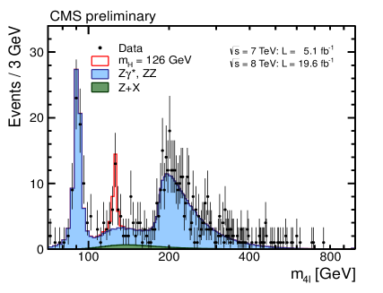
Figure 1: Distribution of the $4\ell$ (left) and $2\ell 2\tau$ (right) reconstructed mass in the full mass range. Points represent the data, shaded histograms represent the background and unshaded histogram the signal expectation.

The distributions of the kinematic discriminant $K_{D}$ versus $m_{4\ell}$ are shown for the selected events and compared to SM background expectation in Figure 2. The distributions of $p_{\mathrm{T}}/m_{4\ell}$ and the VBF discriminant $V_{D}$ are presented in Figure 3.

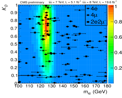
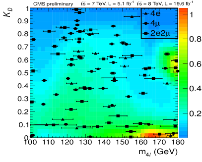
Figure 2: Distribution of the kinematic discriminant $K_{D}$ versus $m_{4\ell}$ in the low-mass region. The contours represent the expected relative density of signal events for $m_{\mathrm{H}}=126~{}\mathrm{Ge\kern-1.00006ptV}$ (left) and for background events (right). The points show data and measured invariant mass uncertainties as horizontal bars.

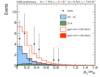
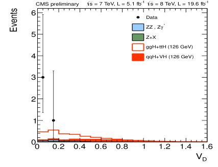
Figure 3: Distributions for the $p_{\mathrm{T}}/m_{4\ell}$ in the first category for the VBF discriminant in second category. Only events in the mass region $121.5<m_{4\ell}<130.5\mathrm{Ge\kern-1.00006ptV}$ are considered.

The local $p$-values, representing the significance of local excesses relative to the background expectation, are shown as a function of $m_{\mathrm{H}}$ in Figure 4. The minimum of the local $p$-value is reached around $m_{4\ell}=125.8$ GeV, and corresponds to a local significance of $6.7\sigma$ (for an expectation of 7.2 $\sigma$). This constitutes an observation of the new boson in the four-leptons channel alone. As a cross-check, the 1D ($m_{4\ell}$) and 2D ($m_{4\ell}$, $K_{D}$) models are also studied, and observed a local significance of 4.7 and 6.6 $\sigma$, for an expectation of 5.6 and 6.9 $\sigma$, respectively. The upper 95% confidence level (CL) limits obtained from the combination of the $4\ell$ and $2\ell 2\tau$ channels using the modified frequentist construction CL_s method $\!{}^{{\bf?},{\bf?},{\bf?}}$ are also shown in Figure 4. The SM-like Higgs boson is excluded by the four-lepton channels at 95% CL in the range 130–827 $\mathrm{Ge\kern-1.00006ptV}$ (for an expectation of 114–778 $\mathrm{Ge\kern-1.00006ptV}$). The signal strength $\mu$, relative to the expectation for the SM Higgs boson, is measured to be $\mu=0.91^{+0.30}_{-0.24}$ at 125.8 $\mathrm{Ge\kern-1.00006ptV}$.

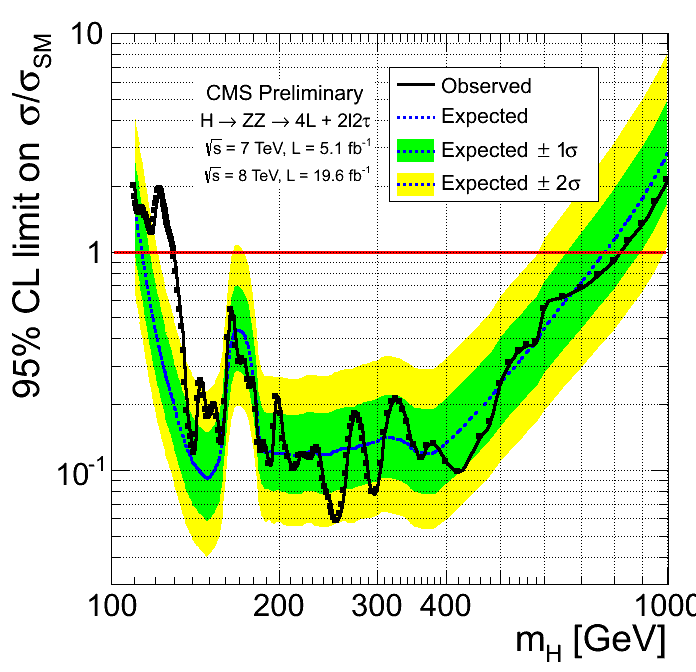
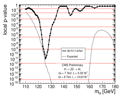
Figure 4: Observed and expected 95% CL upper limit (left) on the ratio of the production cross section to the SM expectation in the $\mathrm{H}\to\mathrm{Z}\mathrm{Z}\to 4\ell$ analysis. The 68% and 95% ranges of expectation for the background-only model are also shown with green and yellow bands, respectively. Significance of the local excess (right) with respect to the SM background expectation as a function of the Higgs boson mass.

The mass measurement of the new resonance is performed with a three-dimensional fit using for each event the four-lepton invariant mass, the associated per-event mass uncertainty, and the kinematic discriminant. Per-event uncertainties on the four-lepton invariant mass are calculated from the individual lepton momentum uncertainties. Figure 5 shows the one-dimensional likelihood scan versus SM Higgs boson mass performed under the assumption that its width is much smaller than the detector resolution. The resulting fit gives $m_{\rm H}=125.8\pm 0.5$ (stat.) $\pm 0.2$ (syst.) GeV. The systematic uncertainty accounts for the effect on the mass scale of the lepton momentum scale and resolution.

The jet categorization and the utilization of the transverse momentum spectrum and vector boson fusion sensitive variables are used to disentangle the production mechanisms of the observed new state. The production mechanisms are split into two categories depending on whether the production is induced by vector bosons (VBF, VH) or fermions (gluon fusion loop with quarks, $\mathrm{t}\bar{\mathrm{t}}\mathrm{H}$). Two respective signal strength modifiers ($\mu_{F},\mu_{V}$) are introduced as scale factors to the SM expected cross section. A two dimensional fit is performed for the two signal strength modifiers assuming a mass hypothesis of $m_{H}=125.8~{}\mathrm{Ge\kern-1.00006ptV}$. Figure 5 shows the result of the ($\mu_{V},\mu_{F}$) fit, leading to the measurements $\mu_{V}=1.0^{+2.4}_{-2.3}$ and $\mu_{F}=0.9^{+0.5}_{-0.4}$.

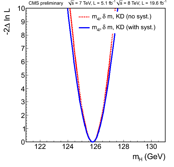
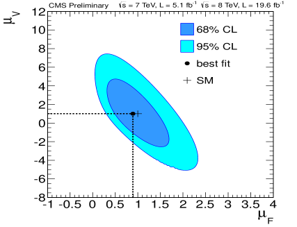
Figure 5: 1D test statistics q($m_{\mathrm{H}}$)=$-2\Delta\ln{\rm L}$ scan vs tested Higgs boson mass $m_{\mathrm{H}}$, obtained from the 3D test statistics profiling the minimum of the signal strengths, with and without systematics (left). Likelihood contours on the signal strength modifiers associated with fermions ($\mu_{F}$) and vector bosons ($\mu_{V}$) shown at 68% and 95% CL (right).

5 $\mathrm{H}\to\mathrm{W}\mathrm{W}\to 2\ell 2\nu$ analysis

The search strategy for $\mathrm{H}\to\mathrm{W}^{+}\mathrm{W}^{-}$ is based on the final state in which both $\mathrm{W}$ bosons decay leptonically $\!{}^{{\bf?}}$, resulting in a signature with two isolated, oppositely charged, high $p_{\mathrm{T}}$ leptons (electrons or muons) and large missing transverse momentum, $E_{\mathrm{T}}^{\mathrm{miss}}$, due to the undetected neutrinos.

To improve the signal sensitivity, the events are separated according to lepton flavor into $\mathrm{\mathrm{e}}^{+}\mathrm{\mathrm{e}}^{-}$, $\mu^{+}\mu^{-}$, and $\mathrm{\mathrm{e}}^{\pm}\mu^{\mp}$ samples and according to jet multiplicity into 0-jet and 1-jet samples.

To reduce the background from $\mathrm{W}\mathrm{Z}$ production, any event that has a third lepton passing the identification and isolation requirements is rejected. The contribution from $W\gamma$ production, when the photon is misidentified as an electron, is reduced by about 90% in the dielectron final state by $\gamma$ conversion rejection requirements. The background from low mass resonances is rejected by requiring a dilepton mass ($m_{\mathrm{\ell}\mathrm{\ell}}$) greater than 12 $\mathrm{Ge\kern-1.00006ptV}$. A minimum requirement on the dilepton transverse momentum ($p_{\mathrm{T}}^{\ell\ell}$) is applied to reduce the $\mathrm{W+jets}$ background.

The Drell-Yan process produces same-flavor lepton pairs ($\mathrm{\mathrm{e}}^{+}\mathrm{\mathrm{e}}^{-}$ and $\mu^{+}\mu^{-}$). In order to suppress this background, a few additional cuts are applied in the same-flavor final states. First, the resonant component of the Drell-Yan production is rejected by requiring a dilepton mass outside a 30 $\mathrm{Ge\kern-1.00006ptV}$ window centered on the $\mathrm{Z}$ pole. Then, the remaining off-peak contribution is suppressed by exploiting different $E_{\mathrm{T}}^{\mathrm{miss}}$-based approaches.

To enhance the sensitivity to a Higgs boson signal, a cut-based approach is chosen for the final “Higgs” selection in all categories. Because the kinematics of signal events change as a function of the Higgs mass, separate optimizations are performed for different $m_{\mathrm{H}}$ hypotheses in a cut–based analysis. In addition, a two-dimensional shape analysis technique is also pursued for the different-flavor final state in the 0-jet and 1-jet categories. This second analysis is more sensitive to the presence of a Higgs boson and is used as a baseline for the final results.

In the cut-based approach extra requirements, designed to optimize the sensitivity for a SM Higgs boson, are placed on $p_{\mathrm{T}}^{\mathrm{\ell},\mathrm{max}}$, $p_{\mathrm{T}}^{\mathrm{\ell},\mathrm{min}}$, $m_{\mathrm{\ell}\mathrm{\ell}}$, $\Delta\phi_{\mathrm{\ell}\mathrm{\ell}}$ and the transverse mass $m_{\mathrm{T}}$, defined as $\sqrt{2p_{\mathrm{T}}^{\ell\ell}E_{\mathrm{T}}^{\mathrm{miss}}(1-\cos\Delta\phi_{E_{\mathrm{T}}^{\mathrm{miss}}\mathrm{\ell}\mathrm{\ell}})}$, where $\Delta\phi_{E_{\mathrm{T}}^{\mathrm{miss}}\mathrm{\ell}\mathrm{\ell}}$ is the difference in azimuth between $E_{\mathrm{T}}^{\mathrm{miss}}$ and the transverse momentum of the dilepton system. The $m_{\mathrm{\ell}\mathrm{\ell}}$ and $m_{\mathrm{T}}$ distributions in the 0-jet in the different-flavor final state are shown in Figure 6 for a SM Higgs boson with $m_{\mathrm{H}}=125~{}\mathrm{Ge\kern-1.00006ptV}$.

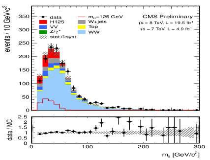
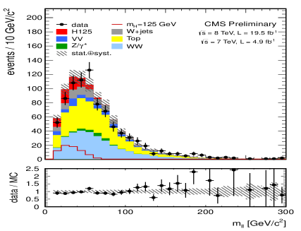
Figure 6: Distributions of dilepton mass (left) and the transverse mass (right) in the 0-jet category, in the different-flavor final state for a $m_{\mathrm{H}}=125~{}\mathrm{Ge\kern-1.00006ptV}$ SM Higgs boson and for the main backgrounds. The cut-based $\mathrm{H}\to\mathrm{W}^{+}\mathrm{W}^{-}$ selection, except for the requirement on the variable itself, is applied.

The two-dimensional shape analysis for the different-flavor final state uses two independent variables, $m_{\mathrm{T}}$ and $m_{\mathrm{\ell}\mathrm{\ell}}$. It allows for a simpler physical interpretation of the observed data with a sensitivity comparable to other more complex techniques. The two-dimensional distributions for the $m_{\mathrm{H}}=125~{}\mathrm{Ge\kern-1.00006ptV}$ Higgs signal hypothesis and background processes are shown in Figure 7 for the 0-jet bin.

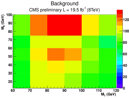
Figure 7: Two-dimensional $m_{T}-m_{\mathrm{\ell}\mathrm{\ell}}$ distributions in the 0-jet bin for the $m_{\mathrm{H}}=125~{}\mathrm{Ge\kern-1.00006ptV}$ SM Higgs signal hypothesis (left) and the background processes (right).

After applying the Higgs selection, upper limits are derived for the ratio of the product of the Higgs boson production cross section and the $\mathrm{H}\to\mathrm{W}^{+}\mathrm{W}^{-}$ branching fraction, $\sigma_{\mathrm{H}}\times\mathrm{BR}(\mathrm{H}\to\mathrm{W}^{+}\mathrm{W}^{-})$, and the SM Higgs expectation, $\sigma/\sigma_{SM}$. For the shape approach, the analysis in the different-flavor final state in the 0-jet and 1-jet categories is combined with the cut-based analysis in all other categories.

The 95% observed and median expected CL upper limits for the shape analysis are shown in Figure 8, which excludes a Higgs boson in the mass in the range 128–600 $\mathrm{Ge\kern-1.00006ptV}$ at 95% CL. The expected exclusion range for the background only hypothesis is 115–575 $\mathrm{Ge\kern-1.00006ptV}$. An excess of events is observed for hypothetical low Higgs boson masses, which makes the observed limits weaker than the expected ones. Due to the poor mass resolution of this channel the excess extends over a large mass range.

The observed (expected) significance for a SM Higgs with a mass of 125 $\mathrm{Ge\kern-1.00006ptV}$ is 4.0 (5.1) standard deviations for the shape-based analysis. The observed and expected significances and for each Higgs mass hypothesis is shown in Figure 8. The observed $\mu$ value for $m_{\mathrm{H}}=125~{}\mathrm{Ge\kern-1.00006ptV}$ using the shape-based analysis is 0.76 $\pm$ 0.13 (stat.) $\pm$ 0.16 (syst.) = 0.76 $\pm$ 0.21 (stat.+syst.). The statistical component is obtained by fixing all the nuisance parameters to their fit values and recomputing the likelihood profile. Then, the systematic component comes from a subtraction in quadrature of the full uncertainty and the statistical component.

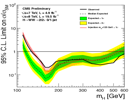
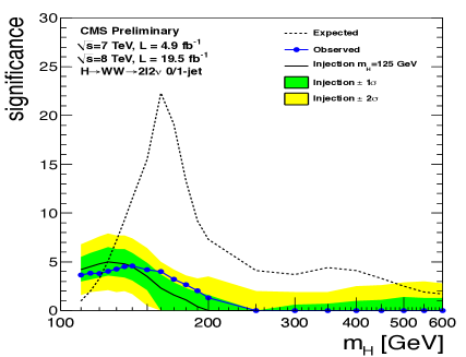
Figure 8: Expected and observed 95% CL upper limits on the cross section times branching fraction, $\sigma_{\mathrm{H}}\times\mathrm{BR}(\mathrm{H}\to\mathrm{W}^{+}\mathrm{W}^{-})$, relative to the SM Higgs expectation for the shape-based analysis (left). The expected limits in the presence of the Higgs with $m_{\mathrm{H}}=125\mathrm{Ge\kern-1.00006ptV}$ and its associated uncertainty are also shown. The observed and expected significances and for each Higgs mass hypothesis (right) for the shape-based analysis. The expected significance under the presence of a $m_{\mathrm{H}}=125\mathrm{Ge\kern-1.00006ptV}$ Higgs is also shown.

6 $\mathrm{W}\mathrm{H}\to\mathrm{W}\mathrm{W}\mathrm{W}\to 3\ell 3\nu$ analysis

In the $\mathrm{W}\mathrm{H}\to\mathrm{W}\mathrm{W}\mathrm{W}\to 3\ell 3\nu$ channel $\!{}^{{\bf?}}$, events are selected by requiring three charged lepton candidates, electrons or muons, with total charge equal to $\pm$1 are required, with $p_{\mathrm{T}}>$20 $\mathrm{Ge\kern-1.00006ptV}$ for the leading lepton and $p_{\mathrm{T}}>$10 $\mathrm{Ge\kern-1.00006ptV}$ for the other leptons. The data analysis is performed by using a shape-based approach, with a cross check from a single bin counting experiment. To further improve the sensitivity the events are split into two categories: all events that have an opposite-sign same-flavor lepton pair are classified in one category (OSSF), everything else is classified as in the same-sign same-flavor category (SSSF). While 1/4 of the events are selected in the second category, the expected background is rather small since physics processes leading to this final state have small cross section.

Events are required to have $E_{\mathrm{T}}^{\mathrm{miss}}$ above 40 (30) $\mathrm{Ge\kern-1.00006ptV}$ in the OSSF (SSSF) category. To reduce the background from top decays, events are rejected if there is at least one jet with $E_{\mathrm{T}}$ above 40 $\mathrm{Ge\kern-1.00006ptV}$. The $\mathrm{W}\mathrm{Z}\to 3\ell\nu$ background is largely reduced by requiring that all the OSSF lepton pairs have a dilepton mass at least 25 $\mathrm{Ge\kern-1.00006ptV}$ away from $m_{\mathrm{Z}}$. To reject the $\mathrm{Z}/\mathrm{W}+\gamma^{*}$ background, the dilepton mass of all opposite-charge lepton pairs are required to be greater than 12 $\mathrm{Ge\kern-1.00006ptV}$. Finally, the signal region is defined by requiring in addition to all the above cuts that the smallest dilepton mass $m_{\mathrm{\ell}\mathrm{\ell}}$ is less than 100 $\mathrm{Ge\kern-1.00006ptV}$ and that the smallest distance between opposite-charge leptons $\Delta R_{\ell^{+}\ell^{-}}$ is less than 2.

A shape-based analysis is carried out as a main analysis due to its superior performance with respect to a simple counting experiment. In this analysis a cut on $\Delta R_{\ell^{+}\ell^{-}}$ is not applied, and instead it is used as the final discriminant. Tests have shown this variable to provide the best discrimination between signal and background events, in terms of both expected limits and significance.

No significant excess of events is observed with respect to the background prediction, and 95% CL upper limits are calculated for the Higgs boson cross section with respect to $\sigma/\sigma_{SM}$. The expected and observed upper limits are shown in Figure 9. Since the analysis is independent of Higgs mass, and the shape of the $\Delta R_{\ell^{+}\ell^{-}}$ distribution changes just slightly for the Higgs signal, only small fluctuations are expected between different Higgs mass hypotheses. For the cut-based analysis, the observed (expected) upper limit at the 95% CL is 3.7 (3.6) times larger than the SM expectation for $m_{\mathrm{H}}=125~{}\mathrm{Ge\kern-1.00006ptV}$. For the shape-based analysis, the observed (expected) upper limit at the 95% CL is 3.3 (3.0) times larger than the SM expectation for $m_{\mathrm{H}}=125~{}\mathrm{Ge\kern-1.00006ptV}$.

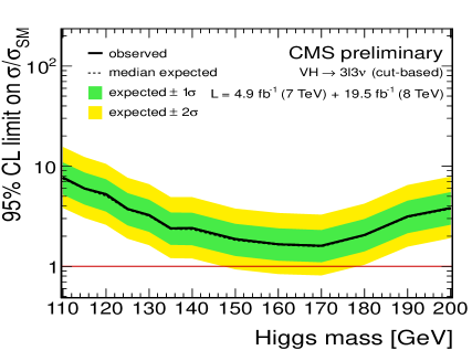
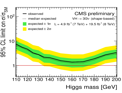
Figure 9: Upper limits at 95% CL in the $\mathrm{W}\mathrm{H}\to 3\ell 3\nu$ final state for the cut-based analysis (left) and shape-based analysis (right)

7 $\mathrm{H}\to\mathrm{Z}\gamma$ analysis

The $\mathrm{H}\to\mathrm{Z}\gamma$ decay channel $\!{}^{{\bf?}}$ is a clean final state, with the $\mathrm{Z}$ boson decaying into an electron or a muon pair, plus an isolated photon.

The invariant mass of at least one $\ell^{+}\ell^{-}$ pair is required to be greater than 50 $\mathrm{Ge\kern-1.00006ptV}$. If two dilepton pairs are present, the one closest to the $\mathrm{Z}$ mass is taken. The invariant mass of the $\ell^{+}\ell^{-}\gamma$ system, $m_{\ell\ell\gamma}$, is required to be between 100 and 180 $\mathrm{Ge\kern-1.00006ptV}$. Other conditions that combine the information from the photon and the leptons are: (1) the ratio of the photon transverse energy to $m_{\ell\ell\gamma}$ must be greater than 15/110, this requirement allows us to reject backgrounds without significant loss in signal sensitivity and without introducing a bias in the $m_{\ell\ell\gamma}$ spectrum; (2) the $\Delta R$ separation between each lepton and the photon must be greater than 0.4 in order to reject events with initial-state radiation avoiding photon influence lepton isolation; and (3) final-state radiation events are rejected by requiring a minimum of 185 GeV on the sum of $m_{\ell\ell\gamma}$ and $m_{\ell\ell}$.

The sensitivity of the search is enhanced by subdividing the selected events into classes according to indicators of the expected mass resolution and the signal-to-background ratio, and then combine the results in each class. For this purpose, four mutually exclusive event classes are defined: in terms of the pseudo-rapidity of the leptons and the photon and on the shower shape of the photon for one of the topologies. The background model fit to the $m_{\mu\mu\gamma}$ distribution for two event classes is shown in Figure 10.

No excess over the background is observed, and therefore the data are used to derive upper limits on the proton-proton Higgs boson production cross section times the $\mathrm{H}\to\mathrm{Z}\gamma$ branching fraction, $\sigma_{\mathrm{H}}\times\mathrm{BR}(\mathrm{H}\to\mathrm{Z}\gamma)$. The expected and observed limits are both shown in Figure 10. The expected exclusion limits at 95% confidence level are between 6 and 19 times the standard model cross section and the observed limit fluctuates between about 3 and 31 times the SM cross section.

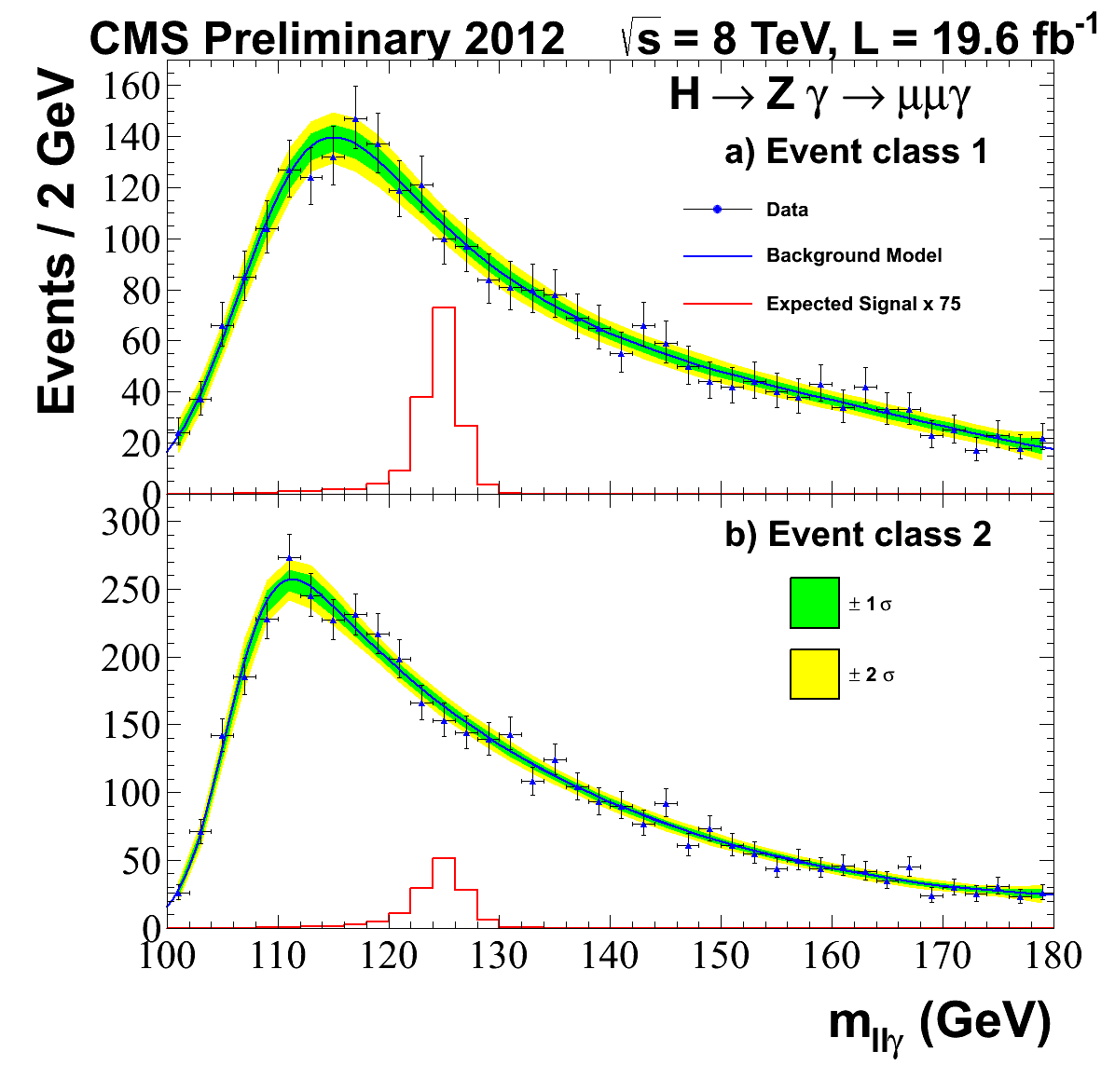
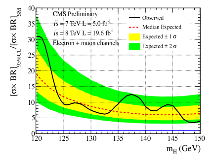
Figure 10: Background model fit to the $m_{\mu\mu\gamma}$ distribution for two event classes (left). The statistical uncertainty bands shown are computed from the data fit. Exclusion limit on the cross section of a SM Higgs boson decaying into $\mathrm{Z}$-boson and a photon as a function of $m_{\mathrm{H}}$ (right).

8 Summary

The status of the SM Scalar Boson search in the bosonic decay channels at the CMS experiment at the LHC has been presented. The results are based on proton-proton collisions data corresponding to integrated luminosities of up to 5.1 $\mathrm{fb^{-1}}$ at $\sqrt{s}$ = 7 $\mathrm{Te\kern-1.00006ptV}$ and 19.6 $\mathrm{fb^{-1}}$ at $\sqrt{s}$ = 8 $\mathrm{Te\kern-1.00006ptV}$. The observation of a new boson at a mass near 126 $\mathrm{Ge\kern-1.00006ptV}$ is confirmed by the analysis of the new data and first measurements of the boson properties have been shown.

References

References

- [1] ”Partial Symmetries of Weak Interactions”, Glashow, S. L., Nucl. Phys. 22, 579-588 (1961).
- [2] ”A Model of Leptons”, S. Weinberg,Phys. Rev. Lett. 19, 1264-1266 (1967).
- [3] ”Elementary particle physics: relativistic groups and analyticity”, A. Salam, Proceedings of the eighth Nobel symposium (1968).
- [4] ”Broken symmetries and the masses of gauge bosons”, F. Englert and R. Brout, Phys. Rev. Lett.. 13, 321-323 (1964).
- [5] ”Broken symmetries, massless particles and gauge fields”, P. Higgs, Phys. Rev. Lett.. 12, 132-133 (1964).
- [6] ”Broken symmetry and the mass of gauge vector mesons”, P. Higgs, Phys. Rev. Lett.. 13, 508 (1964).
- [7] ”Global conservation laws and massless particles”, Guralnik, G. S. and Hagen, C. R. and Kibble, T. W. B., Phys. Rev. Lett.. 13, 585-587 (1964).
- [8] ”Spontaneous symmetry breakdown without massless bosons”, P. Higgs, Phys. Rev. 145, 1156-1163 (1966).
- [9] ”Symmetry breaking in non-Abelian gauge theories”, Kibble, T. W. B., Phys. Rev. 155, 1554-1561 (1967).
- [10] ”Observation of a new boson at a mass of 125 GeV with the CMS experiment at the LHC”, CMS Collaboration, Phys.Lett. B716, 30-61 (2012).
- [11] ”Observation of a new particle in the search for the Standard Model Higgs boson with the ATLAS detector at the LHC”, ATLAS Collaboration, Phys.Lett. B716, 1-29 (2012).
- [12] ”Handbook of LHC Higgs Cross Sections: 1. Inclusive Observables”, LHC Higgs Cross Section Working Group, CERN-2011-002 (2011).
- [13] ”The CMS experiment at the CERN LHC”, CMS Collaboration, JINST 3, S08004 (2008).
- [14] ”GEANT4 A Simulation toolkit”, GEANT4 Collaboration, Nucl. Instrum. Meth. A506, 250 (2003).
- [15] ”Pile-up subtraction using jet areas”, M. Cacciari, G. P. Salam, Phys. Lett. B659, 119 (2008).
- [16] ”Performance of tau reconstruction algorithms in 2010 data collected with CMS”, CMS Collaboration, CMS-PAS-TAU-11-001 (2011).
- [17] ”Particle–Flow Event Reconstruction in CMS and Performance for Jets, Taus, and ”, CMS Collaboration, CMS-PAS-PFT-09-001 (2009).
- [18] ”Measurements of Inclusive W and Z Cross Sections in pp Collisions at TeV”, CMS Collaboration, JHEP 01, 080 (2011).
- [19] ”The anti- jet clustering algorithm”, M. Cacciari and G. P. Salam and G. Soyez, JHEP 04, 063 (2008).
- [20] ”Dispelling the myth for the jet-finder”, M. Cacciari, G. P. Salam, Phys. Lett. B641, 57 (2006).
- [21] ”Determination of Jet Energy Calibration and Transverse Momentum Resolution in CMS”, CMS Collaboration, JINST 6, 11002 (2011).
- [22] ”Algorithms for b Jet Identification in CMS”, CMS Collaboration, CMS-PAS-BTV-09-001 (2009).
- [23] ”Properties of the Higgs-like boson in the decay in pp collisions at and ”, CMS Collaboration, CMS-PAS-HIG-13-002 (2013).
- [24] ”Procedure for the LHC Higgs boson search combination in Summer 2011”, ATLAS and CMS Collaborations, CMS-NOTE-2011-005 (2011).
- [25] ”Presentation of search results: the CLs technique”, A. Read, J. Phys. G: Nucl. Part. Phys. 28, 2693 (2002).
- [26] ”Confidence level computation for combining searches with small statistics”, T. Junk, Nucl. Instrum. Meth. A 434, 435 (1999).
- [27] ”Update on the search for the standard model Higgs boson in pp collisions at the LHC decaying to in the fully leptonic final state”, CMS Collaboration, CMS-PAS-HIG-13-003 (2013).
- [28] ”Search for the Standard Model Higgs Boson in Decays”, CMS Collaboration, CMS-PAS-HIG-13-009 (2013).
- [29] ”Search for the standard model Higgs boson in the boson plus a photon channel in pp collisions at = 7 and 8 TeV”, CMS Collaboration, CMS-PAS-HIG-13-006 (2013).
- [30] ”MadGraph/MadEvent v4: The New Web Generation”, ”Alwall, Johan and others, JHEP 09, 028 (2007).
- [31] ”Precision Studies of the Higgs Golden Channel H ZZ* 4l. Part I. Kinematic discriminants from leading order matrix elements”, P. Avery, D. Bourilkov, M. Chen and others, CERN-PH-TH-2012-251 (2012).