Soft X-ray Fluxes of Major Flares Far Behind the Limb as Estimated Using STEREO EUV Images

Abstract

With increasing solar activity since 2010, many flares from the backside of the Sun have been observed by the Extreme Ultraviolet Imager (EUVI) on either of the twin STEREO spacecraft. Our objective is to estimate their X-ray peak fluxes from EUVI data by finding a relation of the EUVI with GOES X-ray fluxes. Because of the presence of the Fe xxiv line at 192 Å, the response of the EUVI 195 Å channel has a secondary broad peak around 15 MK, and its fluxes closely trace X-ray fluxes during the rise phase of flares. If the flare plasma is isothermal, the EUVI flux should be directly proportional to the GOES flux. In reality, the multithermal nature of the flare and other factors complicate the estimation of the X-ray fluxes from EUVI observations. We discuss the uncertainties, by comparing GOES fluxes with the high cadence EUV data from the Atmospheric Imaging Assembly (AIA) on board the Solar Dynamics Observatory (SDO). We conclude that the EUVI 195 Å data can provide estimates of the X-ray peak fluxes of intense flares (e.g., above M4 in the GOES scale) with uncertainties of a factor of a few. Lastly we show examples of intense flares from regions far behind the limb, some of which show eruptive signatures in AIA images.

1 Introduction

S-Introduction The Solar Terrestrial Relations Observatory (STEREO; Kaiser et al., 2008) was launched in October 2006, and continues to deliver unique views of the Sun not accessible from any Earth-bound instruments. STEREO consists of the Ahead (A) and Behind (B) spacecraft, which drift about 22^∘ a year in opposite directions from the Sun-Earth line. Both are equipped with nearly identical copies of the Extreme Ultraviolet Imager (EUVI; Wuelser et al., 2004) as part of the Sun Earth Connection Coronal and Heliospheric Investigation (SECCHI; Howard et al., 2008). In combination with images from the Atmospheric Imaging Assembly (AIA; Lemen et al., 2012) on board the Solar Dynamics Observatory (SDO; Pesnell, Thompson, and Chamberlin, 2012) we have observed the full longitudes of the solar corona in EUV since February 2011.

With the increasing separation of STEREO from the Sun-Earth line together with increasing solar activity since 2010, the EUVI has observed many flares far behind the limb from Earth view. Their X-ray emission is therefore completely occulted by the limb, and one of the frequently asked questions is “what would be the magnitude of such a flare in soft X-rays?” Data from the GOES X-ray Sensor (XRS) have played a major role in our understanding of the physics of solar flares as they have been widely used to derive plasma parameters (e.g., Feldman et al., 1996; Battaglia, Grigis, and Benz, 2005; Ryan et al., 2012). The flare class defined by the peak flux in the 1 – 8 Å band is generally thought to be a good measure of the released energy. In particular, the so-called X-class ($F_{1-8}\mathrel{\hbox{\hbox to0.0pt{\hbox{\lower 4.0pt\hbox{$\sim$}}\hss}\hbox{$>$}}}10^{-4}$ W m^-2) flares are often treated with special interests (e.g., Sudol and Harvey, 2005; LaBonte, Georgoulis, and Rust, 2007), because they release enormous amount of energy, and some of them may have a higher potential to perturb the heliosphere.

In this article, we explore the possibility to use EUVI data to estimate the GOES X-ray peak fluxes of flares far behind the limb. The response of the EUVI with temperature is vastly different from that of the GOES XRS. However, during flares, one of the four channels, namely the one that encompasses the Fe xii complex at 195 Å ($\approx$1.5 MK), should observe emissions from mainly hot ($>$10 MK) plasma (see, for example, Dere and Cook Dere and Cook (1979) who derived a typical differential emission measure of flares) due to the Fe xxiv line at 192 Å, which has the peak temperature of 15 – 20 MK, depending on the assumed ionization equilibrium. Therefore we focus on this EUVI channel to estimate the X-ray flux. In the next section, the temperature response of the EUVI is compared to that of the AIA. In Section 3, we use AIA data to study the origin and extent of the uncertainties that limit the accuracy of our work. This is followed in Section 4 by our main objective of finding an empirical relation of the EUVI with the GOES XRS fluxes. In Section 5 we show examples of flares from the backside that are estimated to be intense. Some of them leave observable signatures in AIA data. We summarize the work in Section 6, which also lists items that may possibly improve this work.

2 Temperature Response

T_Resp

The EUVI observes the Sun in four channels of EUV passbands that are similar to those of the Extreme-ultraviolet Imaging Telescope (EIT; Delaboudinière et al., 1995) on the Solar and Heliospheric Observatory (SOHO). They are 171 Å (Fe ix, Fe x), 195 Å (Fe xii, Fe xxiv), 284 Å (Fe xv) and 304 Å (He ii). Their temperature responses are plotted in Figure 1 as solid lines. Those for the AIA are plotted as dashed lines. In order to gain more comprehensive understanding of the structures and dynamics of the corona and transition region, the AIA has three more EUV channels, namely 94 Å (Fe xviii), 131 Å (Fe viii, Fe xxi), and 335 Å (Fe xvi). Additionally, the AIA replaces the 284 Å channel used by previous missions with the 211 Å channel that contains the Fe xiv line, but the peak temperature is similar.

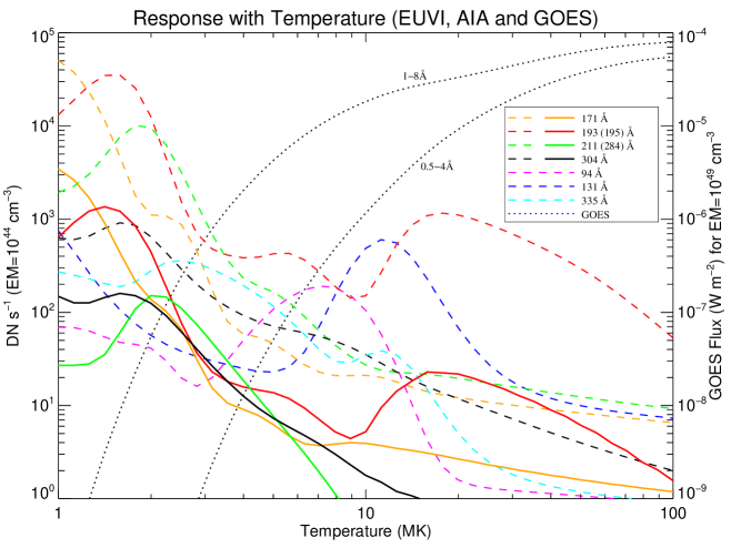
Figure 1.: Temperature response of EUVI on STEREO-A (solid lines), AIA (dashed lines) and GOES-14 (dotted lines). They are calculated using the CHIANTI atomic database version 7.0 (Dere et al., 1997; Landi et al., 2012). t˙resp˙euvi˙aia˙xrs

The two bands of the GOES XRS (plotted as dotted lines) have monotonically increasing response with temperature. Although none of these EUV channels has a similar temperature response, some of them have either primary or secondary peaks at high temperatures that characterize flares Dere and Cook (1979). Although AIA’s 131 Å channel (peaking at $\approx$10 MK) may be most often correlated with the XRS as indicated in the next section, it is clear that the 195 Å is the only EUVI channel that has a distinct peak of response above 10 MK. This broad peak around 15 MK is due to the Fe xxiv line at 192 Å. Therefore we use this channel exclusively for estimating the X-ray peak fluxes of flares not observed by GOES.

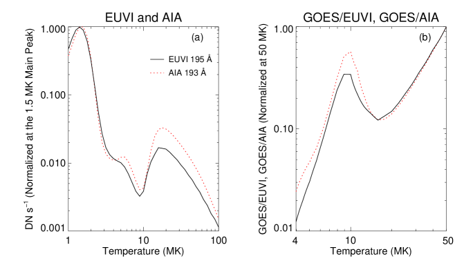
Figure 2.: (a) Comparison of EUVI’s 195 Å channel with AIA’s 193 Å channel, normalized at the respective primary peaks at $\approx$1.5 MK due to Fe xii. Because AIA’s passband is shifted to shorter wavelength, the secondary peak around 15 MK is more pronounced. (b) Although the GOES response monotonically increases with temperature (Figure 1), the ratio of GOES with AIA and EUVI has a dip due to the secondary peak of the latter instruments. t˙resp˙195

The high temperature response of the 195 Å channel is only secondary to the main peak at $\approx$1.5 MK. Figure 2 gives a closer view of the response of EUVI’s 195 Å channel in comparison with that of AIA’s 193 Å channel. We expect differences because AIA’s passband is shifted to shorter wavelengths. As the name indicates, the AIA channel’s effective area peaks at 193 Å rather than at 195 Å, and thus has a higher response at the wavelength of the Fe xxiv line. Figure 6 of Howard et al. Howard et al. (2008) and Figure 8 of Boerner et al. Boerner et al. (2012) give the effective areas of the EUVI and AIA, respectively. Specifically, the response to 15 MK plasma relative to the main response to 1.5 MK plasma is about a factor of two smaller for EUVI than for AIA (Figure 2(a)). The small difference of the effective area also affects the flux at a given temperature with respect to the GOES XRS flux. The GOES/EUVI and GOES/AIA ratios both decrease from 10 MK to 15 MK and increase above 15 MK, but reach the level of 10 MK at different temperatures as will be shown later in Figures 5 and 7. According to Figure 2(b), the GOES/AIA ratio at 35 MK is still small than that at 10 MK, whereas the GOES/EUVI ratio at 30 MK is already comparable to that at 10 MK.

3 AIA-GOES Relation

Data

In order to understand various uncertainties that may sometimes be critical in our objective of estimating the GOES X-ray peak flux from EUVI 195 Å data, we first compare light curves of flares from the AIA with those from the GOES XRS. The AIA takes images every 12 seconds in all the EUV channels, whereas the typical cadence of EUVI 195 Å images is 5 minutes. We select all flares above the GOES C3 ($F_{1-8}$ = 3$\times$10^-6 W m^-2) level between June 2010 and September 2012. In order to be free of the uncertainty from occultation by the limb, we limit to only those flares whose 2-D radial distance is less than 0.997$r_{\hbox{$\odot$}}$. We used the the Heliophysics Event Registry Hurlburt et al. (2012) for the flare locations.

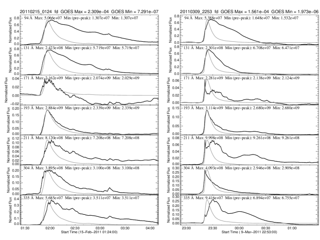
Figure 3.: Time variations of fluxes in AIA images. The channels plotted are (from top to bottom): 94 Å, 131 Å, 171 Å, 193 Å, 211 Å, 304 Å, and 335 Å. The preflare minimum is subtracted from each time profile. The GOES 1 – 8 Å light curves is overplotted in gray, scaled to [0,maximum] of each EUV light curve. two˙flares

Light curves are produced from the headers of individual level-1 full-disk images, which contain the average pixel values. To isolate the emission from the flare, we subtract the minimum flux during the 30 minute period preceding the GOES peak time. In Figure 3, we show two examples of the light curves. They are X-class flares (SOL2011-02-15T01:56 and SOL2011-03-09T23:23). The GOES XRS light curves are also shown normalized to the positive scale of the EUV flux. In both examples, time variations of the 193 Å flux (in the fourth row) is found to be well correlated with those of the X-ray flux up to the GOES peak. After the peak, the 193 Å flux does not decay as fast as the GOES flux presumably because of contributions from cooler plasma. The first flare was quite eruptive and associated with an energetic coronal mass ejection (CME) (e.g., Schrijver et al., 2011), whereas the second one was confined without a CME. Whether the flare is associated with a CME may affect our purpose because of the associated coronal dimming that is pronounced at temperatures of 1 – 2 MK. Figure 3 indicates that the effect of dimming in the 193 Å channel may not be substantial, at least for intense flares.

Concerning other channels, the EUV peak is delayed at 94 Å and 335 Å with respect to the GOES probably because plasma that cools from $>$10 MK to the respective response peaks (see Figure 1) also contributes to the peaks in the light curves. At low temperatures, most notably at 304 Å but also at 171 Å and even at 211 Å, the EUV peak precedes the XRS peak, reflecting the impulsive phase in which non-thermal electrons collisionally thermalize plasma at loop foot-points (e.g., Fletcher et al., 2011). The dimming is most pronounced at 171 Å, but its relation with the CME is not clear. In the EUV wavelengths, the flux tends to decay much more slowly than in soft X-rays, and there are even secondary peaks. These tendencies seem to be least prominent in the 193 Å channel as far as the examples in Figure 3 are concerned.

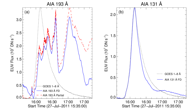
Figure 4.: Light curves of AIA images in (a) 193 Å and (b) 131 Å channels for a M1.1 flare in comparison with the GOES soft X-ray time variations. In 193 Å, there are variations that do not track the GOES, although a good match is seen in 131 Å. Even if the field of view is restricted to a sub-field around the flare (see the line in red) as opposed to full-disk (FD), the variations observed in 193 Å remain, suggestive of increase of low-temperature material in the flare that is not observed by GOES. lc˙193˙131

For less intense flares, there are more complications in the 193 Å data due primarily to the flux of cool plasma that contributes to the main response around 1.5 MK. In full-disk 193 Å images, the flare contribution is typically only $\approx$10% of the total flux in a X1 flare, meaning that it can be only 0.5% for a C5 flare. Therefore background subtraction produces significant uncertainties, especially for less intense events. Variations of coronal plasma outside the flare region may be excluded by analyzing the fluxes in a small area surrounding the flare. However, this does not always work for flares less intense than, for example, the GOES M3 – M4 level ($F_{1-8}$ = (3 – 4)$\times$10^-5 W m^-2). Figure 4(a) shows that the light curves are not well correlated between the GOES and 193 Å  and that this does not change substantially if we use the flux within a sub-field (300$\hbox{${}^{\prime\prime}$}\times$300^′′). Furthermore, we could not find a sub-field in which the first peak that corresponds to the GOES peak is higher than the second peak around 17:03 UT. This example thus indicates that some flares can have a higher emission measure at 1.5 MK relative to 20 MK than found by Dere and Cook Dere and Cook (1979). For this M1.1 flare (SOL2011-07-27T16:07), the 131 Å flux is still well-correlated with the GOES (Figure 4(b)). One of the reasons that smaller flares correlate better with the 131 Å than with the 193 Å may be that they are cooler, and thus reach temperatures of Fe xxi but not those of Fe xxiv.

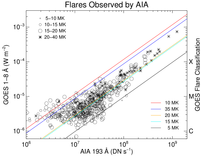
Figure 5.: Scatter plot of the GOES 1 – 8 Å and AIA 193 Å background-subtracted fluxes of 540 flares. In each flare, the GOES-AIA pair is made around the X-ray peak time. The five lines show how the relation of the GOES and AIA fluxes depends on the temperature of the flare. The order reflects the AIA response relative to the GOES response (see Figure 2(b)). The size of the symbols represents the flare temperature as determined by the GOES 0.5 – 4 Å and 1 – 8 Å ratio. aia˙xrs

Coronal dimming can also play a major role in less intense flares than those shown in Figure 3. Out of the 609 flares above C3 and observed in AIA’s normal mode, 69 flares, mostly C-class, show less 193 Å flux at the GOES peak than during the preflare interval. The most intense flare in this categoy is M2.5. The frequency of a smaller flux at the flare peak is not not much different if we include only a small area around the flare because of deeper dimming closer to the flare.

Cooling plasma from previous flares can contribute to the main response of the 193 Å channel, making it difficult to determine the background level. This is especially true when the increase of flux due to the flare is only a few percent of less. Therefore, flares that occur one after another can pose a serious problem for comparing EUV and X-ray fluxes.

In Figure 5, we show a scatter plot of the AIA 193 Å and GOES XRS 1 – 8 Å fluxes around the GOES peak times. Both fluxes reflect pre-flare background subtraction. This includes all the 540 flares that have positive 193 Å fluxes. The time difference between the AIA and GOES fluxes is only up to the three-second sampling rate of the latter. Different symbols are used to indicate the GOES XRS channel ratio temperature White et al. (2005). Pearson’s correlation coefficient for the fluxes in the logarithmic scales is 0.81 for the entire population and 0.92 for the 51 flares above M3. The lines represent the expected relations between the GOES and AIA fluxes for flares characterized by single temperatures (see Figure 2(b)). Most points above the M3 level fall between $T=$15 MK and $T=$35 MK lines. The GOES channel ratio temperature is generally above 15 MK for these flares. The scatter in this plot could be made smaller first by limiting the area and then by conducting pixel-to-pixel differential measure analyses and extracting only those pixels that contain hot plasma to be observed by GOES. It is beyond the scope of this article, although such an effort could be instructive.

4 GOES EUVI Relation

GOES-EUVI

Figure 6.: The distribution of the flare rise time from the NOAA flare list. rise˙time

Now we apply the same analysis on EUVI 195 Å data. The most significant difference of these images from AIA images is that they are taken much less frequently, typically once every five minutes. This may mean a poorer correlation with the GOES XRS flux because the next image after the flare onset can be after the flare peak, by which time the excess in EUV flux may already start. In Figure 6, for all the flares included in the NOAA flare list, we plot the time difference between the soft X-ray peak and onset as a function of the X-ray peak flux. Most flares above the M4 level have the rise time longer than 4 minutes, so it is likely that for most intense flares the rising phase is included where we expect a good correlation between GOES and EUVI 195 Å. There were intense flares in 2007 up to M8 Aschwanden et al. (2009); Nitta et al. (2013), but we cannot include them because their rise times are typically less than ten minutes, and 195 Å images were taken only once every ten minutes. Until August 2009, EUVI’s “primary wavelength” was 171 Å.

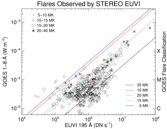
Figure 7.: Scatter plot of the GOES 1 – 8 Å and EUVI 195 Å fluxes of $\approx$450 flares. Only those flares observed by AIA and not occulted from STEREO’s view are plotted. The same format as Figure 5. The order of the lines representing five temperatures reflects the EUVI response relative to the GOES response (see Figure 2(b)).euvi˙xrs

From the same set of flares that are plotted in Figure 5, we select only those that were observed on disk by one or both STEREO spacecraft. This is achieved within SolarSoft Freeland and Handy (1998) by combining the flare locations on flares that come from the Heliophysics Event Registry Hurlburt et al. (2012) with the STEREO orbital information. We also drop those flares in which the time difference of the EUVI image from the GOES peak time is more than five minutes. This leaves a total of 450 flares with Ahead and Behind combined. No distinction is made between the EUVI flux from Ahead and Behind, since the response of the 195 Å channel to 10 MK differs by only $\approx$4%. For the flares that were observed without occultation by EUVI on both spacecraft, we usually use data from Ahead. We correct the EUVI flux as if the STEREO were located at the same distance as the Earth from the Sun.

Figure 7 is a plot of the observed GOES and full-disk EUVI fluxes. Pearson’s correlation coefficient is 0.67 for the entire population, but as high as 0.94 for the 32 flares above M3. One unresolved issue, however, is that most points representing intense flares lie around or below the $T=$15 MK line (e.g., the rightmost point, which is the X6.9 flare of SOL2011-08-09T08:05 Asai et al. (2012)), suggesting the need for fine tuning of the EUVI absolute flux calibration.

Figure 8.: The ratio of the observed GOES flux with the expected flux from EUVI 195 Å flux assuming an isothermal plasma of 20 MK.euvi˙exp˙scatter

Irrespective of the absolute calibration, we can now use the points of intense flares to estimate the GOES peak X-ray flux. In Figure 8 we show how much the scatter is from what is expected by assuming that flares have a single temperature of 20 MK. Here the error bars reflect a crude estimate of the uncertainty of the EUVI flux, where it increases from 3% at $F_{\rm{EUVI(195)}}=10^{8}$ to 50% at $F_{\rm{EUVI(195)}}=10^{4}$. This is based on an inspection of temporal variations of the EUVI flux in comparison with the XRS flux for all the events included here.

Figure 8 suggests that we can determine the GOES peak X-ray flux for flares more intense than M4 to within the factor of three. The best fit we find is

$$F_{\rm{GOES}}=1.39\cdot 10^{-11}F_{\rm{EUVI(195})}$$ (1)

The uncertainty is larger for less intense flares as is clear from the larger scatter. Nevertheless, it is not much larger than an order of magnitude, so for convenience we will put the range of 0.5 – 1.5 of Equation (1) for flares with $F_{\rm{EUVI(195)}}>4\cdot 10^{6}$ DN s^-1 and 0.3 – 3 for flares with $F_{\rm{EUVI(195)}}\lesssim 4\cdot 10^{6}$ DN s^-1.

5 Major Events on the Farside

Examples

We have surveyed the mission-long EUVI archive and found a number of candidates of X-class flares. Table 1 lists them with their locations and estimated ranges of the GOES peak X-ray flux. It also includes a few less intense flares that have been discussed largely in the context of multi-spacecraft observations of solar energetic particle (SEP) events Dresing et al. (2012); Rouillard et al. (2012); Mewaldt et al. (2012). It turns out that these events (17 January 2010, 21 March 2011, and 3 November 2011) are not particularly intense in the GOES scale. But at least the first two events stand out in terms of one of the attributes of the CME, namely an EUV wave Veronig et al. (2010); Rouillard et al. (2012).

We have a few notes concerning the list in Table 1. First, the frequency of candidates of X-class flares behind the limb mimics that of the X-class flares actually observed on the visible side. Single active regions may produce multiple X-class flares over a wide range of longitude. Although we had to wait until 15 February 2011 for the first X-class flare in solar cycle 24, the flare on 31 August 2010 was probably the first one.

Table 1.: List of major events since 2010 that come from regions $>$30^∘ behind the limb. These are either candidates of X-class flares or multi-spacecraft SEP events. The four events that are shown in Figure 9 are marked with asterisks. T-simple

Date	Time	A or B	Location	Est. $F_{\rm{GOES}}$	Range	Refs
2010/01/17	03:55:40	B	S25 E128	6.4$\cdot$10-5	M3.4 – M9.6	1, 2
2010/08/31	20:55:53	A	S22 W146	1.7$\cdot$10-4	M8.4 – X2.5
2010/09/01	21:50:53	A	S22 W162	1.1$\cdot$10-4	M5.4 – X1.6
2011/03/21	02:10:49	A	N20 W128	3.1$\cdot$10-5	M1.3 – X1.3	3
2011/06/04	07:05:58	A	N15 W140	1.0$\cdot$10-4	M5.2 – X1.6
2011/06/04 *	21:50:58	A	N17 W148	8.1$\cdot$10-4	X4.0 – X12
2011/10/23	23:15:44	A	N19 W151	1.1$\cdot$10-4	X5.3 – X1.6
2011/11/03 *	22:40:44	B	N08 E156	9.4$\cdot$10-5	M4.7 – X1.4	4
2012/03/26	22:16:02	B	N18 E123	1.6$\cdot$10-4	M8.2 – X2.5
2012/04/29	12:45:53	B, A	N12 E163	1.7$\cdot$10-4	M8.3 – X2.5
2012/07/23 *	02:30:56	A	S15 W133	1.5$\cdot$10-4	M8.2 – X2.5
2012/08/21	20:10:54	B, A	S22 E158	1.4$\cdot$10-4	M6.8 – X2.0
2012/09/11	07:55:50	B, A	S22 E178	2.6$\cdot$10-4	X1.3 – X3.9
2012/09/19	11:15:49	B, A	S15 E171	1.8$\cdot$10-4	M9.1 – X2.7
2012/09/20 *	15:00:48	B, A	S15 E153	1.2$\cdot$10-3	X5.8 – X18
2012/09/22	03:05:48	B	S15 E134	1.7$\cdot$10-4	M8.4 – X2.5

References: 1. Veronig et al. (2010), 2. Dresing et al. (2012), 3. Rouillard et al. (2012), 4. Mewaldt et al. (2012)

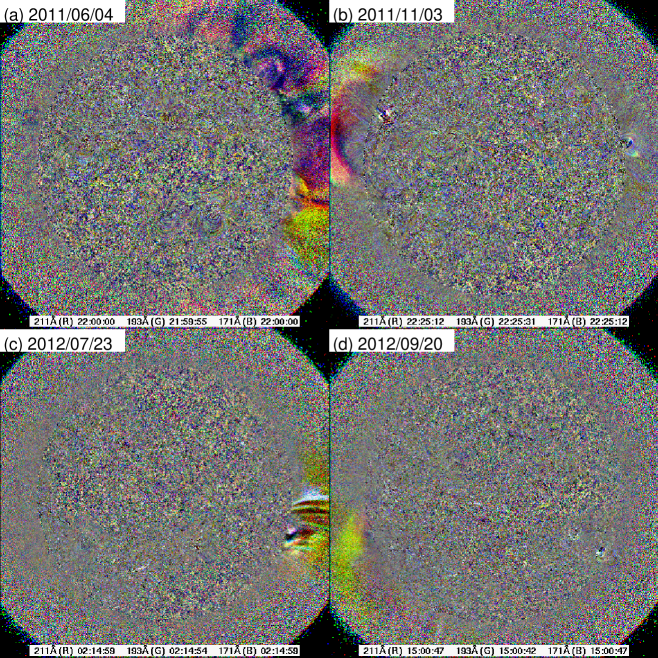
Figure 9.: Running ratio images of four events that occurred far behind the limb (see Table 1 for their locations), and were observed directly by AIA because of high cadence and sensitivity. tri˙color

EUVI data of these behind-the-limb flares (from Earth view) show a varied degree of association with CMEs. While some are confined and not associated with a major CME in white-light coronagraph data, others are highly eruptive, also accompanying extended dimming. Note that dimming is usually observed only after a sharp increase of flux, indicating that the peak flux is well captured. Some of the highly eruptive events, despite deep occultation by the limb, emerge in AIA images either as an eruption itself or in the form of waves or propagating fronts. Figure 9 gives snapshots from the tri-color running ratio movies that are accessible at http://aia.lmsal.com/occulted˙events. We also point out that the event on 23 July 2012 is more eruptive than that on 20 September 2012, which is probably the most intense flare in solar cycle 24 as of the end of 2012.

6 Summary and Discussion

S-Discussion

We have correlated GOES X-ray and EUV (195 Å) fluxes of 450 flares as observed by STEREO, and found an empirical relation, which lets us estimate the GOES peak X-ray flux of intense events, whose X-ray emission is occulted by the limb. There are more than a dozen candidates of X-class flares as shown in Table 1. Many of the events included here to obtain the EUVI-XRS flux relation have impulsive time profiles, and in such events it is possible that we may underestimate the soft X-ray flux by missing the real peak because of the EUVI five-minute cadence limitation.

Using AIA observations we study the origins and extents of uncertainties in the estimation of the peak GOES X-ray flux from EUV data. The main difficulty lies in the fact that the Fe xxiv line represents only a small secondary response peak in the 195 Å (193 Å) channel. The main response peak not only picks up cooling or heating plasma from the present and previous flares in the 1 – 2 MK range but also shows decrease because of coronal dimming when the flare is associated with a CME. It appears that the effect of coronal dimming is not substantial until the soft X-ray peak in flares above M3 or so, but it can be significant in less intense flares. In extreme cases, the 193 Å flux is found to decrease in the rising phase of the flare. The primary response of AIA’s 193 Å and EUVI’s 195 Å channels is around 1.5 MK, and in order to correlate the fluxes in these channels with the GOES flux, we should in principle extract those pixels that contain $\mathrel{\hbox{\hbox to0.0pt{\hbox{\lower 4.0pt\hbox{$\sim$}}\hss}\hbox{$>$}}}$10 MK plasma, by conducting differential emission measure analysis. One caveat is that one needs to monitor full-disk images for sympathetic flaring at a remote region, which may also contribute to the spatially-integrated GOES flux.

Other related issues include the absolute calibration of the involved instruments, including the GOES XRS. We used calibration data for the XRS on GOES-14, but most flares analyzed in this work were observed by the XRS on GOES-15, whose response data have not been available (S. White, personal communication, 2012). Also needed is a fine tuning as to the absolute calibration of EUVI and AIA. Apart from the calibration of the instruments, we have not considered the possible effect of non-thermal flare emission (especially on GOES) and ionization equilibrium of hot plasma.

Lastly, we may ask how significant the GOES X-ray flare classification is for the interpretation of energetic events. We have conventionally and conveniently used the GOES X-ray class as if it represents the magnitude of the flare. However, it is argued that the energy radiated in soft X-rays is only a small fraction of the total energy released in flares (e.g., Kretzschmar et al., 2010). For the total energy budget, we should include presumably larger energy that goes into Sun’s lower atmosphere. The fact that even C-class flares produce white-light emission (e.g., Matthews et al., 2003) indicates that the X-ray flux may not be correlated with the total energy. Here we consider the GOES X-ray flux to be still an important reference, however, thanks partly to its existence for more than three solar cycles. As demonstrated by the recent work of Ryan et al. Ryan et al. (2012), the GOES XRS measurement is useful for collectively deriving flare plasma parameters, even though it is also possible that we may find in SDO data a better parameter more intimately correlated with the total energy that includes energy flow both into the heliosphere and lower atmosphere.

Acknowledgements

This work has been supported by the NASA STEREO mission under NRL Contract No. N00173-02-C-2035, and by the AIA contract NNG04EA00C to LMSAL. We are greateful to the referee for valuable comments that clarified the motivations of this work.

References

- Aschwanden et al. (2009) Aschwanden, M.J., Wuelser, J.-P., Nitta, N.V., Lemen, J.R. : 2009, Sol. Phys. 256, 3. doi: 10.1007/s11207-009-9347-4
- Asai et al. (2012) Asai, A., Ishii, T.T., Isobe, H., Kitai, R., Ichimoto, K., UeNo, S., Nagata, S., Morita, S., Nishida, K., Shiota, D., Oi, A., Akioka, M., Shibata, K.: 2012, ApJ 745, L18. doi: 10.1088/2041-8205/745/2/L18
- Battaglia, Grigis, and Benz (2005) Battaglia, M., Grigis, P.C., Benz, A.O.: 2005, A&A 439, 737. doi: 10.1051/0004-6361:20053027
- Boerner et al. (2012) Boerner, P., Edwards, C., Lemen, J., Rausch, A. Schrijver, C., Shine, R., Shing, L. Stern, R., Tarbell, T., Title, A., Wolfson, C. J., Soufli, R., Spiller, E., Gullikson, E., McKenzie, D., Windt, D., Golub, L. Podgorski, W., Testa, P., Weber, M.: 2012, Sol. Phys. 275, 41. doi: 10.1007/s11207-011-9804-8
- Delaboudinière et al. (1995) Delaboudinière, J.-P., Artzner, G.E., Brunaud, J., Gabriel, A.H., Hochedez, J.F., Millier, F., Song, X.Y., Au, B., Dere, K.P., Howard, R.A., Kreplin, R., Michels, D.J., Moses, J.D., Defise, J.M., Jamar, C., Rochus, P., Chauvineau, J.P., Marioge, J.P., Catura, R.C., Lemen, J.R., Shing, L., Stern, R.A., Gurman, J.B., Neupert, W.M., Maucherat, A., Clette, F., Cugnon, P., van Dessel, E.L.: 1995, Sol. Phys. 162, 291. doi: 10.1007/BF00733432
- Dere and Cook (1979) Dere, K.P., Cook, J.W.: 1979, ApJ 229, 772. doi:10.1086/157013
- Dere, et al. (1997) Dere, K.P., Landi, E., Mason, H.E., Monsignori Fossi, B.C., Young, P.R.: 1997, A&AS 125, 149. doi: 10.1051/aas:1997368
- Dresing et al. (2012) Dresing, N., Gómez-Herrero, R., Klassen, A., Heber, B., Kartavukh, Y., Dröge, W.: 2012, Sol. Phys. 281, 281. doi: 10.1007/s11207-012-0049-y
- Feldman et al. (1996) Feldman, U., Doscheck, G.A., Behring, W.E., Phillips, K.J.H.: 1996, ApJ 460, 1034. doi: 10.1086/177030
- Fletcher et al. (2011) Fletcher, L., Dennis, B.R., Hudson, H.S., Krucker, S., Phillips, K., Veronig, A., Battaglia, M., Bone, L., Caspi, A., Chen, Q., Gallagher, P., Grigis, P.T., Ji, H., Liu, W., Milligan, R.O., Temmer, M.: 2011, Space Sci. Rev. 159, 19. doi: 10.1007/s11214-010-9701-8
- Freeland and Handy (1998) Freeland, S.L., Handy, B.N.: 1998, Solar Phys. 182, 497. doi: 10.1023/A:1005038224881
- Howard et al. (2008) Howard, R.A., Moses, J.D., Vourlidas, A., Newmark, J.S., Socker, D.G., Plunkett, S.P., Korendyke, C.M., Cook, J.W., Hurley, A., Davila, J.M., Thompson, W.T., St Cyr, O.C., Mentzell, E., Mehalick,K., Lemen, J.R., Wuelser, J.-P., Duncan, D.W., Tarbell, T.D., Wolfson, C.J., Moore, A., Harrison, R.A., Waltham, N.R., Lang, J., Davis, C.J., Eyles, C.J., Mapson-Menard, H., Simnett, G.M., Halain, J.P., Defise, J.M., Mazy, E., Rochus, P., Mercier, R., Ravet, M.F., Delmotte, F., Auchère, F., Delaboudinière, J. P., Bothmer, V., Deutsch, W., Wang, D., Rich, N., Cooper, S., Stephens, V., Maahs, G., Baugh, R., McMullin, D., Carter, T.: 2008, Space Sci. Rev. 136, 67. doi: 10.1007/s11214-008-9341-4
- Hurlburt et al. (2012) Hurlburt, N., Cheung, M., Schrijver, C., Chang, L., Freeland, S., Green, S., Heck, C., Jaffey, A., Kobashi, A., Schiff, D., Serafin, J., Seguin, R., Slater, G., Somani, A., Rimmons, R.: 2012, Sol. Phys. 275, 67. doi: 10.1007/s11207-010-9624-2
- Kaiser et al. (2008) Kaiser, M.L., Kucera, T.A., Davila, J.M., St.Cyr, O.C., Guhathakurta, M., Christian, E.: 2008, Space Sci. Rev. 136, 5. doi: 10.1007/s11214-007-9277-0
- Kretzschmar et al. (2010) Kretzschmar, M., Dudok de Wit, T., Schumutz, W., Mekaoui, S., Hochedez, J.-F., Dewitte, S.: 2010, Nature Physics 6, 690. doi: 10.1038/nphys1741
- LaBonte, Georgoulis, and Rust (2007) LaBonte, B.J., Georgoulis, M.K., Rust, D.M.: 2007, ApJ 671, 955. doi: 10.1086/522682
- Landi et al. (2012) Landi, E., Del Zanna, G., Young, P.R. Dere, K.P., Mason, H.E.: 2012, ApJ 744, 99. doi: 10.1088/0004-637X/744/2/99
- Lemen et al. (2012) Lemen, J.R., Title, A.M., Akin, D.J., Boerner, P.F., Chou, C., Drake, J.F., Duncan, D.W., Edwards, C.G., Friedlaender, F.M., Heyman, G.F., Hurlburt, N.E., Katz, N.L., Kushner, G.D., Levay, M., Lindgren, R. W., Mathur, D. P., McFeaters, E.L., Mitchell, S., Rehse, R.A., Schrijver, C.J., Springer, L.A., Stern, R.A., Tarbell, T.D., Wuelser, J.-P., Wolfson, C.J., Yanari, C., Bookbinder, J.A., Cheimets, P.N., Caldwell, D., DeLuca, E.E., Gates, R., Golub, L., Park, S., Podgorski, W.A., Bush, R.I., Scherrer, P.H., Gummin, M.A., Smith, P., Auker, G., Jerram, P., Pool, P., Soufli, R., Windt, D.L., Beardsley, S., Clapp, M., Lang, J., Waltham, N.: 2012, Solar Phys. 275, 17. doi: 10.1007/s11207-011-9776-8
- Matthews et al. (2003) Matthews, S.A., van Driel-Gesztelyi, L., Hudson, H.S., Nitta, N.V.: 2003, A&A 409, 1107. doi: 10.1051/0004-6361:20031187
- Mewaldt et al. (2012) Mewaldt, R.A., Cohen, C.M.S., Mason, G.M., von Rosenvinge, T.T., Leske, R.A., Luhmann, J.G., Odstrcil, D., Vourlidas, A.: 2012, In: Solar Wind 13 Conference Proceedings.
- Nitta et al. (2013) Nitta, N.V., Aschwanden, M.J., Freeland, S.L., Lemen, J.R., Wuelser, J.-P., Zarro, D.M.: 2013, Sol. Phys. submitted.
- Pesnell, Thompson, and Chamberlin (2012) Pesnell, W.D., Thompson, B.J., Chamberlin, P.C.: 2012, Sol. Phys. 275, 3. doi: 10.1007/s11207-011-9841-3
- Rouillard et al. (2012) Rouillard, A.P., Sheeley, N.R., Jr., Tylka, A., Vourlidas, A., Ng, C.K., Rakowski, C., Cohen, C.M.S., Mewaldt, R.A., Mason, G.M., Reames, D., Savani, N.P., St. Cyr, O.C., Szabo, A.: 2012, ApJ 752, 44. doi: 10.1088/0004-637X/752/1/44
- Ryan et al. (2012) Ryan, D.F., Milligan, R.O., Gallagher, P.T., Dennis, B.R., Tolbert, A.K., Schwartz, R.A., Young, C.A.: 2012, ApJS 202, 11. doi: 10.1088/0067-0049/202/2/11
- Schrijver et al. (2011) Schrijver, C.J., Aulanier, G., Title, A.M., Pariat, E., Delannée: 2011, ApJ 738, 167. doi: 10.1088/0004-637X/738/2/167
- Sudol and Harvey (2005) Sudol, J.J., Harvey, J.W.: 2005, ApJ 635, 647. doi: 10.1086/497361
- Veronig et al. (2010) Veronig, A.M., Muhr, N., Kienreich, I.W., Temmer, M., Vršnak, B.: 2010, ApJ 716, L57. doi: 10.1088/2041-8205/716/1/L57
- White et al. (2005) White, S.M., Thomas, R.J., Schwartz, R.A.: 2005, Sol. Phys. 227, 231. doi: 10.1007/s11207-005-2445-z
- Wuelser et al. (2004) Wuelser, J.-P., Lemen, J.R., Tarbell, T.D., Wolfson, C.J., Cannon, J.C., Carpenter, B.A., Duncan, D.W., Gradwohl, G.S., Meyer, S.B., Moore, A.S., Navarro, R.L., Pearson, J.D., Rossi, G.R., Springer, L.A., Howard, R.A., Moses, J.D., Newmark, J.S., Delaboudinière, J.-P., Artzner, G.E., Auchère, F., Bougnet, M., Bouyries, P., Bridou, F., Clotaire, J.-Y., Colas, G., Delmotte, F., Jerome, A., Lamare, M., Mercier, R., Mullot, M., Ravet, M.-F., Song, X., Bothmer, V., Deutsch, W.: 2004, In: Fineschi, S., Gummin, M.A. (eds.), Telescopes and Instrumentation for Solar Astrophysics, Proc. SPIE 5171, 111. doi: 10.1117/12.506877