On the Tidal Dissipation of Obliquity

Abstract

We investigate tidal dissipation of obliquity in hot Jupiters. Assuming an initial random orientation of obliquity and parameters relevant to the observed population, the obliquity of hot Jupiters does not evolve to purely aligned systems. In fact, the obliquity evolves to either prograde, retrograde or 90^o orbits where the torque due to tidal perturbations vanishes. This distribution is incompatible with observations which show that hot jupiters around cool stars are generally aligned. This calls into question the viability of tidal dissipation as the mechanism for obliquity alignment of hot Jupiters around cool stars.

1. Introduction

Hot Jupiters (with masses comparable to that of Jupiter and orbital periods less than a week or so) are found around 1-2 % of solar type stars. A widely adopted scenario for their origin is that these planets formed at several AU from their host stars and underwent inward migration due to tidal interaction with their natal disks (Lin et al., 1996). Another class of dynamical models assumes the hot Jupiters were relocated to close proximity to their host stars through close encounters between planets, secular chaos, or Kozai resonance with companion stars (Rasio & Ford, 1996; Wu & Murray, 2003; Fabrycky & Tremaine, 2007; Wu & Lithwick, 2011; Naoz et al., 2011).

New observations are continually testing and constraining these theories. To date the obliquity between planets and their host stars have been measured using the Rossiter-McLaughlin effect in more than 50 systems. Several hot Jupiters have been observed to have high obliquity, $\Theta$ (including retrograde orbits in which $\Theta>\pi/2$), while many show alignment. In general, hot Jupiters around cool stars with effective temperature $T_{\ast}<6,250$K, tend to be aligned, while those around hot stars, $T_{\ast}>6,250$K, appear to be misaligned (Winn et al., 2010). In order to account for this dichotomy, Winn et al. (2010) and subsequently, Albrecht et al. (2012) have suggested that 1) all hot Jupiters were relocated to close proximity to their host stars by one of the dynamical processes described above, resulting in a random distribution of obliquity, 2) the obliquities of those planets around cool stars are damped by efficient tidal dissipation in the convective envelopes of these cool stars and 3) the obliquities of those planets around hot stars, with radiative envelopes, reflects that of the initial random obliquity distribution because tidal dissipation in these systems is inefficient.

Quantitatively, Albrecht et al. (2012) evaluated the magnitude of the tidal dissipation time scale in stars with convective envelopes, $\tau_{CE}$, and those with radiative envelopes, $\tau_{RA}$ using models of equilibrium tides for convective solar-type stars and dynamical tides for radiative, intermediate-mass stars (Zahn, 1977). They showed a correlation between the magnitude of misalignment, $\Theta$, and the dissipation timescales.

Despite this suggestive evidence, there are large uncertainties in the equilibrium-tide model that Albrecht et al. (2012) have adopted, mostly due to a controversial prescription for turbulent dissipation of the tides (Goldreich & Nicholson, 1989; Terquem et al., 1998; Ogilvie & Lin, 2007; Barker & Ogilvie, 2010). Using Zahn’s model, Albrecht et al. (2012) calculate that the magnitudes of $\tau_{CE}/\tau_{\ast}$ and $\tau_{RA}/\tau_{\ast}$ vary by several orders of magnitude (see their Figures 24 & 25). The relatively small value of $\tau_{CE}/\tau_{\ast}$ obtained for many of the aligned hot Jupiters around solar type stars pose a challenge to their retention against substantial orbital decay, unless the time scale for obliquity damping is substantially smaller than that for orbital decay.

In a thorough theoretical analysis, Lai (2012) showed that the timescale for obliquity damping could be substantially different from that of orbital decay. He identified a component of the tidal torque which affects the obliquity alignment but not the orbital decay. He showed that, for the forcing frequency of this particular component of the tidal perturbation, inertial waves may be excited to provide a dynamical tidal response which could lead to much more efficient energy dissipation and hence, shorter dissipation timescales. Therefore, the Lai (2012) theory appears to provide a potential mechanism to account for hot Jupiters whose obliquity has been damped in absence of substantial orbital decay.

In §2, we briefly recapitulate Lai’s theory and in §3 show that the orbital decay paradox can only be resolved if the timescale for obliquity evolution is much smaller than that for semi-major axis decay. In the limit of negligible orbital decay, we show in §3, that tidal dissipation does not lead to obliquity alignment. Both of these effects have been clearly stated by Lai (2012). Our contribution is to provide the results of numerical integration for various limiting cases and compare them with the observational data. We discuss the implications of our results in §4.

2. Semi major axis decay and obliquity alignment

We first briefly recapitulate the theory of equilibrium and dynamical tides raised by hot Jupiters on their host stars.

2.1. Components of planets’ tidal perturbation on their spinning host stars

The tidal potential $U({\bf r},t)$ imposed by a planet with mass $M_{p}$, with a circular orbit and an orbital angular frequency ${\Omega_{p}}$ on a star with a mass $M_{\ast}$ and a uniform spin with angular frequency ${\Omega_{\ast}}$ can be approximated to the lowest order in terms of spherical harmonics in a frame centered on the star with the z-axis parallel to the stellar spin such that

$$U({\bf r},t)=-\sum_{mm^{\prime}}U_{mm^{\prime}}(M_{p},\Theta)r^{2}Y_{2m}(\theta,\phi){\rm exp}\left(-im^{\prime}\Omega_{p}t\right)$$ (1)

where the obliquity $\Theta$ is the angle between the stellar spin S and planet’s orbital angular momentum vector L, whereas the magnitudes are given by $S=I\Omega_{\ast}$ and $L=M_{p}a^{2}\Omega_{p}$, $I=kM_{\ast}R_{\ast}^{2}$, where $R_{\ast}$ is the stellar radius, $k(\simeq 0.1)$ and $I$ is the moment of inertia. In a frame co-rotating with the stellar spin, the forcing frequency is $\omega_{mm^{\prime}}=m^{\prime}\Omega_{p}-m\Omega_{\ast}$ with seven components contributing to obliquity evolution (Barker & Ogilvie, 2009).

Lai (2012) pointed out that it is possible for some components of the planets’ tidal perturbing potential to have sufficiently small $\omega_{mm^{\prime}}<2\Omega_{\ast}$ to allow the corilois effect to provide the necessary restoring force for the excitation of inertial waves (Greenspan, 1968). In cool stars these waves lead to dynamical tides (Ogilvie & Lin, 2007). For some forcing frequencies, the inertial waves may converge onto attractors and dissipate more efficiently (Ogilvie & Lin, 2004). Lai (2012) showed that in the limit of small $\Omega_{\ast}(<\Omega_{p})$, the only component of the perturbing potential with sufficiently small $\omega_{mm^{\prime}}$ is that associated with $(m,m^{\prime})=(1,0)$. For this component, tidal dissipation can lead to a shorter dissipation timescale and obliquity evolution without significant orbital decay. For more rapidly spinning stars (with $\Omega_{\ast}>\Omega_{p}/2$), it is possible to excite other components of the tidal response which would lead to both obliquity evolution and orbital decay.

2.2. Evolutionary equations

We first consider the possibility that the dissipation timescale, $t_{mm^{\prime}}$ is indentical for all $(m,m^{\prime})$ components. In this case, dissipation of the equilibrium tide leads to

$${{\dot{a}}_{e}\over a}=-{1\over\tau_{e}}\left(1-{\Omega_{\ast}\over\Omega_{p}}{\rm cos}\Theta\right)$$ (2)

$${{\dot{\Omega}}_{\ast e}\over\Omega_{\ast}}={1\over\tau_{e}}\left({L\over 2S}\right)\left[{\rm cos}\Theta-\left({\Omega_{\ast}\over 2\Omega_{p}}\right)(1+{\rm cos}^{2}\Theta)\right]$$ (3)

$${\dot{\Theta}}_{e}=-{1\over\tau_{e}}\left({L\over 2S}\right){\rm sin}\Theta\left[1-\left({\Omega_{\ast}\over 2\Omega_{p}}\right)\left({\rm cos}\Theta-{S\over L}\right)\right]$$ (4)

where $\tau_{e}=(Q_{a}/3k_{2})(M_{\ast}/M_{p})(a/R_{\ast})^{5}(P/2\pi)$ is the characteristic orbital evolution time scale, $k_{2}$ is the Love number, and $Q_{a}$ is the highly uncertain quality factor. In addition to turbulent dissipation of equilibrium tides, $Q_{a}$ may also include contributions from the dissipation of internal gravity and inertial waves in solar type stars (Ogilvie & Lin, 2007). For rapidly spinning stars, the dynamical response associated with the inertial waves may lead to the evolution of $a$ and $\Theta$ on similar time scales.

However, for slowly spinning stars (with $\Omega_{\ast}<\Omega_{p}/2$), only the forcing frequency associated with the $(m,m^{\prime})=(1,0)$ component can excite the inertial modes, leading to a dynamical response, and relatively short timescales $\tau_{10}(<<\tau_{e})$. The dynamical tide’s contribution associated with the (1,0) component of the torque leads to rates of change of $a$, $\Omega_{\ast}$, and $\Theta$ such that

$${{\dot{a}}\over a}={{\dot{a}}_{e}\over a},$$ (5)

$${{\dot{\Omega}}_{\ast}\over\Omega_{\ast}}=\left({{\dot{\Omega}}_{\ast}\over\Omega_{\ast}}\right)_{e}+\left({{\dot{\Omega}}_{\ast}\over\Omega_{\ast}}\right)_{10}+\left({{\dot{\Omega}}_{\ast}\over\Omega_{\ast}}\right)_{10,e},$$ (6)

$${\dot{\Theta}}=\left({\dot{\Theta}}\right)_{e}+\left({\dot{\Theta}}\right)_{10}-\left({\dot{\Theta}}\right)_{10,e},$$ (7)

where

$$\left({{\dot{\Omega}}_{\ast}\over\Omega_{\ast}}\right)_{10}=-{1\over\tau_{10}}\left({\rm sin}\Theta{\rm cos}\Theta\right)^{2}$$ (8)

$$\left({\dot{\Theta}}\right)_{10}=-{1\over\tau_{10}}{\rm sin}\Theta{\rm cos}^{2}\Theta\left({\rm cos\Theta+{S\over L}}\right),$$ (9)

$${{\dot{\Omega}}_{\ast,10,eq}\over{\dot{\Omega}}_{\ast,10}}={{\dot{\Theta}_{10,eq}\over{\dot{\Theta}}_{10}}={Q_{10}\over Q_{a}}{k_{2}\over k_{10}}},$$ (10)

$$\tau_{10}=\left({4Q_{10}\over 3k_{10}}\right)\left({M_{\ast}\over M_{p}}\right)\left({a\over R_{\ast}}\right)^{5}\left({S\over L}\right)\left({P\over 2\pi}\right)$$ (11)

such that $\tau_{10}/\tau_{e}\sim(Q_{10}/Q_{a})(k_{2}/k_{10})(S/L)$. Lai (2012) pointed out that since the $(m,m^{\prime})=(1,0)$ component does not contribute to $\dot{a}$, obliquity alignment can occur, in principle, prior to any significant orbital decay if $\tau_{10}<<\tau_{e}$.

3. Computational results

3.1. Evolution of Semi-Major axis and Obliquity due to Equilibrium Tide

Here we show that the obliquity alignment due to the equilibrium tide is accompanined by substantial orbital evolution. We first neglect any extra contribution from the $(m,m^{\prime})=(1,0)$ component by numerically integrating Equations (2-4), with a fourth order Runge-Kutta scheme, for an inital value of $\Theta_{o}=45^{o}$. If we fix $k(R_{\ast}/a_{o})^{2}(M_{\ast}/M_{p})=1$, we have a set of solutions which depend only on the initial value of S/L. The solutions to these integrations are shown in Figure 1. In that figure, black lines represent the evolution of $a(t)/a_{o}$, red lines represent the evolution of $\Theta$ and the blue lines represent the evolution of the equilibrium timescale (which varies as $a^{-13/2}$) all as a function of time, in units of the (initial) equilibrium timescale.

Concentrating first on the slow rotators (S/L $<$1) we see two important features. First, in order to have significant obliquity damping the semi-major axis is reduced substantially. Given that we set our initial ratio ($R_{\ast}/a_{o}$) to 0.1 any reduction of $a$ below this value implies the planet has fallen into the star. We see that this occurs at approximately 2.5 T_eq0, a time when there is still non-negligible obliquity. Another way to look at this is to consider the time when the obliquity is damped to half its original value of $\pi$/4, at this time the equilibrium timescale has been reduced by nearly five orders of magnitude. One might hypothesize that we have caught the aligned hot Jupiters in their last gasp on their death march to infall in which their obliquity has been reduced to zero but their orbits have not been completely exhausted. However, the rapid decay of the equilibrium timescale coincident with this evolution is not consistent with the large population of aligned, yet surviving, systems that have been observed. In summary, even modest amounts of obliquity damping are concurrent with significant orbital decay and a rapidly decreasing timescale over which that orbital decay will occur. Similarly, for fast rotators modest obliquity damping is accompanied by significant orbital expansion. Therefore, in order to accomodate any substantial obliquity evolution the planet would have to have started its orbit virtually inside the star, an impossible scenario.

Therefore, for both slow and fast rotators it is impossible to get any substantial obliquity evolution without either 1) the planet falling into the star (slow rotators) or 2) the planet starting its orbital evolution inside the star (fast rotators). This long recognized problem leads to the conclusion that significant obliquity damping can only occur if the dynamical tide is considered and the timescale for obliquity alignment, $\tau_{10}$ is substantially less than that for orbital decay/expansion, $\tau_{eq}$.

3.2. Population synthesis of obliquity evolution due to dynamical tides

The model of Albrecht et al. (2012) assumes that hot jupiters arrived at their current, close positions with a random distribution of obliquities as a result of one of the dynamical processes listed in §1. To mimic this scenario we start from a random distribution of obliquities and integrate Equation (7), assuming a constant semi-major axis, $a$ (this assumption is justified in the limit of $\tau_{10}<<\tau_{e}$). Since the physics of tidal dissipation is highly uncertain we run a host of models varying three free parameters: S/L, $\tau_{10}/\tau_{eq}$ and $\Omega_{\ast}/\Omega_{p}$. As stated above, in order for obliquity evolution to occur in the absence of orbital decay $\tau_{10}<<\tau_{e}$, so we consider only models for which $\tau_{10}/\tau_{e}<1$ (although see comment below). We consider $\Omega_{ast}/\Omega_{p}$ between 0.1 and 10. Finally, we consider values for S/L which vary between 0.1 and 2. Note that these are all initial values.

Figure 2 shows the results of one set of our integrations (see Figure caption for more details). The tidal potential generated by the planet on the star results in a torque which depends explicitly on the angle of obliquity and goes to zero if the obliquity is $\pi,\pi/2$ or 0. There are two components of this torque, one in the direction of the spin axis of the star, the other along the orbital axis of the planet. Which of these components dominates the evolution determines which eventual state of $\pi,\pi/2$ or 0 the planet tends to. Hot Jupiters with $\Theta_{o}<\pi/2$ evolve toward alignment regardless the value of $S/L$ after $t\sim 2-10\tau_{10}$. On the other hand, most hot Jupiters with $\Theta_{o}>\pi/2$ either evolve towards $\pi$ (in the limit of small $S/L$) or $\pi/2$ (if $S>L$) after $t\sim 2-10\tau_{10}$. Therefore, if all hot Jupiters started with a random obliquity angle, tidal evolution would lead to a nearly equal division between those with prograde ($\Theta<\pi/2$) and retrograde ($\Theta>\pi/2$) or 90^o orbits. The only circumstances under which all hot Jupiters evolve to aligned systems are when $\tau_{10}\geq 0.5\tau_{e}$. However, as discussed in Section 3.1 such timescales would also lead to significant orbital decay and loss of planets to their host stars, which is inconsistent with the observations.

3.3. Comparison with observation

We obtain information from the website exoplanet.org and plot the distribution of obliquity as a function of $S/L$, $\Omega_{\ast}/\Omega_{p}$ and stellar temperature in Figure 3. Planets around solar type stars are represented by colored circles, while black circles represent planets around hot stars. A review of these orbital properties indicates that very few cool stars have $S/L$ larger than 1. For these parameters the most likely outcome of tidal dissipation of obliquity, is that initially random distributions of obliquity evolve to aligned, anti-aligned or 90^o orbits. For $S/L\sim 0.1-0.5$ the percentage of mis-aligned systems is $\sim 25-50\%$. The observations, on the other hand, show an overwhelming majority of hot Jupiters around cool stars have aligned orbits. The obliquities plotted in Figure 3 are of the projected obliquity and the error bars denote the likely range of true obliquity. Despite projection effects, the observations are still inconsistent with the theoretical prediction.

The two limits considered, including the equilibrium tide or only the (1,0) dynamical tidal, bracket the solutions. We have avoided considering both components simultaneously as that would require assumptions about the efficiency of each mechanism. However, considering the results of 3.2, that end states of obliquity evolution include a signficant fraction of retrograde orbits, and Equation (2), that indicates retrograde and prograde orbits may evolve on different timescales, one might argue that retrograde systems might be preferrentially lost. By inspection one can see that this depends on the ratio of $\Omega_{\ast}/\Omega_{p}$. We integrated Equations (2)-(4) varying the initial value of $\Omega_{\ast}/\Omega_{p}$, the results of which are shown in Figure 4. For $\Omega_{\ast}/\Omega_{p}<1$, where the majority of systems live, prograde and retrograde orbits evolve on similar, or at least indiscernible, timescales. For $\Omega_{\ast}/\Omega_{p}\sim 1-2$, retrograde systems could be lost, while prograde systems remain (with high obliquity), however this represents a small fraction of the observed systems. Finally, for $\Omega_{\ast}/\Omega_{p}>>1$ retrograde orbits are lost while prograde orbits migrate outward rapidly, inconsistent with the observed population of close-in, aligned systems. Therefore, we conclude that obliquity alignment due to tidal dissipation is unable to explain current observations.

4. Discussion

The purpose of this paper is not to rule out the formation of some hot Jupiter’s through dynamical processes. The broad distribution of planetary eccentricity may be due to dynamical relaxation processes which can, in principle, lead to the scattering of a few gas giant planets to the proximity of their host stars. Kozai effect may also deliver gas giants, at least in some well known systems such as HD80606. Some of these encounters may be sufficiently close to induce strong tidal interaction between the planets and their host stars. It is entirely possible that dynamical processes may have led to the formation of some hot Jupiter with diverse obliquities around both solar type and hotter main sequence stars.

However, the dynamical model alone cannot account for the dichotomy between the obliquity distribution of hot Jupiters around solar type and intermediate-mass stars because this mechanism does not depend on the mass of the host stars. Albrecht et al. (2012) attribute this difference to the efficient dissipation of hot Jupiters’ tidal perturbation on their solar type host stars whereas that process is inefficient in intermediate mass stars. The results presented here pose a challenge to this tidal alignment model.

We have shown that if one considers only the equilibrium tide dissipation leads to such severe orbital decay that any systems which have their obliquity aligned fall into their host star, or, for fast rotators, will have their orbits expand so drastically that they would have to have started their orbit inside the star. At the other extreme, if we instead consider the dynamical tide proposed by Lai (2012) tidal dissipation of obliquity produces both prograde and retrograde systems for a population of hot Jupiters with random initial $\Theta$. We confirmed that although hot Jupiters with initially prograde obliquities (with $\Theta<\pi/2$) would become aligned, those with initially retrograde obliquities (with $\Theta>\pi/2$) would attain either anti-aligned or orthogonal obliquity. Such an obliquity distribution is inconsistent with that observed for hot Jupiters around solar type stars. We found that the possibility that these systems evolve by the dynamical tide but that retrograde orbits are preferentially damped can only explain systems in which $\Omega_{\ast}/\Omega_{p}\sim 1$ and there are few of these systems. Therefore, this also, can not explain the current observations.

In a series of papers (Rogers et al 2012, 2013), we proposed an alternative model for the observed dichotomy between the spin-orbit alignment for hot Jupiters around solar-type and intermediate mass stars. We suggest that most hot Jupiters migrated to the proximity of their host stars through type II migration (Lin ei al. 1996). These planets retained the angular momentum vector associated with the disk. But the spins of their hot host stars may be modulated due to the excitation, propagation, and dissipation of internal gravity waves, a process which is only efficient in hot stars. To date our gravity wave model is the only scenario which can provide a natural explanation of the observed difference between the $\Theta$ distribution of hot Jupiters around solar type stars and that around intermediate-mass stars. Furthermore, with this theory, there is no need to introduce multiple scenarios to account for the migration of hot Jupiters versus that of multiple-planet systems as suggested by Albrecht et al. (2013).

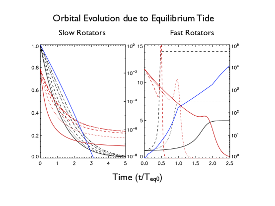
Figure 1.— Evolution of semi-major axis, a (black lines), and obliquity $\Theta$ (red lines) as a function of time for the equilibrium tide. Left axis represents semi-major axis and obliquity, right axis represents equilibrium timescale. Left hand panel show slow rotators (S/L$<$1), while the right hand panel shows fast rotators (S/L$>$1). $\Theta$ was initially set to 45^o in these integrations. Different linetypes represent different values of S/L.

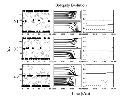
Figure 2.— Obliquity evolution of a population of objects with initially random obliquity and with $\tau_{10}/\tau_{eq}=0.001$. Left panels show the original random distribution of obliquities for the 50 objects (open circles), while filled circles show the distribution of obliquity after 30$\tau_{eq}$. Middle column shows the time evolution of the obliquity, while the right panel shows the fraction of objects as a function of time with prograde orbits (solid line), retrograde orbits (dotted line) and 90^o orbits (dashed line). In all scenarios the objects evolve to prograde, retrograde or 90^o orbits. Note that since we are keeping a fixed, S/L does not evolve.

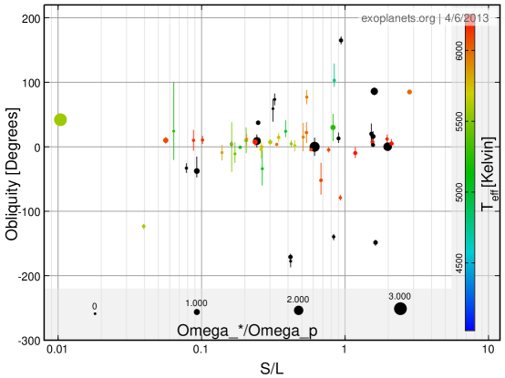
Figure 3.— Distribution of projected obliquity as a function of temperature, S/L and $\Omega_{\ast}/\Omega_{p}$. Cool stars are represented in color, while hot stars are represented in black.

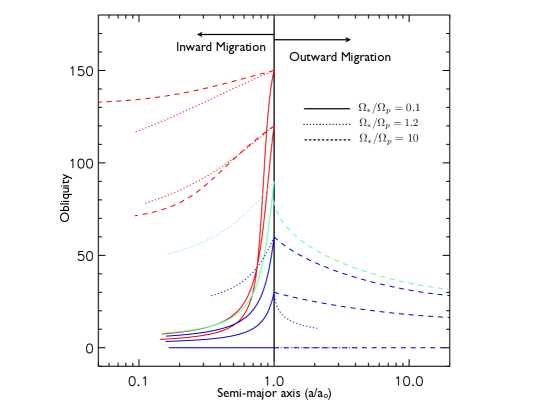
Figure 4.— Evolution of obliquity and semi-major axis for various ${\it initial}$ values of $\Omega_{\ast}/\Omega_{p}$, after 2$T_{eq0}$. Red, blue and green lines represent initially retrograde, prograde and 90^o orbits, respectively

References

- Albrecht et al. (2013) Albrecht, S., Winn, J. N., Marcy, G. W., Howard, A. W., Isaacson, H., & Johnson, J. A. 2013, eprint arXiv, 1302, 4443, ApJ, submitted
- Albrecht et al. (2012) Albrecht, S., et al. 2012, ApJ, 757, 18
- Alexander (1973) Alexander, M. E. 1973, Ap&SS, 23, 459
- Barker & Ogilvie (2009) Barker, A. J., & Ogilvie, G. I. 2009, MNRAS, 395, 2268
- Barker & Ogilvie (2010) Barker, A. J. & Ogilvie, G. I. 2010, MNRAS, 404, 1849
- Chatterjee et al. (2008) Chatterjee, S., Ford, E. B., Matsumura, S., & Rasio, F. A. 2008, ApJ, 686, 580
- Eggleton et al. (1998) Eggleton, P. P., Kiseleva, L. G., & Hut, P. 1998, ApJ, 499, 853
- Fabrycky & Tremaine (2007) Fabrycky, D., & Tremaine, S. 2007, ApJ, 669, 1298
- Goldreich & Nicholson (1989) Goldreich, P., & Nicholson, P. D. 1989, ApJ, 342, 1075
- Goodman & Lackner (2009) Goodman, J., & Lackner, C. 2009, ApJ, 696, 2054
- Greenspan (1968) Greenspan, H. 1968, The Theory of Rotating Fluids (Cambridge University Press)
- Hut (1980) Hut, P. 1980, A&A, 92, 167
- Ivanov & Papaloizou (2004) Ivanov, P. B., & Papaloizou, J. C. B. 2004, MNRAS, 347, 437
- Ivanov & Papaloizou (2007) —. 2007, MNRAS, 376, 682
- Lai (2012) Lai, D. 2012, MNRAS, 423, 486
- Lin et al. (1996) Lin, D. N. C., Bodenheimer, P., & Richardson, D. C. 1996, Nature, 380, 606
- Nagasawa & Ida (2011) Nagasawa, M., & Ida, S. 2011, ApJ, 742, 72
- Naoz et al. (2011) Naoz, S., Farr, W. M., Lithwick, Y., Rasio, F. A., & Teyssandier, J. 2011, Nature, 473, 187
- Ogilvie & Lesur (2012) Ogilvie, G. I., & Lesur, G. 2012, MNRAS, 422, 1975
- Ogilvie & Lin (2004) Ogilvie, G. I., & Lin, D. N. C. 2004, ApJ, 610, 477
- Ogilvie & Lin (2007) —. 2007, ApJ, 661, 1180
- Press & Teukolsky (1977) Press, W. H., & Teukolsky, S. A. 1977, ApJ, 213, 183
- Rasio & Ford (1996) Rasio, F. A., & Ford, E. B. 1996, Science, 274, 954
- Terquem et al. (1998) Terquem, C., Papaloizou, J. C. B., Nelson, R. P., & Lin, D. N. C. 1998, ApJ, 502, 788
- Winn et al. (2010) Winn, J. N., et al. 2010, ApJL, 723, L223
- Wu & Lithwick (2011) Wu, Y., & Lithwick, Y. 2011, ApJ, 735, 109
- Wu & Murray (2003) Wu, Y., & Murray, N. 2003, ApJ, 589, 605
- Zahn (1977) Zahn, J.-P. 1977, A&A, 57, 383