Multiperiodicity, modulations and flip-flops in variable star light curves

Abstract

Aims. According to earlier Doppler images of the magnetically active primary giant component of the RS CVn binary II Peg, the surface of the star was dominated by one single active longitude that was clearly drifting in the rotational frame of the binary system during 1994-2002; later imaging for 2004-2010, however, showed decreased and chaotic spot activity, with no signs of the drift pattern. Here we set out to investigate from a more extensive photometric dataset whether such a drift is a persistent phenomenon, in which case it could be due to either an azimuthal dynamo wave or an indication of the binary system orbital synchronization still being incomplete.

Methods. We analyse the datasets using the Carrier Fit method (hereafter CF), especially suitable for analyzing time series in which a fast clocking frequency (such as the rotation of the star) is modulated with a slower process (such as the stellar activity cycle).

Results. We combine all collected photometric data into one single data set, and analyze it with the CF method. As a result, we confirm the earlier results of the spot activity having been dominated by one primary spotted region almost through the entire data set, and the existence of a persistent, nearly linear drift. Disruptions of the linear trend and complicated phase behavior are also seen, but the period analysis reveals a rather stable periodicity with $P_{\rm spot}=$6^d.71054$\pm$0^d.00005. After the linear trend is removed from the data, we identify several abrupt phase jumps, three of which are analyzed in more detail with the CF method. These phase jumps closely resemble what is called flip-flop event, but the new spot configurations do not, in most cases, persist for longer than a few months.

Conclusions. There is some evidence of the regular drift without phase jumps being related to the high state, while complex phase behavior and disrupted drift pattern to the low state of magnetic activity. These findings do not support the scenario of the objects’ rotational velocity still being de-synchronized from the orbital period of the binary system. Neither is any straightforward explanation provided by the azimuthal dynamo wave scenario, as dynamo models preferentially show solutions with stable drift periods.

1 Introduction

II Peg is one of the most extensively studied SB1 RS CVn systems; recently, surface temperature (e.g. Berdyugina et al., 1998a, 1999; Gu et al., 2003; Lindborg et al., 2011; Hackman et al., 2012) and magnetic field maps have been published (Kochukhov et al., 2013; Carroll et al., 2007, 2009). The star’s photometric light curves have also been intensively studied with time series analysis and spot modelling methods (see e.g. Henry et al., 1995; Rodonò et al., 2000; Hackman et al., 2011; Roettenbacher et al., 2011), all the light curve variations being commonly interpreted being due to starspots (see e.g. the recent review by Strassmeier, 2009). One peculiar feature apparent especially from the paper by Lindborg et al. (2011) is the tendency of the magnetic activity to cluster on one primary active longitude, the position of which is linearly drifting in the orbital frame of reference of the binary system. Clustering of the spot activity on one single longitude has also been reported in other short-period eclipsing RS CVn systems e.g. by Zeilik & Budding (1987). In some earlier studies of II Peg (e.g. Berdyugina et al., 1999) indications of flip flops, i.e. the activity abruptly jumping from one longitude to another, separated roughly by 180 degrees, were reported, but the results of Lindborg et al. (2011); Hackman et al. (2012) did not give support to this interpretation.

Comparing with theoretical dynamo models (see e.g. Krause & Rädler, 1980; Rädler, 1975; Moss et al., 1995; Küker & Rüdiger, 1999; Tuominen et al., 2002), the drift was preliminarily associated with an azimuthal dynamo wave of the non-axisymmetric dynamo solution, resulting from dynamo action due to rotationally influenced turbulent convection without non-uniform rotation (so called $\alpha^{2}$ dynamo mechanism). Typically, the dynamo models predict dynamo waves either rotating faster or slower with a constant angular frequency over time. In addition to the dynamo wave changing its position in the phase-time plot, the solutions may exhibit oscillatory behavior concerning the energy level of the mean magnetic field, reminiscent of a stellar cycle. In a recent study of Mantere et al. (2013) the modelling showed that the drift cycle length (i.e. the time required for the non-axisymmetric magnetic structure to make a full rotation in the rotational frame of reference) and the oscillation period of the magnetic energy were always connected to each other. It has to be noted that in this particular study, only a very small fraction of the parameter space was mapped, within which solutions for which the drift cycle length and oscillation of the magnetic energy levels coincided were found to be preferred. Flip-flop type switches have been found in dynamo models, where relatively small amounts of differential rotation have been allowed for (so called $\alpha^{2}\Omega$ modes, see e.g. Elstner & Korhonen, 2005; Korhonen & Elstner, 2011). In these models, flip-flops result from the competition of oscillatory axisymmetric mode and the stable non-axisymmetric mode of comparable strengths.

II Peg belongs to a binary system, the rotational speed of which can be deduced from radial velocity measurements (e.g. Berdyugina et al., 1998b). It is well known that the tidal effects due to the presence of the companion star will circularize the orbit of the binary system and force the rotation of the star to be synchronised to the orbital period of the binary in a time frame of a billion years after settling to the main sequence (see e.g. Zahn & Bouchet, 1989). In the case of the rotation of the star not yet being fully synchronised, i.e. the rotational speed still being larger than implied by the orbital period of the binary, one would expect a systematic drift of the lightcurve minima when wrapped with the binary period; this constitutes the second possible explanation to the drift of the spots on the star’s surface. If this was the case, a persistent drift of the activity tracers, making the stellar surface and rotation visible to the observer, over the whole extent of the time series should be seen - the amplitude of the spottedness or the magnetic field strength could still vary, but the drift should still be visible if this amplitude variation was removed. In contrast to the dynamo wave scenario presented above, no obvious connection between the drift versus the modulation should be visible.

Intriguingly, the drift was no longer visible in the Doppler (hereafter DI) and Zeeman Doppler images (hereafter ZDI) of Hackman et al. (2012) and Kochukhov et al. (2013), who also reported on the clear diminishing trend in the spottedness and magnetic field strength of the object. This was interpreted as the star’s activity declining towards its magnetic minimum, due to which the spot distribution on the stellar surface was postulated to be more stochastic than during the high activity state, veiling the possible drift due to the mechanism producing it underneath. We note that the results of Carroll et al. (2007, 2009), computed from the same data with a different ZDI inversion method (Carroll et al., 2008), also indicate a reduction in the magnetic field strength between the observing seasons 2004 and 2007. They, however, report that a dominant and largely unipolar field seen in 2004 changed into two distinct, large-scale, bipolar structures in 2007, not completely consistent with the proposed picture of the star declining towards its magnetic minimum with less pronounced, stochastic spot activity.

Based on these analyses, however, it is not possible to fully rule out the scenario of the drift having really disappeared. A time-dependent drift period would not match either of the two proposed scenarios, and would be an important finding as such.

Whichever the cause or persistence of the drift, this type of a problem is especially suited to be analyzed with the recently developed Carrier Fit (CF) analysis method (Pelt et al., 2011), which is based on the idea of continuous fitting of the time series (e.g. a light curve of a star) clocked by a certain shorter carrier period (or larger frequency) while being modulated by a longer period (or smaller frequency). This method has already successfully been applied to analyze the phase changes seen in the light curve of FK Com (Hackman et al., 2013). In the case of II Peg, the orbital period of the binary system serves as the first guess of the carrier period, while the apparent modulation of the amplitude of the spots and/or magnetic field present the modulation period. If either of the proposed scenarios (azimuthal dynamo wave, orbital de-synchronization) would be true, we should be able to find a persistent drift period. The two mechanisms could be differentiated from each other by examining the correlation of the modulating period to the carrier; while the dynamo scenario might show up as these two being connected, the other scenario would imply no connection. Another method with which these hypothesis could be tested would be to use a ’local’ period search method with a sliding window, such as the CPS method of Lehtinen et al. (2011), which would allow the comparison of the mean active longitude rotation period to the short-term photometric period.

In this paper, we aim to investigate the drift phenomenon in detail, combining all the available photometry of the star into our analysis. The primary goal of this paper is to study whether a systematic drift period persisting over time exists with the CF method. In Sect. 2 we introduce the data used, in Sect. 3 present a short summary of the CF method, in Sect. 4 present our results, in Sect. 5 compare the photometric results to earlier Doppler images, and in Sect. 6 summarize and discuss the possible implications of the results obtained.

2 Photometric datasets

We use four different data sets for our CF analysis. The first data set (hereafter DATA1), published and analyzed by Rodonò et al. (2000), covers the years 1973-1998. The second data set (hereafter DATA2) was published by Messina (2008) covering the years 1992-2004, therefore partly overlapping with DATA1. The third data set (hereafter DATA3) consists of unpublished observations with the Wolfgang-Amadeus, the university of Potsdam/Vienna twin automatic photoelectric telescope (APT), covering the years 1996-2009, again partially overlapping with the previous datasets. The fourth dataset (hereafter DATA4) was obtained with the Tennessee State University T3 0.4-m Automated Photometric Telescope at Fairborn Observatory in Arizona, covering the time span of 1987-2010 (see also Roettenbacher et al., 2011, for another analysis of the same dataset). These datasets are combined, to collect as extensive a dataset as possible, with the densest possible coverage of observations. The combination was done by shifting the magnitudes and rescaling the amplitudes to get the best match in overlapping areas. The quality of the match was measured by computing mean-squared differences between magnitudes in data point pairs where the time distance was less than 0.2 days. The optimal scaling shift and magnitude corrections were obtained by a least-squares minimization. The first six years of DATA1 (1973-1979) have gaps in time too wide for the CF analysis so these data were removed from the combined data set (see Fig. 1). We also divided the combined dataset into shorter segments, either to look for phase jumps or flip-flop type events, following the ideas presented in Hackman et al. (2013), or to be able to identify the best period describing the drift of the primary light curve minimum in the orbital frame of reference.

Figure 1: All the photometric data normalized and combined.

3 The Carrier Fit method

Astronomical data is complicated for a straightforward Fourier analysis, because the observed light curves and spectra usually have long time gaps between observations. This makes the analysis difficult and creates false peaks due to the regularities in the gap structure of the input data (see e.g. the review by Schwarzenberg-Czerny, 2003, and references therein). Pelt et al. (2011) developed a novel method for stellar light curve analysis, based on a simple idea of decomposing the light curve into two separate components: a rapidly changing carrier tracing the regular part of the signal, and its slowly changing modulation. The carrier frequency can be obtained from observations (e.g. the period can be obtained from rotational velocity) or estimated from the data as a mean frequency. The smooth modulation curves are described by trigonometric polynomials or splines. For a complete description of the method we refer to Pelt et al. (2011) and as another practical application for stellar light curves to Hackman et al. (2013, analysis of FK Com); here we merely highlight the most important input quantities and properties of the method.

The proposed composition of the light curve is described with the following formula:

$$f(t)=a_{0}(t)+\Sigma^{K}_{k=1}(a_{k}(t)\cos(2\pi tk\nu_{0})+b_{k}(t)\sin(2\pi tk\nu_{0})),$$ (1)

where $\nu_{0}$ is the carrier frequency, $a_{0}(t)$ is the time-dependent mean level of the signal, $K$ is the total number of harmonics included in the model, describing the overtones of the basic carrier frequency, while $a_{k}(t)$ and $b_{k}(t)$ are the low-frequency signal components. In the case of II Peg, the first guess of the carrier frequency $\nu_{0}=P_{0}^{-1}$ comes from the consideration of the system being a binary system, most likely with synchronized orbits of the components. Therefore, we adopt the orbital period of the binary system, $P_{0}$=6^d.724333, estimated by Berdyugina et al. (1998b) as the first carrier. The next task of the analysis is to choose a suitable model for the modulators. In Pelt et al. (2011) we proposed two different types of models based on either trigonometric or spline approximation. The II Peg light curve contains fairly small amount of complicated features, making the usage of the trigonometric model adequate.

We build the trigonometric modulator model in the following way: Let the time interval $[t_{\min},t_{\max}]$ be the full span of our input data, based on which we define a data period $D=C\times(t_{\max}-t_{\min})$, where $C$ is a so called coverage factor, the value of which must be larger than unity. Next we construct a truncated trigonometric series using the corresponding data frequency, $\nu_{D}=1/D$, i.e.:

$$a(t)=c_{0}^{a}+\sum\limits_{l=1}^{L}{\big{(}c_{l}^{a}\cos(2\pi tl\nu_{D})+s_{l}^{a}\sin(2\pi tl\nu_{D})\big{)},}$$ (2)

and

$$b(t)=c_{0}^{b}+\sum\limits_{l=1}^{L}{\big{(}c_{l}^{b}\cos(2\pi tl\nu_{D})+s_{l}^{b}\sin(2\pi tl\nu_{D})\big{)},}$$ (3)

where $L$ is the total number of harmonics used in the modulator model. The process described by the modulators and data period $D$ must be slow, i.e. $D$ must be significantly longer than the carrier period $P_{0}$. The data of each set span over several thousands of days, due to which we conclude that 10000 days is an appropriate value for the data period; the corresponding coverage factors are roughly $C$=1.2, well in the range considered to be satisfactory $C=1.1\ldots 1.5$ (see Pelt et al., 2011).

Next, proper estimates for the expansion coefficients are computed for every term in the series for the fixed carrier frequency $\nu_{0}$ and $D$; this is a standard linear estimation procedure and can be implemented using any standard statistical package (see Pelt et al., 2011, for detailed description). If all coefficients ($a_{k},b_{k}$) consist of the same number of harmonics $L$ and we approximate separate cycles by a $K$-harmonic model, then the overall count of linear parameters to be fitted is $N=(2\times L+1)\times(2\times K+1)$. The optimal number of harmonics, $K$, depends on the complexity of the phase curves. The choice of the optimal number of modulator harmonics, $L$, is constrained by the longest gaps in the time series. As the light curve of II Peg appears not to be very complicated, as discussed at length in Sect. 4, we find $K=3$ and $L=12$ adequate for the analysis of the combined data set (Stage 1). For the short segments the number of data points tends to be small and therefore we choose $K=2$ (instead of $K=3$) and $L=3$ to reduce the number of model parameters (Stage 3).

Finally, we have found it convenient to visualize our results in the following way. We begin with calculating a continuous curve estimate, $\hat{y}(t)$, from the randomly spaced data set containing gaps, using a least-squares fitting scheme based on the carrier frequency. As a result, we can also model the gaps between the data, which allows us to get a smooth picture of the long-term behaviour. The continuous curve is then divided into strips, the length of each being the carrier period. Each data strip is then normalized with its extrema, so that after the normalization the data spans the range of $[-1,1]$. We note that without this normalization procedure, epochs of weaker spot activity, showing up as less variation in the light curve, would be drowned in the signal from strong spot activity epochs. Finally, after normalization, we collect the strips along the time axis. To facilitate the interpretation of the plots, we do not restrict them to the interval of $[0,1]$ over phase, but extend our phase axis to somewhat larger and smaller values. At the bottom of the plots we show the time distribution of the actual observations in the form of a “bar code”. The black stripes are used to denote periods during which at least one observation is available, while the bright stripes represent gaps. This method of visualisation allows us to verify that the model correctly fits into the data rather than into the gaps.

4 The CF analysis procedure and results

During the first stage of our investigation, we perform the CF analysis for the combined dataset (Fig. 1) as a whole. As previous photometric and spectroscopic investigations have already suggested, we find one single photometric minimum, i.e. one large spotted region, dominating the light curve almost for the entire span of the data. This region often exhibits a linear downward trend in the phase diagram that is wrapped with the orbital period, indicating that it is rotating somewhat faster than the orbital period of the binary system. During some epochs, this trend is disrupted for some years, but it appears again. Therefore, we set out to determine this period, which can be thought to describe either the rotation of the spotted region on the surface of the object or the signature of an underlying magnetic structure feeding the surface; this constitutes the second stage of our analysis. In the third stage, we locate all the epochs during which significant deviations from the drift trend can be seen. We zoom into these epochs, and perform a more detailed CF analysis on them, to be able to conclude on the nature of the more complex phase behavior occasionally seen on the object.

4.1 Stage 1: analysis of the combined dataset

We begin by analyzing the whole combined dataset [DATA1,DATA2,DATA3,DATA4], i.e. all the data points in Fig. 1 excluding only the very early points with too large gaps during 1973-1978. The CF analysis results with $P_{0}$=6^d.724333, $C$=1.15, number of carrier harmonics $K$=3 and modulation harmonics $L$=12 is depicted in Fig. 2. The linear downward trend in the orbital frame is well visible especially during the years 1995–2005 (subinterval of DATA3 and DATA4), and evidently present also during the years 1979-1988 (subinterval of DATA1 and DATA2). In the early part of the data, however, the phase of the principal light curve minimum is alternating around the phase of the mean trend, with seemingly regular timing. Moreover, the phase jumps seem to occur rather abruptly.

During the time interval of 1988-1995, the linear trend is visibly disrupted, manifested by the phase of the principal minimum staying constant in the orbital frame for these years. In 1995, the linear trend, however, resumes with a roughly equivalent period to the earlier years. After 2005, a similar disruption is seen again, followed by very complex behavior in the end of the data set.

In summary, four main features can be isolated from the first stage of our analysis:

• The data is dominated by one single light curve minimum, i.e. one spotted region, almost the entire span of the data.

• There is a linear downward trend with a period faster than 6^d.724333, visible during 1979-1988 and 1995-2005.

• Disruptions of the linear trend occur during 1988-1995 and 2005-2010.

• Some abrupt phase jumps are seen, not directly correlated with either the presence/absence of the linear trend.

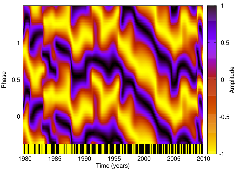
Figure 2: Continuous fit of to the combined dataset from CF analysis with carrier $P_{0}$.

4.2 Stage 2: finding the drift period

The next task is to estimate the period that best describes the linear trend seen in the dataset, $P_{\rm spot}$. As already evident from the first stage of the analysis, the trend is not visible at all times of the data, meaning that the period is not a completely stable one.

Suitable methods to estimate light curves with significant deviations from harmonic behavior are based on phase dispersion minimization. The Stellingwerf method (Stellingwerf, 1978) is among the best known of such methods, and is used in the following as our base method for period search. However, the method should be refined to be capable of dealing with a periodicity that is not completely time independent and stable. For this purpose a more general formulation of the phase dispersion is needed. In this work we introduce a variant of the statistic proposed earlier by Pelt (1983) that is referred to as Method 2 in the remaining of the paper. Specifically, for each trial period $P$ we compute the dispersion of phases wrapped with this particular period as

$$D(P)=\frac{{\sum\limits_{i=1}^{N-1}{\sum\limits_{j=i+1}^{N}{g(t_{i}}},t_{j},P,\Delta t)[f(t_{i})-f(t_{j})]^{2}}}{{\sum\limits_{i=1}^{N-1}{\sum\limits_{j=i+1}^{N}{g(t_{i}}},t_{j},P,\Delta t)}},$$ (4)

where $g(t_{i},t_{j},P,\Delta t)$ is significantly greater than zero only when

$$t_{j}-t_{j} \approx kP,k=\pm 1,\pm 2,\ldots{\rm\ \ \ and}$$ (5)

$$\left|{t_{j}-t_{j}}\right| \leq \Delta t.$$ (6)

The first condition selects only the data point (magnitude) pairs $[f(t_{i})$,$f(t_{j})]$ the phases of which are approximately the same and the second condition restricts the time interval of the selected data points to a certain pre-selected time range $\Delta t$. By computing $D(P)$ for a sequence of trial periods we get the phase dispersion spectra. The minima in these spectra indicate probable periodicities; due to the normalization the expected $D(P)$ value for randomly scattered phase diagrams is 2. For the particular case when the time difference limit is longer than the full data span the obtained spectra practically coincide with traditional Stellingwerf spectra. By making the time limit $\Delta t$ shorter we can analyse phase scatter for the case when different cycles match each other only locally; for the present analysis, we find $\Delta t$ of 300 days optimal. In this case the final minimum in the $D(P)$ spectrum indicates a certain estimate of the mean cycle length (mean period). In this way we can analyse data sets that are not coherent during the full data span but only locally.

It is reasonable to compute Stellingwerf and $D(P)=D(1/\nu)$ spectra with a fixed step along the frequency $\nu$. The optimal step size,

$$\Delta\nu={0.05\over t_{max}-t_{min}},$$ (7)

limits the phase change from one trial to the next by an upper limit of $0.05$ for all pairs along the full time span $[t_{min},t_{max}]$. The distance between neighbouring periods depends on the period argument $P$

$$\Delta P=P^{2}\Delta\nu.$$ (8)

This value can roughly be used to characterize the precision of the obtained period estimates.

The exact error estimates and significance levels for the estimated mean periods can be computed by using either standard regression techniques, Monte Carlo type methods, the Fischer randomization technique or bootstrap. However, we note that these are only formal error estimates. The real scatter of the mean period heavily depends on the physics involved and to estimate it we need significantly longer data sets than the ones available for this study. In our particular case we used the standard regression analysis method to estimate the errors of the final period. We iteratively refined the obtained period and used a correlation matrix to compute the dispersion of the refined period.

Method	Data	Period $P$[d]	$\Delta P$
Stellingwerf	All	6.7108	0.0002
Method 2	All	6.7106	0.0002
Stellingwerf	Subset	6.7109	0.0004
Method 2	Subset	6.7109	0.0004

Table 1: Periods derived for combined and subsets of the data with two different methods.

The Stellingwerf periodogram for the full dataset, plotted with the thinnest gray line in Fig. 3, shows the shallowest minimum split into several peaks. The form of the spectrum does not change when the correlation length is decreased using Method 2, but the minimum gets deeper (2nd thinnest gray line). This is an indication supporting the hypothesis that the period is not completely stable. For the subset with the clearest linear trend seen in the phase diagram, the spectrum is characterized with only one clear peak in the periodogram with both methods (two thickest lines). Decreasing the correlation length again using Method 2 makes the minimum deeper (the thickest line).

Most importantly, the best period is practically the same for both datasets analysed with either method. This is an indication of the trend dominating in the data, despite of the disruptions and phase jumps additionally seen in it occasionally. Therefore, we can pin down the rotation period of the spotted region to be $P_{\rm spots}=$6^d.71086$\pm$0^d.00007, the value of the period obtained after the least-squares refinement of the initial estimate. The phase diagram, wrapped with the new period, is shown in Fig. 4. This figure reveals quite a different picture from the phase diagram wrapped with the orbital period - the trend having been removed, the primary minimum mainly stays on one straight line at phase 0.5, although smooth variability up and down can be seen. The phase changes around the mean drift period during the early part of the data (1979-1990) now look fairly similar to the fluctuations seen in the later part with a clear trend (1995-2005). Abrupt phase jumps are more easy to identify; three major events can be seen during 1984-1985, 1990-1991, and 2009-2010. Next, we concentrate on investigating the phase jumps in more detail.

Figure 3: Periodograms from two different methods with two different datasets.

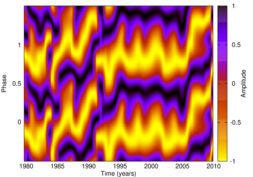
Figure 4: Phase diagram with the new carrier, $P_{\rm spot}=$6^d.71086.

4.3 Stage 3: analysis of short segments

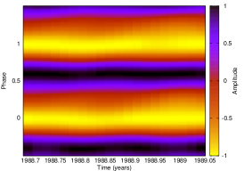
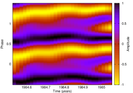
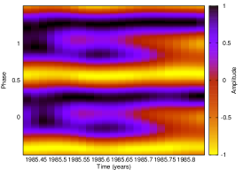
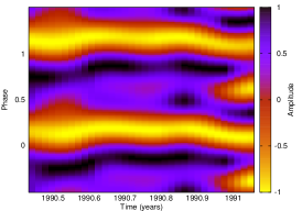
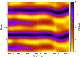
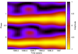
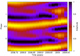
Figure 5: Panel in the top row shows SEG12 as an example of a segment with stable phase behavior. Lower rows: Zoom-in to segments in which phase changes were detected. From left to right, top to bottom, SEG07, SEG08, SEG14, SEG15, SEG20 and SEG39.

Next, we divide the data into shorter segments, and perform a ’local’ CF analysis (see also Hackman et al., 2013, for similar analysis). The division of the data into segments was done according to the following rules: We started to group the data from the first point of the combined data set. The next point of the data was included in the same segment, until a gap longer than 60 days was encountered; this was found to be the absolute maximum for gap length without spoiling the CF analysis. Then the current segment was considered to be completed, and a new one started. This way, altogether 42 segments of varying length and number of data points were formed, but 19 of them contained too few points to allow for a meaningful CF analysis. The remaining segments were analyzed with the CF method using $K=2$ and $L=3$ and utilizing the refined carrier period $P_{\rm spot}$. Most of the segments show very little variation in phase over time; the segments can be well described with a horizontal stripe, i.e. the principal minimum stays at the same phase. As an example of practically no phase change we show SEG12 in Fig. 5, first panel; segments resembling this one are indicated with ’-’ (no change) in Table 4.3.

Only four of all the 23 segments containing enough points allowing for a local CF analysis (SEG07, SEG08, SEG14, SEG39) show clear, abrupt phase changes. In addition, two of the segments, namely SEG15 and 20, show disrupted phase behavior, which cannot well be described as phase jumps (indicated with ’?’ in Table 4.3). The two first segments showing interesting behavior (SEG07 and SEG08) are connected to the epoch of phase disturbance seen during 1984-1985. Comparing Figs. 4 and 5 (second and third upper panel) it seems evident that during 1979-1984, the activity has been ’wobbling’ around the ’mean’ phase of 0.25, the location of which roughly agrees with the linear trend, i.e. stays horizontal in Fig. 4. During 1984-1985, a series of more abrupt phase jumps are observed to occur, with two short-lived transitions between phases 0.2 and 0.6. After a third abrupt transition in the middle of 1985, the major part of the activity has remained at the new phase of 0.6 (although hints of a secondary minimum being active at 0.25 can be seen in the global phase diagram) until 1990, the ’mean’ phase of activity again being consistent with the overall linear trend. Another phase jump can be seen in SEG14, in the end of the year 1990, when the main activity seems to have quickly reverted back to the phase of roughly 0.2, but this spot configuration appears unstable, reverting back to phase 0.6 via a continuous phase drift during 1992-1995. The last abrupt phase jump is seen in SEG39, close to the end of the dataset. Again, a change of roughly 0.5 in phase can be identified.

To conclude, the characteristics of the phase jumps rather closely resemble what is called the flip-flop (Jetsu et al., 1993), i.e. the activity shifts roughly 0.5 in phase within a time scale of a few months. The last jump (in SEG39) occurred very near the endpoint of the time series, due to which it is difficult to conclude about the persistence of the spot configuration after the event; only one of the other new spot configurations after a flip-flop type event, seen during 1985, seems to have persisted over a longer period of time (several years), while the others have either flipped or drifted back to the original configurations soon afterwards.

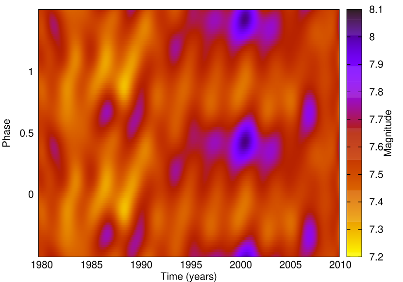
Figure 6: CF phase diagram with no normalization.

There is a ten-year long time interval when the abrupt phase jump activity clearly ceases to occur (1995-2005), during which only the linear drift, and some ’wobbling’ around the mean phase, is seen. From spectroscopy (covering the time 1994-2010 Lindborg et al., 2011; Hackman et al., 2012) and spectropolarimetry (Kochukhov et al., 2013, covering the time 2004-2010) there is some evidence of the star’s magnetic field strength getting weaker and the spots more randomly distributed over phase during the latest epoch of disturbed phase activity (2004-2010). The chosen CF visualization scheme of normalizing each stripe with its own extrema acts to hide possible amplitude variations in our photometric analysis. Therefore, we re-compute the phase diagram wrapped with $P_{\rm spot}$ without using this normalization, the result being shown in Fig. 6. From this plot it is evident that the photometric minima are indeed deeper during the period of the most pronounced linear trend, whereas irregular phase behavior and flip-flop type events are related to the epoch of weaker photometric minima. On the other hand, it is noteworthy that the mean photometric magnitude of the star stays approximately constant after the year 1990 (see Fig. 1), while only the strength of the variations around the mean are larger during the epoch with the most pronounced linear trend. The constant mean level of the photometric magnitude is suggestive of the overall magnetic activity level of the star having remained unchanged, while the activity is distributed less axisymmetrically during the epoch of large magnitude variations.

Segment	$N$	$\Delta t$	Events
SEG01	27	102.9	NA
SEG02	48	97.0	NA
SEG03	60	130.7	NA
SEG04	17	76.0	NA
SEG05	16	40.0	NA
SEG06	43	88.8	NA
SEG07	78	201.9	+
SEG08	98	167.8	+
SEG09	62	153.5	NA
SEG10	39	87.3	NA
SEG11	3	5.0	NA
SEG12	130	145.2	-
SEG13	166	248.6	-
SEG14	85	237.6	+
SEG15	108	257.6	?
SEG16	149	219.6	-
SEG17	180	248.6	-
SEG18	151	257.6	-
SEG19	329	255.6	-
SEG20	359	259.6	?
SEG21	567	265.6	-
SEG22	80	32.9	NA
SEG23	308	147.8	-
SEG24	318	267.3	-
SEG25	219	246.6	-
SEG26	24	23.0	NA
SEG27	201	158.1	-
SEG28	322	254.6	-
SEG29	49	46.9	NA
SEG30	253	148.8	-
SEG31	58	41.9	NA
SEG32	229	149.8	-
SEG33	285	260.6	-
SEG34	37	40.0	NA
SEG35	196	138.8	-
SEG36	41	31.0	NA
SEG37	172	131.9	-
SEG38	28	29.0	NA
SEG39	163	136.8	+
SEG40	9	17.0	NA
SEG41	48	130.6	NA
SEG42	6	15.0	NA

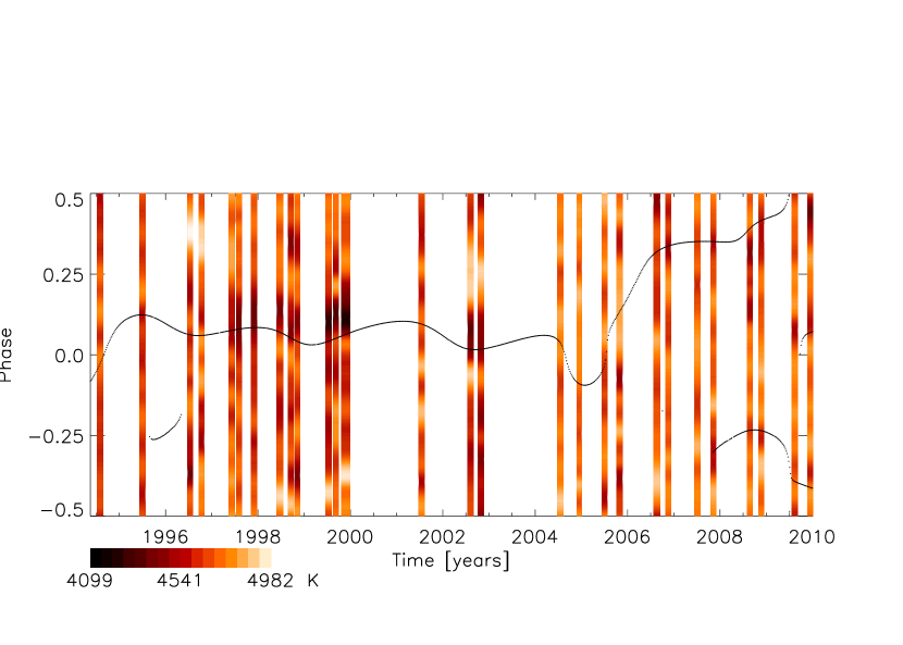
Figure 7: Temperature distribution over phase (y-axis) plotted as function of time (x-axis) calculated as averages over all latitudes from the surface temperature maps obtained with Doppler imaging. The black crosses indicate the phases of the photometric minima obtained from the CF analysis. The phases are wrapped with the best period describing the linear trend, $P_{\rm spot}$ using the first timepoint of DI observations as the epoch.

5 Comparison with recent temperature maps

In this section we compare the temperature minima obtained from Doppler imaging (DI) by Hackman et al. (2011) to the photometric results; altogether 28 surface temperature maps of the object were derived in this paper for the years 1994-2010. For comparison purposes, in Fig. 7 we plot the latitudinally averaged temperature profiles of the DI maps as function of time, but in contrast to earlier studies (see e.g. Hackman et al., 2011), we wrap the phases with the $P_{\rm spot}$ that was found to describe the linear drift of the photometric minima. As evident from this figure, one large primary spot, seen as extensive dark patches in the color contour, was seen on the object during 1997-2002, the phases of which evolve along rather a horizontal line when wrapped with $P_{\rm spot}$. During the epochs 1994-1997 and 2004-2010 weaker spot activity, the spots being randomly distributed over the stellar longitude, is seen. The photometric minima from our analysis, plotted on top of the DI results with black crosses, closely coincide with the DI minima for the years with pronounced spot activity, while the differences are greater for the other epochs. Comparing to the earlier investigation of Hackman et al. (2011) using a different time series analysis method for the photometric data, we find the results to be in a fair agreement. Therefore we conclude that the linear drift pattern is a robust feature seen both in the DI maps and photometric data analyzed with different types of methods, persisting at least over a ten year epoch during 1995-2005. The DI maps, on the other hand, do not show any clear evidence of the rather continuous phase drift seen during 2005-2009 or the abrupt phase jump detected from photometry in the end of the dataset (during 2010 in SEG39).

6 Summary and discussion

We have collected a 21-year long photometric data set of the magnetically active primary giant component of the RS CVn binary II Peg, and analyzed this data set with the CF method, both globally and locally. As a result, we confirm the earlier results of the spot activity having been dominated by one primary spotted region almost through the entire data set, and the existence of a rather persistent linear drift. Disruptions of the linear trend and complicated phase behavior are also seen, but the period analysis reveals a periodicity with $P_{\rm spot}=$6^d.71086$\pm$0^d.00007. After the linear trend is removed from the data, we identify several abrupt phase jumps, three of which are analyzed with the CF method using shorter data segments. These phase jumps closely resemble what is called the flip-flop event, i.e. the spot activity changes by roughly 0.5 in phase within months, but only one of the phase jumps leads to a stable spot configuration persisting over several years. In other cases, flips back or more continuous drifts towards the original spot configurations are seen.

The comparison to Doppler imaging temperature maps confirms the existence of the linear drift pattern with regular phase behavior for the epoch 1995-2005, during which the level of spot activity of the star has been high. During the epochs when photometric analysis shows disrupted phase behavior and phase jumps, the Doppler images show weak spots randomly distributed over the longitudes. Therefore, there is some evidence of the regular drift without phase jumps being related to the high state, while complex phase behavior and disrupted drift patterns to the low state of spot activity. The Zeeman Doppler imaging results of Kochukhov et al. (2013) indicate the magnetic field strength of the object getting weaker on average since 2004. The mean photometric brightness of the object, however, has remained more or less constant since 1990, suggesting that the overall magnetic activity level has not changed considerably, although the variations around the mean have been higher during the epoch of the pronounced linear trend.

Although the periodicity describing the drift of the primary spot in the orbital frame of reference of the binary system is stable in a statistical sense, the trend is clearly disrupted during the epochs of complex phase behavior; this casts serious doubt of the primary light curve minimum reflecting the actual, more rapid, rotation of the primary component of the binary system, that would indicate that the rotation rates of the stars would still remain de-synchronized by the mutual tidal forces. Also practically all the dynamo models produced up to date (see e.g. Krause & Rädler, 1980; Küker & Rüdiger, 1999; Moss et al., 1995; Tuominen et al., 2002; Mantere et al., 2013) show stable drift periods, making it equally hard to explain the results obtained in this work with the azimuthal dynamo wave scenario. We note, however, that the recent models of Mantere et al. (2013) indicate that the oscillations in the magnetic activity level should be connected to the cycle length of the drift of the non-axisymmetric structures. Using the drift period $P_{\rm spot}$ obtained in this work, an oscillation in the magnetic energy level with a period of

$$P_{\rm mag}=\frac{P_{0}-P_{\rm spot}}{P_{0}P_{\rm spot}}\approx 9.2\ {\rm years}$$ (9)

would be expected. To test this scenario further, however, is out of the scope of this study.