Gravitational redshifts from large-scale structure

Abstract

The recent measurement of the gravitational redshifts of galaxies in galaxy clusters by Wojtak et al. has opened a new observational window on dark matter and modified gravity. By stacking clusters this determination effectively used the line of sight distortion of the cross-correlation function of massive galaxies and lower mass galaxies to estimate the gravitational redshift profile of clusters out to $4\;h^{-1}{\rm Mpc}$ Here we use a halo model of clustering to predict the distortion due to gravitational redshifts of the cross-correlation function on scales from $1\sim 100\;h^{-1}{\rm Mpc}$. We compare our predictions to simulations and use the simulations to make mock catalogues relevant to current and future galaxy redshift surveys. Without formulating an optimal estimator, we find that the full BOSS survey should be able to detect gravitational redshifts from large-scale structure at the $\sim 4\sigma$ level. Upcoming redshift surveys will greatly increase the number of galaxies useable in such studies and the BigBOSS and Euclid experiments should be capable of measurements with precision at the few percent level. As has been recently pointed out by McDonald, Kaiser and Zhao et al, other interesting effects including relativistic beaming and transverse Doppler shift can add additional asymmetric distortions to the correlation function. While these contributions are subdominant to the gravitational redshift on large scales, they represent additional opportunities to probe gravitational physics and indicate that many qualitatively new measurements should soon be possible using large redshift surveys.

1 Introduction

In the weak field limit, the gravitational redshift, $z_{g}$ of photons with wavelength $\lambda$ emitted in a gravitational potential $\phi$ and observed at infinity is given by $z_{g}=\frac{\Delta\lambda}{\lambda}\simeq\frac{\Delta\phi}{c^{2}}$. Measurement of $z_{g}$ is one of the fundamental tests of General Relativity (GR). First measured more that 50 years ago for the Earth’s gravity in a laboratory setting (Pound & Rebka 1959), subsequent determinations have been made in the solar system (Lopresto et al. 1991) and from spectral line shifts in red giant stars (e.g., Greenstein et al. 1971). In this paper we will examine how well the gravitational redshifts caused by the largest potential fluctuations in the Universe can be measured using galaxy redshift surveys.

Predictions for the gravitational redshifts of galaxies in clusters were computed using analytic models by Cappi (1995, see also Nottale 1990). Cappi found that in the most massive ($\lower 2.15277pt\hbox{$\;\buildrel>\over{\sim}\;$}10^{15}{h^{-1}M_{\odot}}$) clusters the central galaxy is expected to have a redshift of a few tens of ${\rm\;km\;s^{-1}}$ with respect to other cluster members. Kim & Croft (2004, hereafter KC04) showed that instead of using single extremely massive clusters, large galaxy surveys could be used to make a statistical measurement of the gravitational redshift profile. McDonald (2009, hereafter M09) examined the issue in Fourier space and pertubation theory, studying the effect of gravitational redshifts on the large-scale cross-power spectrum of different populations of galaxies.

The first observational determination of galaxy gravitational redshifts due to their large-scale environment was made by Wojtak et al. (2011, hereafter W11) using galaxy redshift data from the Sloan Digital Sky Survey (SDSS). W11 used 125000 galaxies in 7800 galaxy clusters to make statistical measurement of $z_{g}$ vs. brightest cluster galaxy distance out to a radius of $4\;h^{-1}{\rm Mpc}$ ($h=H_{0}/100{\rm\;km\;s^{-1}}\;{\rm Mpc}^{-1}$). Their $2.6\sigma$ measurement was compared to modelling of the mass distribution from galaxy velocity dispersions and used to put constraints on modified gravity models. Dominguez-Romero (2012) also used SDSS data to carry out such a test and also found good agreement with GR.

The redshift of a galaxy is a sum of 3 components, the Hubble redshift, the Doppler redshift from the line of sight peculiar velocity and the gravitational redshift:

$$cz=H(z)r+v_{\rm pec}+cz_{g},$$ (1)

where $H(z)$ is the Hubble parameter and $r$ the radial distance between the observer and galaxy in Mpc. The autocorrelation function of galaxies is often measured as a function of separation between pairs of galaxies along the line of sight ($r_{\parallel}$) and across it ($r_{\perp}$). The $v_{\rm pec}$ and $cz_{g}$ terms in Equation 1 distort the correlation function of galaxies in the $r_{\parallel}$ direction. For the autocorrelation this distortion is symmetric about $\Delta(r_{\parallel})=0$. However, more highly clustered galaxies (in practice also more massive) lie in deeper potential wells and so have a higher $cz_{g}$ on average than less clustered (and less massive) galaxies. This means that the cross-correlation function of two subsets of galaxies with different clustering strengths will be asymmetric about the $r_{\perp}$ axis. If the cross-correlation function is centered on the most massive galaxy the surrounding galaxies will have an relative blueshift. This blueshift can be measured as a function of galaxy pair separation and therefore provide a measure of the scale dependence of the large scale gravitational potential around galaxies.

The cross-correlation can be carried out between any subsets of galaxies. In KC04 and W11 the higher mass subset were brightest cluster galaxies (BCGs) and the lower mass subset were other cluster members and nearby field galaxies. M09 considered two general populations of galaxies with different bias parameters and showed that in Fourier space the gravitational redshift leads to an imaginary term in the cross-spectrum. The analysis of M09 was carried out in linear theory, but also included other terms in the distortion of clustering (related to the transformation from observable to proper coordinates, see Yoo et al. 2009,2011). Our current study will include non-linear scales and make use of N-body simulations to formulate and test the simplest measurement scheme. Our aim is to be able to unify the two regimes that were considered previously, virialized objects and large scale linear structure and formulate a model and analysis method applicable to all scales.

Because the predicted gravitational redshift of galaxies is typically much smaller than the other terms in Equation 1, there are several other effects which need to be considered when devising a scheme to measure $z_{g}$ from galaxy clustering. Most of these effects have been considered in the context of galaxy clusters and are most important in virialized regions. For example, Zhao et al. (2012) have shown that that because the galaxies around the cluster center are not at rest, special relativistic time dilation leads to an additional wavelength shift between those and the center (BCG in the case of a cluster). Zhao et al. term this the Transverse Doppler effect and point out that it will be opposite in sign to $z_{g}$. Kaiser (2013, hereafter K13) recently explored several more effects, including special relativistic beaming which will cause infalling galaxies behind a cluster to be brighter. This will boost the number above a magnitude limit behind a cluster compared to in front and give an asymmetry of similar order to the $z_{g}$ effect. K13 (see also KC04) also considered the cluster in the context of an infalling density field that joins the Hubble flow at large radii. This and the effects explored in M09 can in principle be modelled and marginalized over when looking the effect of gravitational redshifts, so that we leave a detailed study of their properties to future work. We give some comments on their likely relative magnitude and other potential effects in Section 5.2 but in the present paper we concentrate on predictions for $z_{g}$.

Our our plan for the paper is as follows. In Section 2 we use halo model-inspired fits to the galaxy-mass cross-correlation to predict the mean relative $z_{g}$ between pairs of galaxies in two distinct populations. We also compute how this $z_{g}$ will act together peculiar velocities to distort the cross-correlation function of galaxies from the two populations, focussing on the residual asymmetry about the $r_{\perp}$ axis. We test our model with simulations in Section 3. In Section 4 we make simple mock catalogues relevant to current and future redshift surveys to estimate error bars which could be expected with observational data. In Section 5 we summarise our results and comment on other sources of asymmetric distortion in galaxy clustering.

2 Large-scale Clustering and gravitational redshifts

A way to measure statistical information on the large-scale gravitational potential is to examine how a galaxy correlation function is distorted by gravitational redshifts. The theoretical prediction is effectively the same calculation as carried out for the cluster redshift profile by Nottale (1990) and later authors, but on larger scales. The auto-correlation function has a pairwise symmetry even with $z_{g}$ included, but this is broken for the cross-correlation function of two populations of galaxies with different masses (or bias parameters). We then need to calculate, given the higher mass (or bias) galaxy at the origin, what the relative blueshift is for the lower mass galaxies clustered around it.

We take a set of galaxies and split them into two subsets by mass, labelling the higher mass subset $g1$ and the lower mass subset $g2$. After averaging over pairs of $g1$ and $g2$ galaxies, the mean gravitational redshift difference between $g2$ galaxies and $g1$ galaxies separated by distance $r$ is

$$z_{g}(r)=\frac{G}{c}\int^{r}_{\infty}M_{12}(x)x^{-2}dx$$ (2)

where $M_{12}(r)$ is the mass given by

$$M_{12}(r)=4\pi\bar{\rho}\int^{r}_{0}(\xi_{g1\rho}(x)-\xi_{g2\rho}(x))x^{2}dx.$$ (3)

Here $\xi_{g1\rho}$ is the $g1$ galaxy-mass cross-correlation function, $\xi_{g2\rho}$ is the $g2$ galaxy-mass cross-correlation function, $\bar{\rho}$ is the mean density of the Universe, $c$ is the speed of light and $G$ is Newton’s gravitational constant.

Equation 2 is the prediction for the gravitational redshift in General Relativity. In order to give a simple example of what some alternative theories predict for this quantity, we will also make use of predictions for the $f(R)$ gravity model used by W11, derived from one of the models simulated by Schmidt (2010). For this, model it was found by Schmidt (2010) that $z_{g}(r)$ in virialized regions should be multiplied by a factor of 1.33. We note that $f(R)$ gravity theories can give various values for the difference between the dynamical and lensing potential (Schmidt 2010) and that our use of this result is primarily illustrative of the rough size of possible effects from non-GR models. Also, while we will plot this $f(R)$ curve on larger than intracluster scales it has not been shown to be relevant there and in this case acts to guide the eye, illustrating the effect of a $33\%$ difference from GR.

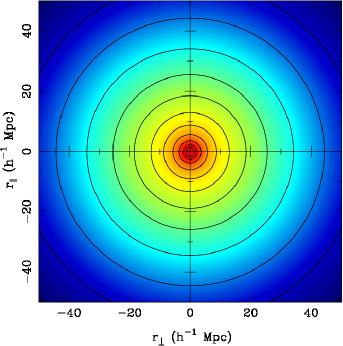
(a) Real space

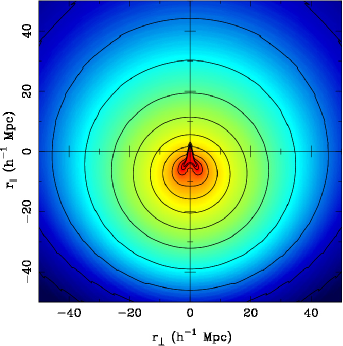
(b) With grav. redshifts $\times 500$

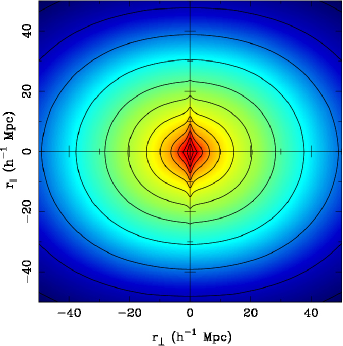
(c) With pec. vels.

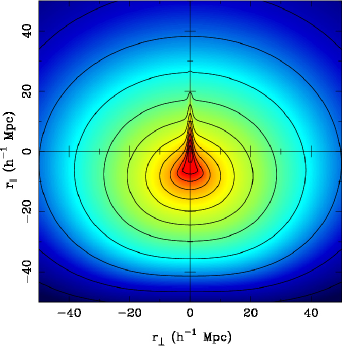
(d) With grav. redshifts $\times 500$ and pec. vels.

Figure 1: Redshift distortions of the cross-correlation function of two populations of galaxies (high and low mass), using a halo model of galaxy clustering (Section 2). We show the effect of peculiar velocities and gravitational redshifts separately (top right and bottom left panel respectively) and together (bottom right). The magnitude of the gravitational redshift component has been magnified by a factor of $500$ in order to make its effect easily visible.

For $\xi_{g1\rho}$ and $\xi_{g2\rho}$ we use a fit inspired by the fact that clustering of galaxies and dark matter can be described by terms which are a combination of internal halo structure and large-scale, linear clustering (the halo model see e.g., Sheth and Cooray 2002 for a review). We use

$$\xi_{g\rho}(r)=\rho_{0}\left[\frac{r}{R_{s}}(1+\frac{r}{R_{s}})^{2}\right]^{-1}+b\xi_{\rm CDM}(r),$$ (4)

where we assume that the internal galaxy halo structure follows the Navarro et al. (1997) relation ($\rho_{0}$ and $R_{s}$ are free parameters) and $\xi_{\rm CDM}$ is the linear theory Cold Dark Matter correlation function (computed using Lewis & Challinor, 2011). Here $b$ is a linear bias parameter relating galaxy and matter clustering on large scales and is a monotonically increasing function of galaxy mass (see e.g. Mo and White 1996).

Having computed $z_{g}(r)$ we use it to distort the cross-correlation function of $g1$ and $g2$ galaxies in redshift space, $\xi_{g1g2}(s_{\perp},s_{\parallel})$. Here $s_{\perp}$ and $s_{\parallel}$ are respectively the distance between pairs of $g1$ and $g2$ galaxies perpendicular and parallel to the line of sight, and $s_{\parallel}$ can be either positive or negative.

There is also the additional distortion of $\xi_{g1g2}(s_{\perp},s_{\parallel})$ due to peculiar velocities. As in Croft et al. (1999), we model this using a spherical infall model for large scale flows (taken from Yahil 1985) and a small scale random velocity dispersion (e.g., Davis and Peebles 1983). The infall model is

$$v_{\rm infall}(r)=-\frac{1}{3}\Omega_{0}^{0.6}H_{0}r\frac{\delta(r)}{[1+\delta(r)]^{0.25}}$$ (5)

where $\delta(r)$ is the matter overdensity averaged within radius $r$ of $g1$ galaxies:

$$\delta(r)=\frac{3}{r^{3}}\int^{r}_{0}\xi_{g1\rho}(x)x^{2}dx$$ (6)

Croft et al. (1999) found that this velocity field model gives a better match than linear theory for the infall pattern around galaxy clusters. Because here we are interested in the redshift distortions around massive galaxy halos, we expect the model to work well in the current context also. This is borne out in our tests with numerical simulations (Section 3). Because $v_{\rm infall}(r)$ is not expected to describe the virialized regions of clusters, we follow Croft et al. (1999) and truncate $v_{\rm infall}(r)$ on small scales by multiplying by an exponential, $\exp{-(\delta/50)}$.

The random velocity dispersion we use is an exponential model, so that the distribution function of velocities is

$$f(v)=\frac{1}{\sigma_{12}\sqrt{2}}\exp\left(-\frac{\sqrt{2}|v|}{\sigma_{12}}\right),$$ (7)

where $\sigma_{12}$ is the pairwise velocity dispersion of $g1-g2$ pairs of galaxies, which we assume to be independent of pair separation. Based on simulation results we take this value to $\sigma_{12}=400{\rm\;km\;s^{-1}}$.

After applying the infall model, gravitational redshift and convolving with $f(v)$, the redshift space cross-correlation function is therefore:

$$\xi_{g1g2}(r_{\perp},r_{\parallel})=\int^{\infty}_{\infty}dvf(v)\xi_{g1g2,iso}\left(r_{\perp},r_{\parallel}-H_{0}^{-1}(cz_{g}(r)-r_{\parallel}r^{-1}v_{\rm infall}(r)-v)\right),$$ (8)

(valid at redshift $z=0$) where $\xi_{g1g2,iso}$ is the isotropic (real space) cross-correlation function of $g1$ and $g2$ galaxies, which we also model using Equation 4.

To make theoretical predictions for $\xi_{g1g2}$ we fit the free parameters in Equations 4 and 7 ($b$, $\rho_{0}$, $\sigma_{12}$) using simulations (see Section 3). In Figure 1 we show contours of $\xi_{g1g2}(r_{\perp},r_{\parallel})$, illustrating the effects of the different redshift distortions. We use parameters in Equation 4 which are appropriate for halos with mass $>3\times 10^{13}{h^{-1}M_{\odot}}$, where the two populations of galaxies $g1$ and $g2$ are the high and mass low halves of the set of halos.

Because the gravitational redshift is so small, for illustrative purposes we have multiplied $z_{g}$ by a factor of 500 when making Figure 1. This should be borne in mind when assessing the relative effects shown. The top left panel of Figure 1 shows the undistorted, isotropic correlation function (Equation 4). In panel (b) we can see that the effect of gravitational redshifts without peculiar velocities is to shift the contours of $\xi_{g1g2}$ downwards, corresponding to a relative blue shift for the $g2$ galaxies clustered around the $g1$ galaxies. In panel (c) the peculiar velocity distortion has been applied on its own, resulting in a distortion of $\xi_{g1g2}$ which has reflection symmetry about the $r_{\perp}$ axis. The large scale squashing of the contours can be seen (the Kaiser (1987) effect) as well as the small scale elongation of $\xi_{g1g2}$ due to the random velocities.

In panel (d) we show gravitational and peculiar velocity redshift distortions together. We can see that as the effect of Kaiser (1987) infall is to boost the correlation function overall, this will also enhance the strength of the asymmetric signal due to gravitational redshifts. This illustrates that both peculiar velocity and gravitational redshift distortions will need to be modelled together in order to make precise constraints on cosmological theories using $z_{g}(r)$.

Given a set of $g1$-$g2$ galaxy pair separation measurements, one now needs to formulate an estimator of the asymmetry of clustering which can probe $z_{g}(r)$. In the galaxy cluster case (KC04, W11), the pair separations were binned into cylindrical shell bins, which was appropriate because the clusters were being treated as distinct objects. In the current large-scale structure case, we have decided to instead bin the pairs in spherical shell bins, and our statistic sensitive to $z_{g}(r)$ is the mean $r_{\parallel}$ position of the pair-weighted centroid of each shell:

$$z^{\rm shell}_{g}(r^{\prime})=\frac{\int^{r^{\prime}+\Delta r^{\prime}}_{r^{\prime}}Hr_{\parallel}[1+\xi(r_{\perp},r_{\parallel})]r^{2}dr}{\int^{r^{\prime}+\Delta r^{\prime}}_{r^{\prime}}[1+\xi(r_{\perp},r_{\parallel})]r^{2}dr}$$ (9)

This estimator $z_{g}^{\rm shell}(r)$ will tend to zero at large and small scales. On small scales this is because the $z_{g}^{\rm shell}(r)$ shift cannot be larger than the spherical bin radius. On large scales this is because the clustering tends towards homogeneity and it is not possible to detect a blueshift or redshift of a homogeneous set of particles. We will explore the exact shape of $z^{\rm shell}_{g}(r)$ in Section 3 below. We note that other measures of the asymmetric distortion of the correlation function could be chosen. For example one could bin galaxy pairs not in spherical bins but in bins matched to the expected shape of contours of $\xi_{g1g2}(r_{\perp},r_{\parallel})$. Or else one could imagine carrying out a full fit to the observed $\xi_{g1g2}(r_{\perp},r_{\parallel}$ data varying parameters in our theoretical model. In the present paper we restrict ourselves to the simple estimator of distortion in Equation 9 and leave exploration of possibly more sensitive measures of $z_{g}(r)$ to future work.

3 Simulation tests

We now compare the results of the theoretical predictions for the $z_{g}$ distortion of Section 2 to results from numerical simulations. It should be borne in mind that both the galaxy-mass cross-correlation function and the $g1$-$g2$ galaxy cross-correlation function enter into the predictions for the observable quantity (Equation 9 ) and so to make predictions we will make some simplifying assumptions about galaxy formation. Here we will associate galaxies with dark matter subhalos and assume that applying a dark matter mass cut to a subhalo population is equivalent to applying a luminosity cut to galaxies.

3.1 Simulations and galaxies

We have used the P-Gadget (see Springel 2001,2005, Khandai et al. 2011) N-body code to run 10 realizations of a $\Lambda$CDM universe. The cosmological parameters used were : amplitude of mass fluctuations, $\sigma_{8}=0.8$, spectra index, $n_{s}=0.96$, cosmological constant parameter $\Omega_{\Lambda}=0.74$, and mass density parameter $\Omega_{m}=0.26$. The cubic periodic box side length was $1\;h^{-1}{\rm Gpc}$, and the number of particles $768^{3}$ per realization, leading to a particle mass of $1.5\times 10^{11}{h^{-1}M_{\odot}}$. The gravitational force resolution was $20h^{-1}{\rm kpc}$, so that subhalo structure is not well resolved (we return to this below).

The bound structure finder SUBFIND (Springel 2001) was used to find galaxy sized subhalos. Because the current relevant redshift surveys (e.g., BOSS, Ahn et al. 2012) are focussed on massive galaxies, we make two different subhalo samples, one where subhalos are above a mass limit of $10^{13}{h^{-1}M_{\odot}}$ (64 particles) and the other above $3\times 10^{13}{h^{-1}M_{\odot}}$.

We compute the gravitational redshift $z_{g}$ of the central particle in each subhalo, and assign that to be the $z_{g}$ associated with the galaxy inside the subhalo. We have also tried averaging the gravitational redshifts of all particles inside each subhalo instead. We find that while this makes a small difference to the individual $z_{g}$ values it does lead to problems with the pairwise differences between satellite and central galaxies. This is because while the central part of a central subhalo may be in a deeper potential well than nearby satellites, averaging particle $z_{g}$ values over the entirety of the dark matter subhalo decreases the redshift and can often lead to a blueshift with respect to nearby small satellites. This would not happen observationally as the stellar parts of galaxies are more centrally concentrated than the dark matter. We therefore account for this by using only the central particle to assign $z_{g}$ to the galaxy.

As the gravitational potential is very smooth, the distribution of gravitational redshifts of galaxies will be also. It is instructive to plot a slice through the simulation to see the nature of the $z_{g}$ fluctuations which we will be characterising. We have done this in Figure 2, where we show $z_{g}$ on a colour scale with galaxy mass denoted by symbol size. We can see that the most massive galaxies are the most clustered, as expected, and also that the galaxies in the deepest potential well (visible near the center of the slice) are also the most massive. The length scale of the visible $z_{g}$ fluctuations is extremely large, with the main potential well covering most of the $\;h^{-1}{\rm Gpc}$ volume. We will be seeking to measure this structure by measuring $z_{g}$ differences between pairs of galaxies on scales up to 100 $\;h^{-1}{\rm Mpc}$. On average the most massive galaxies will tend to be more clustered and have more positive redshifts (red in Figure 2) and this is what we will measure through the effect of this small shift relative to the nearby lower mass galaxies.

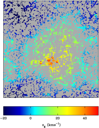
Figure 2: Gravitational redshifts of dark matter subhalos in a simulation. We show a 10 $\;h^{-1}{\rm Mpc}$ thick slice through a $1\;h^{-1}{\rm Gpc}$ N-body simulation cube at redshift $z=0$. Dark matter subhalos are shown with symbol size proportional to (mass)^1/3 and color that indicates their gravitational redshift (positive numbers for redshift). In this case the redshift is not relative to infinity but instead relative to the mean level in the Universe.

After making a galaxy catalogue from a simulation with positions, peculiar velocities and gravitational redshifts defined as above, we apply a mass cut to split it into two halves $g1$ and $g2$ containing an equal number of galaxies. For the $M>3\times 10^{13}{h^{-1}M_{\odot}}$ sample, for which there are an average of $10^{5}$ galaxies in each cubic $\;h^{-1}{\rm Gpc}$, the mass threshold which does this is $5.1\times 10^{13}{h^{-1}M_{\odot}}$. In this case, the mean mass of the low mass half ($g1$) is $3.8\times 10^{13}{h^{-1}M_{\odot}}$ and of the high mass half ($g2$) $1.2\times 10^{14}{h^{-1}M_{\odot}}$. For the $M>3\times 10^{13}{h^{-1}M_{\odot}}$ sample a mass threshold of $1.8\times 10^{13}{h^{-1}M_{\odot}}$ split the sample into two halves, of mean mass $1.3\times 10^{13}{h^{-1}M_{\odot}}$ and $5.6\times 10^{13}{h^{-1}M_{\odot}}$. We note that defining the $g1$ and $g2$ galaxies to be equal halves of a sample may not be the optimal split to get a measurement of gravitaional redshift distortions. For example, in the galaxy cluster (e.g., W11) case the $g1$ galaxies were all the non-BCG galaxies and so comprised most of the sample.

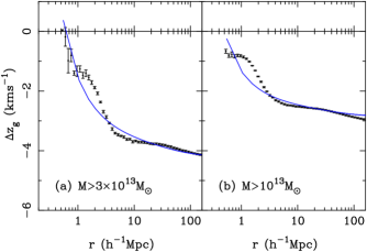
Figure 3: Mean averaged gravitational redshift difference $\Delta z_{g}$ between pairs of dark matter subhalos as a function of separation. In each panel, the lower limit for the mass of subhalos in the sample is given. For each panel, the sample was split into two by mass (high and low mass halves) and $\Delta z_{g}$ was computed from mean difference in gravitational redshifts for galaxies in the two samples as a function of pair separation. Results for simulations are shown by points with error bars. The solid curves show results computed by integrating a simple analytic fit to the subhalo-mass cross-correlation function (see Equation 4)

3.2 Pairwise $z_{g}(r)$ from simulations

In the simulations, the gravitational redshift of each galaxy is available, so that one can directly compute the mean $z_{g}$ difference between pairs of $g1$ and $g2$ galaxies as a function of pair separation. While this would not be available observationally, it is a useful first test of the prediction for $z_{g}$ from Equation 2. For all pairs of $g1$ and $g2$ galaxies in the simulation we compute the redshift difference $\Delta z_{g}=z_{g,g2}-z_{g,g1}$ and bin the results as a function of pair separation. We show the results in Figure 3, as points, with error bars derived from the standard deviation among the 10 simulation realizations. We also show the predictions made using Equation 2 as a smooth line. On small scales $r\lower 2.15277pt\hbox{$\;\buildrel<\over{\sim}\;$}0.5\;h^{-1}{\rm Mpc}$, the theoretical predictions are relatively sensitive to the internal structure of subhalos, in a regime which is not well resolved in the simulations. To deal with this, when integrating Equation 4 we introduce a free parameter $r_{\rm cut}$ so that $\xi_{g\rho}(r)=\xi_{g\rho}(r_{\rm cut})$ for $r<r_{\rm cut}$, and we adjuste $r_{\rm cut}$ so that the simulation and theoretical results in Figure 3 match at the small scale end.

As expected, the $g2$ galaxies have a relative blueshift, and this increases as a function of distance from the $g1$ galaxy, reaching $\sim 4{\rm\;km\;s^{-1}}$ at $100\;h^{-1}{\rm Mpc}$ in panel (a) (galaxies above mass $3\times 10^{13}{h^{-1}M_{\odot}}$ and $\sim 3{\rm\;km\;s^{-1}}$ for panel (b), the lower mass galaxy catalogue. There is a knee in the $\Delta z_{g}$ curves at $r\sim 2-3\;h^{-1}{\rm Mpc}$, related to the transition in $\xi_{g\rho}$ between the regime internal to subhalos and large scale linear cross-correlation function. The theoretical predictions broadly follow the simulation results, although there are kinks in the simulation trend at smaller scales. Future work with higher resolution simulations will be needed to investigate how well the halo model prediction can be made to fit on these scales. In the present case, we will see in Section 3.3 that some information on these scales is washed out by peculiar velocity distortions in any case.

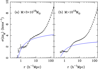
Figure 4: $\sigma(\Delta z_{g})$, the dispersion about mean averaged gravitational redshift difference $\Delta z_{g}$ plotted in Figure 3. We again give in each panel the lower limit for the mass of halos in the sample. Results for simulations are shown by points with error bars. The solid curves not a theoretical prediction for this quantity, but instead are the theory curves for $z_{g}$ from Figure 3 to aid comparison of the two plots.

Equation 2 deals with averaged mass and gravitational redshift profile around galaxies. There will however be galaxy to galaxy variation of this quantity, and this will lead to a dispersion in gravitational redshifts as a function of scale. Because this dispersion will be symmetric about $r_{\parallel}=0$, in observational data it will be completely hidden by the much larger symmetric signal due to the dispersion in peculiar velocities and so unobservable. It is nevertheless instructive to measure the dispersion about the mean $\Delta z_{g}$ profile in simulations. One reason for this is that in Section 4 we will make mock catalogues where model the signal from a much larger number of galaxies by boosting $z_{g}$. This will also amplify the contribution of the dispersion in $\Delta z_{g}$ so that we need to understand its magnitude.

The results for the dispersion about $\Delta z_{g}(r)$, $\sigma(\Delta z_{g}(r))$ are shown in Figure 4. We have also plotted the theory curves for $\Delta z_{g}(r)$ from Figure 3 (we have no theoretical prediction for $\sigma(\Delta z_{g}(r))$ to guide the eye. We can see that the dispersion about the mean profile is approximately equal to the mean profile until about $\sim 2-5\;h^{-1}{\rm Mpc}$ and after this it rises relatively steeply until it is of the order of $\sim 10{\rm\;km\;s^{-1}}$ at $r=100\;h^{-1}{\rm Mpc}$. It is still much smaller than the random redshift dispersion from peculiar velocities, however (which is $\sim 400{\rm\;km\;s^{-1}}$).

3.3 Gravitational redshift estimator

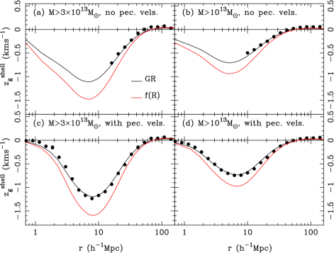
Figure 5: The gravitational redshift estimator $z^{\rm shell}_{g}(r)$ (see Equation 9) plotted as a function of shell radius $r$. We show results measured from simulations as points (with error bars derived from the scatter between 10 realizations). The solid lines show the halo model inspired predictions of Equations 2 and 9, for both general relativity (black line) and the f(R) model of Section 2. The top panels show results with no peculiar velocities added to galaxy redshifts and the bottom panels show the results including all terms in Equation 1 and represent the observable quantity. The left and right panels show results for samples of subhalos with different lower mass limits (given in the legend).

Having seen that the intrinsic pairwise gravitational redshift differences between galaxies in simulations can be modelled, we now turn to the estimator $z_{g}^{\rm shell}(r)$ of Equation 9 which can be applied to observational data. Applying the estimator to simulation data in a periodic volume with a uniform selection function is equivalent to finding the centroid of shells containing pairs of galaxies at different separations. In observational data a random catalogue would need to be used to account for the uniform survey coverage, volume of bins and so on.

We would like to show a comparison between simulation and theory for the $z_{g}^{\rm shell}(r)$ statistic. One issue is that the $z_{g}$ component of the redshift is extremely small, compared to the other redshift components, so that averaging over an extremely large number of simulated galaxies is needed to give a comparison with good signal to noise. Rather than running hundreds more simulations, we instead choose to boost the contribution of the $z_{g}$ component by multiplying it by a large factor (as was done to make Figure 1). When computing the theoretical prediction from Equation 8 we can also multiply $z_{g}$ by the same factor (we use a factor of 100 here) and therefore make a consistent comparison. We then divide the final results by this factor in order to plot the $z_{g}$ curves with the amplitude they would have had without boosting them (therefore only the relative contribution of the noise has been changed).

In Figure 5, we show $z_{g}^{\rm shell}(r)$ for the simulations as points and theoretical predictions as lines, for both galaxy catalogues. We show the results separately without and with peculiar velocities (top and bottom panels respectively). When showing the results without peculiar velocities, the simulations include the dispersion about the mean $z_{g}$ profile plotted in Figure 4 whereas the theory does not model this. Because boosting the $z_{g}$ values in the simulation by a large factor to make the signal to noise low also boosts the dispersion $\sigma(\Delta(z_{g})$, this means that comparison with the theory curves is not possible on small scales. We can see that the theory curves track the large scale simulation plots that are plotted well.

The shape of the curves in Figure 5 shows the blueshift of galaxies surrounding more massive ones, which produces a larger and larger asymmetry in the centroid shift of shells until between 6-9 $\;h^{-1}{\rm Mpc}$ when the signal decreases. The exact point where this happens will depend on the shape of the galaxy-mass cross-correlation function. As the large scale galaxy density field becomes more uniform on large-scales, this shell centroid blue shift becomes smaller. On largest-scales ($r>50-60\;h^{-1}{\rm Mpc}$), the shell centroid actually becomes slightly redshifted with respected to the central galaxy.

In the bottom panel of Figure 5 we show the results in redshift space, where we can see that because the peculiar velocities are dominant in smoothing out the correlation function on small scales that the theory and simulations agree reasonably well there also. This is obviously the situation which will apply when dealing with observations, and so any remaining differences on small scales between theory and simulations will be due to a combination of differences in the gravitational redshift profile (Figure 3) and the peculiar velocity modelling.

If we compare the top and bottom panels of Figure 5, we can see that the effect of peculiar velocities is to slightly increase the signal on scales $r>5\;h^{-1}{\rm Mpc}$. It can be seen that the maximum blueshift of $g2$ galaxies in shells around $g1$ galaxies is around $1{\rm\;km\;s^{-1}}$. This is signficantly less than the blueshifts of up to $14{\rm\;km\;s^{-1}}$ seen by W11, and shows that by splitting the galaxies into equal halves (of $g1$ and $g2$ galaxies) we make the signal numerically much smaller than the redshift profile around rarer galaxies at the centers of massive clusters. The number of pairs of galaxies is obviously maximized by our choice, but the signal to noise of the $z_{g}$ measurement may not be. We leave the question of how best to partition a galaxy sample to make cross-correlations and also the best $z_{g}$ estimator to use to future work.

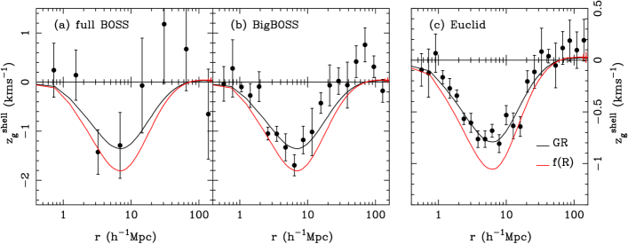
Figure 6: The points show $z_{g}$ measured by observing mock catalogs made from simulations. The error bars were computed from the standard deviation of the measurement from 10 subsamples in each case. We show predictions for the full BOSS survey, BigBOSS and Euclid galaxy redshift surveys. The lines are the predictions of Section 2 which used a halo model fit to the halo-matter cross-correlation function. The black curve shows the prediction of General Relativity and the red curve the simple estimate of an $f(R)$ gravity model mentioned in Section 2.

4 Mock catalogues

In order to make some approximate predictions for results that can be expected by measuring $z_{g}^{\rm shell}(r)$ from current and upcoming large redshift surveys, we have made some very simple mock catalogues from our simulations. The three galaxy redshift surveys which we deal with are
(a) the full SDSS/BOSS galaxy survey (Aihara et al. 2011, Eisenstein et al. 2011) which will be complete in 2014 and will contain $1.5\times 10^{6}$ Luminous Red Galaxies (LRGs) below redshift $z=0.7$.
(b) the BigBOSS galaxy redshift survey (Schlegel et al. 2009) which will measure redshifts for $15\times 10^{6}$ Emission Line Galaxies (ELGs) between redshifts $z=1$ and $z=2$ and $3.5\times 10^{6}$ LRGs between redshifts $z=0.2$ and $z=1.0$. The survey us expected to begin in 2017 and finish in 2022
(c) the Euclid spectroscopic survey (Laureijs et al. 2011) which will use space-based slitless spectroscopy to measure redshifts for between $50-80\times 10^{6}$ ELGs from $z=0.5$ to $z=2.0$. The expected launch date for Euclid is 2020.

As M09 has pointed out, the measurement of $z_{g}$ from the cross-correlation of two populations of galaxies is limited only by shot noise and not by cosmic variance. This is the same property which enables peculiar velocity redshift distortions to be measured limited only by shot noise (McDonald & Seljak 2009). Therefore the signal to noise of a $z_{g}$ measurement in a survey of volume $V$ containing $N_{\rm survey}=\overline{n}V$ galaxies, scales as $V^{1/2}$, and also as $\overline{n}^{1/2}$ as these quantities are changed (M09). As a result when making predictions, to first order the number of galaxies $N_{\rm survey}$ is the important quantity and it is a reasonable approximation to scale our simulations by a factor to account for the differing shot noise resulting from the different numbers of galaxies in each survey. Although we have $N$-body simulations for only 10 $(1\;h^{-1}{\rm Gpc})^{3}$ volumes, with a maximum $4\times 10^{5}$ galaxies of mass $>10^{13}{h^{-1}M_{\odot}}$ per volume, this scaling to account for the number of galaxies allows us to make predictions for surveys containing many more galaxies.

Other simplifications which we make here are to make the $z-$axis of the simulation boxes be the line-of-sight (the plane-parallel approximation), rather than modelling any actual survey geometrical effects. We also carry out all measurements at a single redshift $z=0$ (in practice there will also be a dependence on the mean redshift of the survey e.g., the perturbation growth factor at $z=1$ is 0.62 for the standard cosmology so perturbations in the gravitational potential will be $38\%$ smaller). We use the galaxy catalogue with mass limit $m>3\times 10^{13}{h^{-1}M_{\odot}}$ to model surveys (a) and (b) and the mass limit $m>10^{13}{h^{-1}M_{\odot}}$ to model survey (c). For survey (b) we have also not modelled the ELG and LRG populations separately, but only include in our mock the $15\times 10^{6}$ ELGs. We also do not include other asymmetric distortion terms in the correlation function, such as Transverse Doppler effect (we discuss them in Section 5.2 below). We leave more sophisticated modelling of observational predictions to future work. Our aim here is to make a rough assessment of the detectability of $z_{g}$ signals from large-scale clustering.

When making mock surveys (a)-(c) we therefore scale the gravitational redshift $z_{g}$ for galaxies to account for differing shot noise values. The scaling factor which we multiply by is $s=\frac{\sqrt{N_{\rm survey}}}{\sqrt{N_{sim}}}$ where $\sqrt{N_{sim}}$ is the number of galaxies in all realizations of the simulations added together ($10^{6}$ for the $3\times 10^{13}{h^{-1}M_{\odot}}$ mass limit and $4\times 10^{6}$ for the $10^{13}{h^{-1}M_{\odot}}$ mass limit). We take $N_{\rm survey}$ to be $1.5\times 10^{6}$ for full BOSS, $15\times 10^{6}$ for BigBOSS and $80\times 10^{6}$ for Euclid.

In Figure 4 we show the results measured from these mock catalogues. The error bars show the error on the mean computed from the standard deviation of 10 subsamples (the 10 simulation realizations). We can see that the relative blueshift as a function of scale should be detectable in the full BOSS survey. The difference in chi-squared from zero is 16, indicating a 4 $\sigma$ detection. We have assumed a diagonal covariance matrix however. Future work should use a larger number of simulations to be able to compute and include the off diagonal terms.

The BigBOSS and Euclid surveys should also enable the shape of the curve as a function of scale to be traced out, with information on $z_{g}$ up a few tens of $\;h^{-1}{\rm Mpc}$ being accessible. The overall amplitude of the curves is measurable to $6.5\%$ precision for BigBOSS and $4.0\%$ for Euclid.

5 Summary and Discussion

5.1 Summary

Using the halo model, we have made predictions for the relative gravitational redshifts between pairs of galaxies above and below a mass threshold as a function of scale. We have shown how this relates to distortions in the galaxy cross-correlation function. Comparing this to measurements from observational data should enable constraints to be made on gravity models on large scales. In our theoretical and simulation study we have found that

(1) The large-scale relative gravitational redshifts between simulated galaxies can be predicted well from the halo model. On small scales, internal to galaxy halos our comparison is hampered by limited simulation resolution but still gives good enough predictions for the observable quantity [(2), below].

(2) The gravitational redshifts distort the galaxy cross-correlation function so that it is asymmetric about the $r_{\perp}$ axis. When this asymmetry is quantified by measuring the pair-weighted centroid shift of spherical shells it peaks at a pair separation of $\sim 6-9\;h^{-1}{\rm Mpc}$.

(3) Peculiar velocities smooth out the correlation function in redshift space. This has the advantage that after this smoothing the small scale clustering which is most difficult to predict does not have to be known so accurately. It also has the disadvantage that peculiar velocity modelling will form a necessary part of accurate interpretation of gravitational redshifts.

(4) Current galaxy redshift surveys such as SDSS/BOSS should be able to detect large scale gravitational redshifts from the distortion of the correlation function. Future larger surveys such as BigBOSS and Euclid should be able to make measurements of the distortion out to tens of $\;h^{-1}{\rm Mpc}$ scales with a precision good enough to differentiate between some alternatives to General Relativity.

5.2 Discussion

The measurement of gravitational redshifts of galaxies, starting with W11 has effectively opened a new window on the distribution of matter in the Universe and its gravitational effects, complementary to weak lensing and redshift distortion measurements, but with many different dependencies on survey geometry, model parameters and underlying physics.

Although larger samples of galaxies are required to reach results, gravitational redshifts have several potential advantages over competing probes such as gravitational lensing or peculiar velocities (see also M09). For example, lensing effectively gives a constraint on the projected mass density (the lensing kernel is broad in redshift), whereas gravitational redshifts are localized in 3D space. Redshifts also give a constraint on the potential at one instant in time, rather than an integral over time which is the case for redshift distortions from peculiar velocities.

The measurement of $z_{g}$ from large-scale structure and also the combination of those results with measurements from galaxy clusters will enable constraints to be put on cosmological models (for example the amplitude of the signal in Figure 4 will scale with the amplitude of mass fluctuations, $\sigma_{8}$). By the same token, the dark matter can be probed, for example by examining the difference in the predicted profile of galaxy clusters with and without massive neutrinos. In order to constrain modified gravity scenarios, it will be necessary to combine the data with other measures of the gravitating matter, for example through redshift distortions. This was done by W11 on cluster scales. On large scales, weak lensing and Kaiser (1987) infall have been used by Reyes et al. 2010 to make such constraints.

We note that the calculation of the observability of $z_{g}$ effects in large-scale clustering by M09 results in significantly more pessimistic conclusions than ours (M09 estimates $3-5\sigma$ detectability from a Euclid-scale experiment). However, W11 detected gravitational redshifts at just under $3\sigma$ significance with only of order $10^{5}$ cluster galaxies. This indicates that the inclusion of non-linear scale clustering, (which we have shown can be modelled well in principle) can dramatically increase the chances of making a precise measurement. As an example of this, we have tried recomputing the curves shown in Figure 5 but including only the linear CDM correlation function term in Equation 4. In this case, we find that the curves on scales $r>20\;h^{-1}{\rm Mpc}$ in Figure 5 are similar to the full Equation 4 case, as expected (large-scale clustering is not affected). However on smaller scales the relative blueshift is reduced by a factor of at least 20 indicating that non-linear clustering and halo structure are both important to the success of $z_{g}$ measurements.

We have mentioned in Section 1 that several effects other than $z_{g}$ can cause asymmetries in measured galaxy correlation function. With these effects, one can either decide that they represent further opportunities to probe physics on large scales, or one can decide to model and marginalise over them. M09 has shown for example that when using Equation 1 the true value of $H(z)$ is not known, only the observed redshift of the galaxy. The same is true of the growth parameter determining density fluctuation amplitude. These and similar issues lead to terms appearing in the prediction for galaxy clustering which have been calculated in the context of General Relativity by Yoo et al. (2009,2011). M09 showed that these terms appear at the same order in wavenumber $k$ as $z_{g}$ terms in the imaginary part of the cross-spectrum. The calculation of these terms relies on perturbation theory and their amplitude on the $k\sim 1\;h\;{\rm Mpc}^{-1}$ scales most relevant to the non-linear signal discussed in this paper is likely to be small, but should be investigated in future work.

Related to this, we remind the reader that we have only used the plane parallel approximation in our simulations and mock catalogues, as well as neglecting evolution across the simulation volume. As K13 has explained, geometrical and other effects can lead to asymmetries in clustering in redshift space and these terms need to be dealt with. Around galaxy clusters, the precise magnitude of geometrical effect is related to how galaxies at large distances join the Hubble flow. K13 has shown that this can be large at large impact parameters and will need to be understood and modelled well. For example, when dealing with observational data, extremely finely sampled random catalogs should be made to ensure that the volume-weighted centroid of shells around galaxies is used to compute the statistic plotted in Figure 4.

Evolution of clustering will lead to asymmetries because the overall clustering amplitude on the higher redshift side of each galaxy will be lower than on the lower redshift side. This will lead to asymmetries in the correlation function. These terms are addressed in linear theory by M09 and Yoo et al. (2009) and in the context of inflow of galaxies into clusters by K13.

In the virialized regime of clusters, other new terms become relatively important. For example, Zhao et al. (2012) have shown that the Transverse Doppler effect mentioned in Section 1 is generically present alongside gravitational redshift because the virial theorem relates the potential to the kinetic energy of galaxies. In galaxy cluster models inspired by the data and measurements of W11, Zhao et al. (2012) find that the Transverse Doppler effect (of opposite sign to $z_{g}$) dominates over $z_{g}$ within the inner $\sim 0.2\;h^{-1}{\rm Mpc}$ of clusters. At radii $r>3\;h^{-1}{\rm Mpc}$, the contribution drops to $<5\%$ of $z_{g}$ and so it will be relatively unimportant over most of the scales considered in this paper.

Also important in clusters is the Doppler beaming effect (K13) which causes galaxies moving towards the observer to have a higher surface brightness and hence luminosity. This causes the number of galaxies above a flux limit to vary and again causes an asymmetry of galaxy density around clusters. K13 has shown in the case of W11, the flux limit lies at the steep end of the galaxy luminosity function, so that small changes in flux have large effects on the number of galaxies included in the catalogue. The Doppler beaming effect has the same sign as $z_{g}$ and K13 find that it is the next most important effect after $z_{g}$ for the W11 parameters. It also falls off as a fraction of $z_{g}$ at larger radii.

Apart from general and special relativistic, geometry, and clustering evolution effects on the symmetry of clustering, one can imagine other uncertainties such as dust extinction (less galaxies seen behind a galaxy than in front), or lensing magnification (usually causing the opposite effect, e.g., Hui et al. 2007). Fang et al. (2011) have examined the effect of the former on anisotropies in galaxy clustering and find that its effect is largest on large scales and along the line of sight. Incomplete knowlege of galaxy formation can also lead to uncertainty, as for example in a realistic observational case we would need to choose which galaxies to put into high and low mass subsamples using their luminosities. Also, when comparing with predictions from modified gravity models, the difference between large scale mass distributions inferred from dynamics (peculiar velocity distortions on) and from gravitational redshifts will necessitate some treatment of how galaxies trace mass.

Galaxy redshift surveys are not the only datasets which could be used to probe the large scale gravitational potential with gravitational redshifts. For example, Broadhurst et al. 2000 proposed that with high resolution X-ray spectroscopy, intracluster gas could be used to map out $z_{g}$ in large galaxy clusters. More relevant to the large-scale structure case are 21cm neutral hydrogen surveys (e.g., Peterson & Suarez 2012). As M09 has pointed out, the 21cm flux field could form a good contrast to the highly clustered field probed by bright galaxies and as $z_{g}$ measurements are differential could lead to better measurements. In this case, the formalism which we have outlined in this paper should make it possible to start modelling the range of scales and densities required.

The current and upcoming generations of large cosmological surveys will contain enough data that qualitatively new effects such as gravitational redshift distortions to clustering can be looked for. With only two published detections so far, galaxy gravitational redshifts are perhaps two decades behind weak lensing as a field. Unlike lensing in the early 1990s, however, surveys two orders of magnitude larger than those currently analysed are already planned for other purposes. These have the promise to bring gravitational redshifts into the precision cosmology era.

References

- [] Ahn, C.P. et al. , 2012, ApJS, 203, 21
- [] Aihara, H. et al. 2011, ApJS, 193, 29
- [] Broadhurst, T. and Scannapieco, E., 2000, ApJL, 533, 93
- [] Cappi, A., 1995, A& A, 301, 6
- [] Chang, T.-C., Pen, U.-L., Bandura, K. & Peterson J.B., 2010, Nature, 466, 463.
- [] Cooray, A., & Sheth, R., 2002, Phys. Rep., 372, 1
- [] Croft, R.A.C., Dalton, G.B.,& Efstathiou, G.P., 1999, MNRAS, 305, 547
- [] Davis, M., & Peebles, P.J.E., 1983, ApJ, 267, 465
- [] Domínguez Romero, M., Lambas, D., Muriel, H., 2012, MNRAS, tmpL.543D, arXiv:1208.3471
- [] Eisenstein, D.,J., et al. 2011, AJ, 142, 72
- [] Fang, W., Hui, L., Menard, B., May, M., Scranton,R., 2011, Phys Rev D, 84, 063012
- [] Greenstein, J. L., Oke, J. B.& Shipman, H. L., 1971, 169, 563
- [] Hirata, C.M., Ho, S., Padmanabhan, N., Seljak, U., & Bahcall, N.A., 2008, PRD, 78, 3520
- [] Ho., S, Hirata, C., Padmanabhan, N., Seljak, U. and Bahcall, N., 2008, PRD, 78, 3519
- [] Hui, L., Gaztañaga, E., & Loverde, M., 2007, Phys. Rev. D, 76, 103502
- [] Kaiser, N. 1987, MNRAS, 227, 1
- [] Kaiser, N. 2013, MNRAS, submitted, arXiv:1303.3663 (K13)
- [] Kim, Y.-R. & Croft, R.A.C., 2004, ApJ, 607, 164 (KC04)
- [] Laureijs, R., et al. 2011, ESA Euclid Red Book, arXiv:1110.3193
- [] Lewis, A. and Challinor, A., ”CAMB: Code for Anisotropies in the Microwave Background”, 2012, Astrophysics Source Code Library, ascl:1102.026
- [] Lopresto, J. C., Schrader, C., & Pierce, A. K., 1991, 376, 757
- [] Malone, T.W., 1981, Cognitive Science, 4, 333, 369
- [] McDonald, P., 2009, JCAP, 11, 026 (M09)
- [] McDonald, P. & Seljak, U., 2009, JCAP, 10, 007
- [] Mo, H.J., & White, S.D.M., 1996, MNRAS, 282, 347
- [] Navarro, J. Frenk, C.S., & White, S.D.M., 1997, ApJ, 490, 493
- [] Nottale, L, 1990, Gravitational Lensing, Eds Mellier, Y., Fort, B. & Soucail, G., Lecture Notes in Physics, Berlin Springer Verlag, 360, 29
- [] Peterson, J.B., & Suarez, E., 2012, proceedings of Moriond Cosmology 2012, arXiv:1206.0143
- [] Pound, R.V., & Rebka, G.A., 1959, PRL, 3, 439
- [] Reyes, R., Mandelbaum, R., Hirata, C. & Bahcall, N., 2008, MNRAS, 390, 1157
- [] Reyes, R., Mandelbaum, R., Seljak, U., Baldauf, T., Gunn, J. E., Lombriser, L. & Smith, R. E., 2010, Nature, 464, 256
- [] Ross, N.P., Myers, A., Sheldon, E., Yeche, C., Strauss, M., Bovy, J., Kirkpatrick, J., Richards, G., 2011, ApJ submitted, arXiv:1105.0606
- [] Schlegel, D. J., Bebek, C., Heetderks, H., Ho, S., Lampton, M., Levi, M., Mostek, N., Padmanabhan, Nikhil; Perlmutter, S., Roe, N., Sholl, M., Smoot, G., White, M., Dey, A., Abraham, T., Jannuzi, B., Joyce, D., Liang, M., Merrill, M., Olsen, K., Salim, S., 2009, eprint arXiv:0904.0468
- [] Springel, V., 2001, New Astronomy, 6, 79
- [] Springel, V., 2005, MNRAS, 364, 1105
- [] White, Martin; Blanton, M.; Bolton, A.; Schlegel, D.; Tinker, J.; Berlind, A.; da Costa, L.; Kazin, E.; Lin, Y.-T.; Maia, M.; McBride, C. K.; Padmanabhan, N.; Parejko, J.; Percival, W.; Prada, F.; Ramos, B.; Sheldon, E.; de Simoni, F.; Skibba, R.; Thomas, D.; Wake, D.; Zehavi, I.; Zheng, Z.; Nichol, R.; Schneider, Donald P.; Strauss, Michael A.; Weaver, B. A.; Weinberg, David H., 2011, ApJ, 728, 126
- [] Wojtak, R., Hansen, S. H. & Hjorth, J., 2011, Nature, 477, 567 (W11)
- [] Yahil, A., 1985, N: ESO Workshop on the Virgo Cluster of Galaxies, Garching, West Germany, September 4-7, 1984, Proceedings (A86-37351 17-90). Garching, West Germany, European Southern Observatory, 1985, p. 359-373.
- [] Yoo. J, Fitzpatrick, A.,L., & Zaldarriaga, M., 2009, Phys. Rev. D, 80, 083514
- [] Yoo, J. and Hamaus, N. and Seljak, U. and Zaldarriaga, M., 2012, Phys. Rev. D, 86, 063514
- [] Zhao, H., Peacock, J., and Li, B., 2012, PRL, submitted, arXiv:1206.5032