Coherent control of phase diffusion in a Bosonic Josephson junction by scattering length modulation

Abstract

By means of a temporal-periodic modulation of the $s$-wave scattering length, a procedure to control the evolution of an initial atomic coherent state associated with a Bosonic Josephson junction is presented. The scheme developed has a remarkable advantage of avoiding the quantum collapse of the state due to phase and number diffusion. This kind of control could prove useful for atom interferometry using BECs, where the interactions limit the evolution time stage within the interferometer, and where the modulation can be induced via magnetic Feshbach resonances as recently experimentally demonstrated.

1 Introduction

A fundamental characteristic of Bose-Einstein condensates (BECs) is that they display coherence phenomena in analogy to classical waves, as was observed back in the early experiments, using Young’s double slit [1] and double-well interference settings [2]. The reason being that the order parameter, the macroscopic wave function, is a complex field with certain amplitude and global phase. Since then, the importance of measuring the relative phase between fragments of condensates with high precision has been recognized, and several different schemes for atom interferometry based in BECs have been devised . One important result along this line is the creation of non-classical (entangled) many-body states [4, 5], as is the case of the so called squeezed spin states [6], exploiting in a controlled way the nonlinear nature of the atom interactions. Noteworthy is its application into a new generation of quantum metrology devices performing below the standard quantum limit [7]. However, at the same time, interactions have detrimental effects in the stage of phase accumulation of the interferometer [8], due to a process generally known as “phase diffusion” [9] blurring the final phase readout and consequently reducing the sensitivity of the device. A possible way out of this problem might be given by the management of Feshbach resonances, given the high degree of control achieved for the different experimental parameters involved with BECs physics in optical lattices [10]. In particular the interatomic interaction, characterized principally by the s-wave scattering length $a_{s}$, can have both its sign and strength tuned by means of external magnetic fields, and this has been used extensively in the proper attainment of BECs [11]; in the study of nonlinear excitations of the condensate, for example in the creation of bright solitons, for the setting of attractive interactions [12]; or in the preparation of an almost ideal Bose gas for Anderson localization observation [13], to name but a few. Another interesting possibility that has been considered is the modulation in time of the scattering length. This has proven useful for the control of matter waves, as in the stabilization of bright and dark solitons [14, 15, 16, 17], self-confinement of 2D and 3D BECs without an external trap [18], and also for the prediction of the remarkable Faraday pattern formation in BECs [19, 20]. Recently a new set of experiments have explored this kind of modulation for the generation of turbulence in BECs [21]: as it was observed, the scattering length modulation suppresses the aspect ratio inversion typically observed in the atomic cloud during free expansion - a signature of the turbulent regime where the cloud expands freely with constant aspect ratio.

In this work we further investigate the effects of the scattering length modulation on the quantum dynamics of a BEC trapped in a double well potential. A typical feature of this system is the existence of two distinct phases: Josephson oscillations, where atoms tunnel coherently from one well to the other; and macroscopic self-trapping, where the interaction between the atoms lead to a halt of the coherent tunneling mechanism [22]. It is well known that in a full quantum description, an initial atomic coherent state will show a series of collapse-and-revivals of relative phase and number due to the atomic interactions and the quantized nature of the matter wave field [23]. This is an intrinsic signature of the nonlinear quantum dynamics, which does not appear in semiclassical mean field approaches, such as the evolution through a Gross-Pitaevskii equation. Remarkably, by using the scattering length modulation at certain frequencies, it is possible to control and avoid the loss of quantum coherence that takes place during the collapsing process. We describe how this suppression of collapse occurs and establish a possible connection which might be important for atom interferometry with BECs. In order to better understand the dynamics of the collapse, we derived a Fokker-Planck equation for the Husimi distribution whose evolution can be visualized on the Bloch sphere parameterizing the relative phase and population difference variables into the usual angular variables of a spherical coordinate system. The paper is divided as follows. In Sec. II we present the quantum mechanical model for the two-mode condensate with scattering length modulation and show some typical and relevant states. In Sec. III we discuss the typical collapse and revival of phase and population dynamics present for a static scattering length. In Sec. IV we present the central results concerning the use of dynamical scattering length in the control of coherence of BECs, and finally in Sec. V we present our conclusions.

2 Model

In order to describe in a full quantum mechanical way an interacting Bose gas trapped in a double-well potential $V\left(\mathbf{r}\right)$, at zero temperature, we use the two-mode Bose-Hubbard model [24, 25] characterized by the Hamiltonian ($\hbar\equiv 1$):

$$\hat{H} = -\frac{\Omega}{2}(\hat{a}_{1}^{\dagger}\hat{a}_{2}+\hat{a}_{1}\hat{a}_{2}^{\dagger})+\epsilon\left(\hat{n}_{1}-\hat{n}_{2}\right)+\kappa\left(t\right)\left[\hat{n}_{1}\left(\hat{n}_{1}-1\right)+\hat{n}_{2}\left(\hat{n}_{2}-1\right)\right],$$ (1)

where $\hat{a}_{j}$ and $\hat{a}_{j}^{\dagger}$ are the annihilation and creation operators for particles in the site $j=1,2$, with an associated spatial wave function $\chi_{j}(\mathbf{r})=\langle\mathbf{r}|\chi_{j}\rangle$ with $|\chi_{j}\rangle=\langle\mathbf{r}|\hat{a}_{j}^{\dagger}|\textrm{vac}\rangle$, satisfying the bosonic algebra $[\hat{a}_{j},\hat{a}_{k}^{\dagger}]=\delta_{jk}$, and $\hat{n}_{j}=\hat{a}_{j}^{\dagger}\hat{a}_{j}$ the corresponding number operators. The tunneling frequency or coupling between sites is defined by $\Omega$, the on-site interaction energy between two atoms in a single well is given by $\kappa$, which is proportional to the atomic s-wave scattering length $a_{s}$ (with the usual positive/negative sign convention for repulsive/attractive interaction), and finally $\epsilon$ is a possible energy offset between the wells caused by an additional external potential, which in this work will be considered equal to zero, i.e. a symmetric trap.

As stated in the introduction, we are interested in the case where $a_{s}$ is periodically modulated via a magnetic Feshbach resonance, so it is composed of an static as well as a dynamic part. To see how this can be done, a relation for $a_{s}$ as a function of the magnetic field $B$ obtained by Moerdijk et al. [26] can be used:

$$a_{s}\left(B\right)=a_{\textrm{BG}}\left(1-\frac{\Delta}{B-B_{\infty}}\right),$$ (2)

with $a_{\textrm{BG}}$ the background or off-resonant value of the scattering length, $B_{\infty}$ the position of the resonance where $a_{s}\rightarrow\pm\infty$, and $\Delta$ the resonance width, determined by the condition $B=B_{\infty}+\Delta$ at which there are no interactions ($a_{s}=0$). In the case of a harmonic magnetic field $B\left(t\right)=\bar{B}+\delta B\cos\omega t$, and far from the resonance so $\delta B\ll\left|B_{\infty}-\bar{B}\right|$ , it is obtained at first order in $\delta B$,

$$a\left(t\right)\simeq\bar{a}+\delta a\cos\omega t,$$ (3)

where $\bar{a}=a_{s}(\bar{B})$ and $\delta a=a_{BG}\Delta\delta B/\left(B_{\infty}-\bar{B}\right)^{2}$. With this expression for the scattering length, the on-site interaction parameter will have the form $\kappa(t)=\kappa_{0}(1+\mu\cos\omega t)$, with $\kappa_{0}$ being the static part of the interaction, and $\mu\equiv\bar{a}/\delta a$, the relative amplitude of the modulation.

To give an idea of actual experimental values, consider for instance the work of Pollack et al. [28], where it was used an ultracold gas of ⁷Li atoms, which display a Feshbach resonance at $B_{\infty}\simeq 737$ G. For $\bar{B}=565$ G and $\delta B=14$ G, they obtained an $\bar{a}\simeq 3.0a_{0}$ with an amplitude of modulation $\delta a\simeq 2.3a_{0}$. Other possibilities could be ⁸⁵Rb (with a resonance at $B_{\infty}\simeq 155$ G), for which the scattering length is $\bar{a}\sim 33a_{0}$ around $\bar{B}\sim 165$ G before becoming negative for larger values of $B$, in this case for example, it could be used values of $\delta B\sim 0.2$ G to produce a modulation of about 30%; or ³⁹K (with a resonance at $B_{\infty}\simeq 402$ G), for which $\bar{a}\sim 6a_{0}$ at $\bar{B}\sim 360$ G and negative for $B<350$ G, and the same modulation can be achieved with $\delta B\sim 2$ G [11].

A natural basis for this system is given by the Fock states,

$$\left|n\right\rangle_{1}\otimes\left|N-n\right\rangle_{2}\equiv\left|n\right\rangle=\frac{(\hat{a}_{1}^{\dagger})^{n}(\hat{a}_{2}^{\dagger})^{N-n}}{\sqrt{n!\left(N-n\right)!}}\left|\textrm{vac}\right\rangle,$$ (4)

labeled by $n=0,1,...N,$ the particle number in one of the wells. They are fragmented states in the sense that the bosons occupy two different spatial modes (with the particular exception of the states $\left|0\right\rangle$ and $\left|N\right\rangle$ in which all bosons are in one mode only). This basis expands an $\left(N+1\right)$-dimensional Hilbert space which is easily accessible to numerical calculations. Evidently the total number of particles is conserved as can be seen directly from the Hamiltonian (1), i.e. $\hat{N}=\hat{n}_{1}+\hat{n}_{2}$ is a constant of motion. A general $N$-boson state ket is then written simply as

$$\left|\psi\left(t\right)\right\rangle=\sum_{n=0}^{N}c_{n}\left(t\right)\left|n\right\rangle,$$ (5)

with $\sum_{n}\left|c_{n}\left(t\right)\right|^{2}=1$, the normalization condition for the time-dependent amplitudes. The $\left|n\right\rangle$ states are also commonly known as spin states, since this model is isomorphic with the SU(2) group through the Schwinger pseudospin operators [29]

$$\hat{J}_{x} = \frac{1}{2}(\hat{a}_{1}^{\dagger}\hat{a}_{2}+\hat{a}_{1}\hat{a}_{2}^{\dagger}),$$

$$\hat{J}_{y} = \frac{1}{2i}(\hat{a}_{1}^{\dagger}\hat{a}_{2}-\hat{a}_{1}\hat{a}_{2}^{\dagger}),$$ (6)

$$\hat{J}_{z} = \frac{1}{2}(\hat{n}_{1}-\hat{n}_{2}),$$

with total angular momentum $J=N/2$ and satisfying the SU(2) angular momentum algebra $[\hat{J}_{i},\hat{J}_{j}]=i\epsilon_{ijk}\hat{J}_{k}$. Clearly the $\left|n\right\rangle$ states are eigenstates of the $\hat{J}^{2}$ and $\hat{J}_{z}$ operators, and then our system can be seen in terms of a giant spin system with a dynamics governed by the Hamiltonian

$$\hat{H}=-\Omega\hat{J}_{x}+2\epsilon\hat{J}_{z}+2\kappa\left(t\right)\hat{J}_{z}^{2}.$$ (7)

Note that $\hat{J}_{z}=\hat{n}-N/2$, is exactly the relative number operator, its mean value giving the population imbalance between the wells.

From the Fock states, a useful basis for the analysis of our problem can be defined, given by the called binomial or atomic coherent states, introduced by Arecchi et al. [30]. They are the more general unfragmented states, which means that all the bosons are in the same single-particle mode, $\cos(\theta/2)\left|\chi_{1}\right\rangle+e^{i\varphi}\sin(\theta/2)\left|\chi_{2}\right\rangle$, where $\theta$ and $\varphi$ determine the amplitude and relative phase, respectively, of single modes $\left|\chi_{i}\right\rangle$, $(i=1,2)$. Defining $\hat{b}_{1}^{\dagger}=\cos(\theta/2)\hat{a}_{1}^{\dagger}+e^{i\varphi}\sin(\theta/2)\hat{a}_{2}^{\dagger}$ as the creation operator of a particle in the single particle state the binomial states are defined as

$$\left|\theta,\varphi\right\rangle=\frac{(\hat{b}_{1}^{\dagger})^{N}}{\sqrt{N!}}\left|\textrm{vac}\right\rangle,$$ (8)

or equivalently as

$$\left|\theta,\varphi\right\rangle=\sum_{n=0}^{N}\sqrt{{N}\choose{n}}\cos^{n}(\theta/2)\sin^{N-n}(\theta/2)e^{i(N-n)\varphi}\left|n\right\rangle,$$ (9)

where the binomial expansion was used. It is worth notice the two special cases: $\left|0,\varphi\right\rangle$ and $\left|\pi,\varphi\right\rangle$ ($\varphi$ undefined), corresponding to the $\left|N\right\rangle$ and $\left|0\right\rangle$ states respectively, which are the only Fock-coherent states in this description.

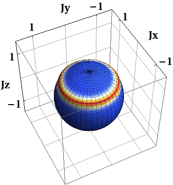
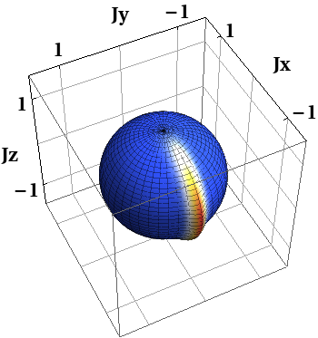
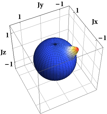
(a)        (b)        (c)

Figure 1: (color online) Examples of Husimi distributions for three different state preparations with $N=100$: (a) Fock state $\left|80\right\rangle$; (b) Phase state $\left|\pi\right\rangle$; (c) Coherent state $\left|\pi/4,5\pi/4\right\rangle$. The $\theta$ and $\varphi$ angles correspond to the usual convention in polar spherical coordinates.

Another basis that can be constructed from the Fock states (4), is given by the Pegg and Barnett relative phase states [31]. This is a useful basis since links the results of BEC interferometry experiments with the two-mode Bose-Hubbard model, providing a way of describing the phase distribution of a particular state. They are defined in terms of the Fock states as

$$\left|\phi_{m}\right\rangle=\frac{1}{\sqrt{N+1}}\sum_{n=0}^{N}\exp(in\phi_{m})\left|n\right\rangle,$$ (10)

with $\phi_{m}=\phi_{0}+2\pi m/(N+1)$, $m=0,1,\ldots,N,$ a quase-continuum angular variable, and $\phi_{0}=-\pi$, so $\phi_{m}\in[-\pi,\pi)$. From this definition is clear that the probability amplitudes $C{}_{\phi}$ of a general state written in this basis: $\left|\psi\left(t\right)\right\rangle=\sum_{n=0}^{N}C{}_{\phi}\left(t\right)\left|\phi_{m}\right\rangle$, are related to the number amplitudes $c_{n}$ via a discrete Fourier transform. (For a thorough discussion about the two-mode formalism see the recent review by Dalton and Ghanbari [25]).

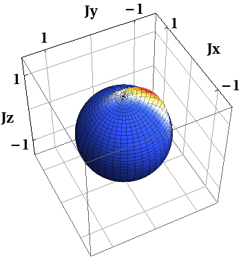
The binomial states (9 ) allow the use of the semiclassical $Q$-Husimi distribution, which is very convenient for visualizing the dynamics of the many-body state on a spherical phase space representation (Bloch sphere), and is given by the quasi-probability distribution of a general state $\left|\psi\right\rangle$ to be in a coherent state (9):

$$Q(\theta,\varphi)=\left|\left\langle\theta,\varphi\left|\psi\right.\right\rangle\right|^{2}.$$ (11)

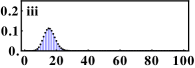
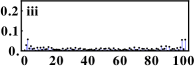
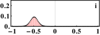
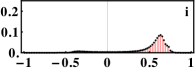
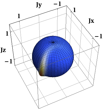
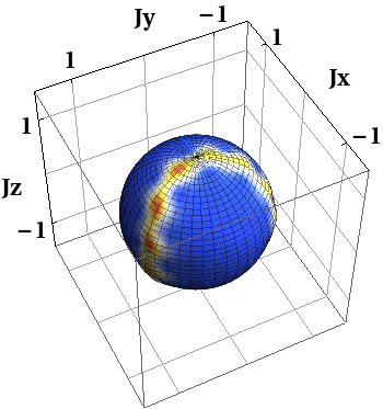
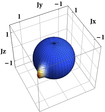
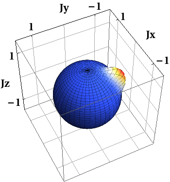
This representation is helpful to interpret the results of a certain dynamics since we can directly extract information about the relative phase and relative number distribution of a particular state. For instance, a Fock state, Fig. 1(a), which has a very definite distribution in relative number has a localized $Q$-distribution along the $z$ axis (which is related to the mean of the $\hat{J}_{z}$ operator); on the other hand, a relative phase state, Fig. 1(b), has a localized distribution around a particular $\phi$ value. Finally, a coherent state, Fig. 1(c), which is the more classical quantum state possible is represented by an equal noise distribution around the central value given by the $(\theta,\phi)$ coordinates in the Bloch sphere.

The numerical results presented in the following two sections were obtained by solving the Schrödinger equation for the Hamiltonian (1) written in the Fock basis (5), yielding a set of $N+1$-coupled differential equations for the expansion amplitudes $c_{n}(t)$. Relative phase information is extracted from the number distribution by taking its discrete Fourier transform.

3 Static scattering length: collapse of the population oscillations

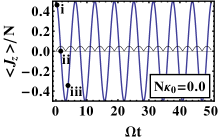
To gain insight into the collapsing process, we start by considering the non-interacting, non-driving case ($\kappa_{0}=0$, $\mu=0$: Rabi regime) in (1) , preparing a system of $N=100$ atoms initially in the Fock state $\left|100\right\rangle$ which corresponds to all bosons located initially in one well, with a $Q$-distribution centered around $\theta=0$, the north pole of the Bloch sphere. As mentioned earlier this is also a coherent state, the relative phase distribution is completely undetermined (uniform distribution) and correspondingly its distribution in relative number is sharp (delta distribution). In this situation, as is well known [32], the boson population performs Rabi oscillations between the wells at the tunneling frequency (Fig 2(a), left). Since the evolution operator is simply $\exp(+i\hat{J}_{x}\Omega t)$, the result of its actuation on a coherent state is to produce another coherent state rotated an angle $\Omega t$ around the $x$-direction in the Bloch sphere, the relative number distribution, Fig. 2(b), changes accordingly going from the delta function at the poles to a Gaussian shape at the equator, with its mean changing in time as $N\cos^{2}(\theta(t)/2)$ and its variance as $N\sin^{2}(\theta(t)/2)\cos^{2}(\theta(t)/2)$, with $\theta(t)=\pi-\Omega t$, as expected for a binomial distribution. The phase distribution in Fig. 2(c) evolves from uniform to binomial distributions centered around $\pm\pi/2$ alternately, as the coherent state goes from west to east of the sphere (since the center of the Husimi distribution always lies on the $yz$-plane), its width changing reciprocally with the width of the number distribution.

(a)

(b)

$\left|c_{n}\right|^{2}$ vs $n$           $\left|c_{n}\right|^{2}$ vs $n$

(c)

$\left|C_{\phi}\right|^{2}$ vs $\phi/\pi$         $\left|C_{\phi}\right|^{2}$ vs $\phi/\pi$

Figure 2: (color online) Comparison of the Rabi ($N\kappa_{0}=0$, left column) and Josephson ($N\kappa_{0}=0.5\Omega$, right column) dynamics, for an initial $\left|N\right\rangle$ Fock state preparation (all $N=100$ bosons in one well) without external driving, illustrating the process of collapse or “diffusion” in relative number. (a) The evolution of the mean relative number $\left\langle\hat{J}_{z}\right\rangle$ (blue thick line) and its standard deviation (black thin line); note how in the Josephson case, the dispersion increases until it reaches a saturation value close to that of a uniform distribution. For the three sample times (i-iii), the relative number (b) and phase (c) distributions are depicted.

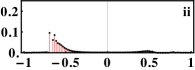
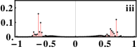
This periodic scenario changes when interactions are taken into account. The evolution operator has now a complicated form since is composed of the tunneling and nonlinear interaction operators, characterized by $\hat{J}_{x}$ and $\hat{J}_{z}^{2}$ respectively, that do not commute, and make it very difficult to evaluate its action analytically in the Josephson regime. When the interactions are not so large compared with the tunneling ($N\kappa_{0}/\Omega<1$), so the boson population is not self-trapped, or equivalently the Husimi distribution is not confined to the poles of the Bloch sphere, the dynamics is still dominated by $\hat{J}_{x}$ but the different Fock states that compose the coherent state will gain a phase $(n-N/2)^{2}$ due to the action of $\hat{J}_{z}^{2}$. This dephasing will cause a spreading in the relative number distribution, its mean tending to zero (a balanced population state) and its variance increasing until it saturates to a value approximately equal to the corresponding to a uniform distribution. This is what is called the collapse of the population oscillations (see the right column of Figs. 2(a) and (b)); it is a direct consequence of the discreteness of the quantum state and is not captured by a mean-field theory which predicts large amplitude anharmonic oscillations between the wells [32]. The phase distribution shows an interesting behavior, since although for short evolution time it shows a well defined distribution, when the relative distribution is smeared out, for later times it tends to a distribution with phase averaged out to zero due to a double-peaked profile as shown at ~$\pm$0.6$\pi$ in Fig. 2(c). We want to note that this process known as “phase diffusion” in the literature, may be a diffusion in relative number (as in this case), relative phase, or even both, depending on the initial state and model parameters, since $\phi$ and $n$ are complementary variables.

(i)        (ii)       (iii)

Figure 3: (color online) Snapshots of the Husimi distribution for three different instants (i-iii) as indicated in fig. 2(a) (right) with the same parameters and initial preparation, showing the collapse of relative population on the phase space.

All those features can be better understood using the Fokker-Planck equation obtained for the evolution of the Husimi distribution, $Q\equiv Q(\theta,\varphi;t)$ (see derivation in the Appendix), which behaves as a nonlinear fluid moving on the spherical Bloch space:

$$\frac{\partial Q(\theta,\varphi;t)}{\partial t} = [-\Omega(\sin\varphi\frac{\partial}{\partial\theta}+\cot\theta\cos\varphi\frac{\partial}{\partial\varphi})$$

$$-2\kappa(N\cos\theta\frac{\partial}{\partial\varphi}-\sin\theta\frac{\partial^{2}}{\partial\theta\partial\varphi})]Q(\theta,\varphi;t).$$

The tunneling term gives rise directly to the orbital angular momentum operator $L_{x}$, thus having the effect of a drifting motion around the $x$ direction, with a drifting coefficient proportional to the tunneling frequency $\Omega$. This term only is the one responsible for the dynamics in the Rabi regime, when no interactions are present ($\kappa=0$). On the other hand, interactions change the whole picture. The interaction term is not translated simply into a $L_{z}^{2}$ operator, since it is produced by a nonlinear operator, yielding two simultaneous effects on the dynamics. One is a drifting motion around the $z$ direction produced by the first term of the second line of Eq. (3), which can be seen is effected by a $L_{z}$ orbital angular momentum operator, with a $\cos\theta$-dependent drifting coefficient, proportional to $N\kappa$; this indicates that the effect of this drifting is stronger near the poles of the sphere and negligible around the equator. The other is a diffusive effect, produced by the cross-derivative in the last term of Eq. (3), with a $\sin\theta$-dependent diffusion coefficient, proportional to $\kappa$ - this term, when positive, spreads the distribution hence being responsible for the loss of coherence, but its strength is much weaker than the drifting motion by a factor equal to the number of particles, which can be very large. Notice that its action is out of phase with the interaction drifting, so the diffusion is more acute in the equator, and also that it depends in both angular variables, as was remarked earlier, for the case of a general diffusion.

In Fig. 3 it is shown how the Husimi distribution evolves under the Fokker-Planck equation (3) in the Josephson regime ($N\kappa_{0}/\Omega<1$), for three sample times, as indicated on the right column of Fig. 2(a) . Since for this set of parameters the tunneling is still dominating, the distribution will rotate around the $x$-direction but now its center will not stay on the $yz$-plane as in the Rabi case due, of course, to the interactions. The latter will cause a twisting around the $z$-axis (drift), and a spreading (diffusion) which generates this strip-like shape. Because the motion depends on the polar coordinate $\theta$, the spreading also occurs in this direction, which causes the loss of definition in relative number. The two peaks of the phase distribution on ~$\pm$0.6$\pi$ in Fig. 2(c) are then understood since the Husimi distribution in this case is well localized in the $\varphi$ direction around these values. If the interaction term were the dominating one ($N\kappa\gg\Omega$: Fock regime), the delocalization in phase space would be in the $\varphi$ direction instead because of the drifting motion around $z$, and then the diffusion would be mostly in relative phase. In this regime, depending on the initial conditions, the slow drifting in the periodic surface around $x$ would cause the distribution to have enough time to accumulate recovering coherence. The exact coordinates of this coherence revival is completely defined by the interplay of the diffusion and drifting mechanisms.

It is interesting to note how the classical transition point where self-trapping starts to appear, is captured naturally from the Fokker-Planck equation (3). Ignoring the diffusion term which is negligible when $N\rightarrow\infty$ (since in this case the mean-field and quantum approaches coincide), and comparing the two remaining terms: the interaction dominates over the tunneling for values of $N\kappa_{0}>\Omega/2$ (In the classical dynamics analysis this is the pitchfork bifurcation point, cf. eq. (47) from Ref. [34] and following discussion).

4 Dynamical scattering length: control of coherence

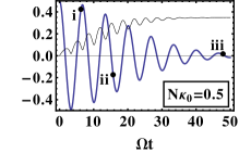
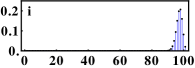
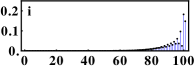
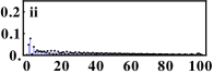
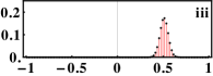
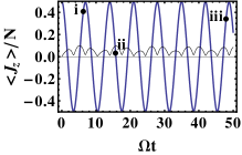
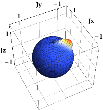
The preceding discussion sets the stage for the main result of this paper, which is to control and utterly avoid the loss of coherence. This occurs when we turn on the driving on the interactions, in a certain region of the modulation parameters (amplitude and frequency), for an initial atomic coherent state in the Josephson regime. In Fig. 4 (top), for example, it is shown the evolution of the mean relative number for the same initial state of Fig. 2, with a driving frequency $\omega=1.8\Omega$ and a modulation amplitude $\mu=0.3$, recalling that the interaction energy has the form $\kappa(t)=\kappa_{0}(1+\mu\cos\omega t)$, as stated in Sec. II. It is remarkable the similarity of this case with the non-interacting (Rabi) regime (c.f. the left column of Fig. 2(a), left), performing complete swapping of boson population without collapsing to a balanced state, only that the period of the oscillations is slightly larger. Also the standard deviation of the relative number operator has the same behavior (black curve), reaching small values when all the bosons are in one of the wells (i.e. the poles of the Bloch sphere in the phase space representation) and its largest values when the population is balanced (equator of the sphere), but keeping always a much lower value than the corresponding to a unifom distribution. Now, in the phase space picture (Fig. 4, bottom), snapshots of the Husimi distribution for different times in the evolution of the system show how the coherence is maintained, since the distribution stays localized, deviating from a coherent state just in that there is a squeezing in the relative phase. It is possible to understand why the distribution keeps its coherence directly from the Fokker-Planck equation. This occurs as the system attains a resonant regime, which depends in a non-trivial manner on $N$, $\Omega$, $\kappa_{0}$, as well as the strength $\mu$ and frequency $\omega$ of the scattering length modulation. In a simplified “averaged” picture in this resonant regime the modulation contributes by changing the diffusion coefficient in a commensurate manner with the drifting around $x$, so that when the diffusion is higher the drifting also is, so there is not “enough time” for the diffusion to induce dephasing of the distribution components, which then keeps coherence. There are fluctuations on this behavior since there is diffusion and also drifting around the $z$-axis, which contribute with this averaged picture to the overall dynamics, but they are small enough in a sense that the state is kept close to a coherent one. We performed numerical tests for a longer time ($\Omega t$~500) than shown in the figure and have not observed attenuation or balancing of the relative population .

(i)        (ii)       (iii)

Figure 4: (color online) Top: Dynamic control of coherence for an initial atomic coherent state $\left|N\right\rangle$ with $N=100$ bosons, with interaction energy $N\kappa_{0}=0.5\Omega$, using the driving parameters $\mu=0.3$ and $\omega=1.8\Omega$. The relative population (thick blue) oscillates without collapsing in a very similar fashion to the Rabi regime case. Bottom: The Husimi representation for the state at three sample times (i-iii) as indicated in the above figure, showing the localization in phase space of the distribution.

For further confirmation of this maintenance of coherence, it was used the generalized purity of the SU(2) algebra as a measure of the separation of a given quantum state of our two-mode Hilbert space from the coherent states inside that same space [35, 36, 37], defined by

$$\wp_{\,\,\textrm{SU(2)}}(\left|\psi\right\rangle)=\frac{\sum_{i=x,y,z}\left\langle\psi|\hat{J}_{i}|\psi\right\rangle^{2}}{N^{2}/4},$$ (13)

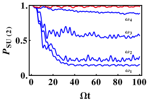
which attains its maximum value (of one) only when $\left|\psi\right\rangle$ is an atomic coherent state, and decreasing when it starts to deviate from it. From the phase space point of view, this deviation is greater when the state gets more delocalized over the Bloch sphere, for example, when the state of the system collapses in relative phase or number. Interestingly, the generalized purity can be related to the fringe visibility $\mathcal{V}$, of the interference pattern formed when the fragmented condensate is released from the trap and let to expand freely. The visibility is in fact given by $\mathcal{V}=\sqrt{\wp_{\,\,\textrm{SU(2)}}}$ (see the discussion concerning eq. (12) of [3] and compare with our eq. (13)). A high visibility is always desired in the context of BEC interferometry since it translates into a better resolution for phase measurements, and so is the generalized purity. Maximal visibility (of one) is attained for an atomic coherent state. However the same non-linearities due to interactions that make the condensate useful for quantum interferometry (due to squeezing) [7, 8], tend to diminish the visibility. This aspect is changed with the presence of a modulation in the scattering length. In fig. 5, the evolution of $\wp_{\,\,\textrm{SU(2)}}$ is plotted for different driving frequencies (blue) approaching from below the “resonance” value (red) used in fig. 4, with all the other parameters and initial state fixed. It is clear that exists a critical frequency which maintains the purity (and visibility) close to one which for the initial Fock-coherent state $\left|N\right\rangle$ is around the value 1.8$\Omega$. Though not shown in the figure, the purity also starts decreasing for higher frequencies.

Figure 5: Temporal evolution of the generalized purity $\wp_{\,\,\textrm{SU(2)}}$ (or squared visibility $\mathcal{V}^{2}$) for the same initial preparation as in fig. 4, with driving frequencies: $\omega_{1}=1.0$, $\omega_{2}=1.2$, $\omega_{3}=1.4$, $\omega_{4}=1.6$ (blue curves) below the critical value $\omega_{\textrm{c}}\thickapprox 1.8$ (red curve), indicating the approaching of the transition where the collapse of the semiclassical distribution is avoided.

Figure 6: (color online) Modulation parameters space diagram for the temporal average of the SU(2) purity measure (or squared visibility $\mathcal{V}^{2}$), taken during a time interval of $\Omega t=100$. The same initial state of fig. 4 was used. Note the weak dependence on the modulation amplitude $\mu$.

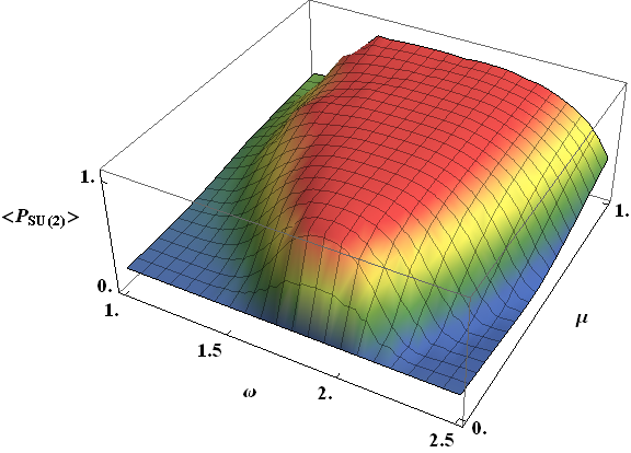
In order to analyze the robustness of this control and the influence of the amplitude of the modulation, it is plotted in Fig. 6 the temporal average of the purity as a function of the driving parameters $\omega$ and $\mu$, again for the same initial preparation; the time average was taken for an interval of 100 in units of $\Omega^{-1}$. It can be seen that effectively the maximum of the purity is reached for the critical frequency ($\omega=$1.8$\Omega$ in this particular case) and also the interesting feature that the control of coherence is not strongly dependent on the variation of the amplitude $\mu$, showing the same result for modulations going from 10 to 100% of the on-site static interaction $\kappa_{0}$. Other initial preparations, less conventional from an experimental point of view were considered, obtaining drastically different parameter diagrams indicating the chaoticity of our model owing to the non-linear interaction term in the Hamiltonian (7) and moreover its explicit time dependence. Those features are responsible for a high unpredictability of the stability regime of parameters. Nonetheless, the procedure of using the purity or equivalently the visibility has shown to be a valuable resource for finding regions of stability and can be employed in any practical scheme, since it is associated to standard procedures in BEC interferometry experiments.

5 Conclusions

In conclusion, by studying a scattering length modulated periodically in time it was found -for the case of a BEC in a double-well potential inside the Josephson regime- a possible way to control the phase and number diffusion of an initial coherent state. This avoidance of quantum collapse was visualized with the assistance of the $Q$-Husimi distribution, with the external driving field restraining the quantum distribution from spreading over the Bloch sphere phase space. This was further confirmed by the evolution of the generalized purity as a measure of the distance from a coherent state, which is directly related to the fringe visibility of the double-well interference. It was shown that this kind of control is strongly dependent on the driving frequency, with only a small influence from the amplitude of the modulation. This feature of a driven Bosonic Josephson junction can be of great interest for atom interferometry where various schemes for using this two-mode systems have been suggested and implemented. The reason is that by applying this technique, it is possible to turn off the undesired effects caused by the nonlinear interactions, allowing for longer holding times in the phase accumulation stage of the interferometer. We want to note that though the initial preparation shown in this paper is for the all-bosons-in-one-well Fock-coherent state, similar regions of stability can be found for other preparations as for example the typical balanced coherent state $\left|N/2\right\rangle$. Currently interactions are the principal limitation towards actual Heisenberg-limited metrology based on BECs. A future aspect to be considered is the extension of the present discussion for interferometry involving multiple traps, which has shown several promising features.

Appendix A Derivation of a Fokker-Planck equation for the Husimi $Q$-distribution on the Bloch sphere

We start from the von Neumann-Liouville equation

$$\frac{\partial\hat{\rho}}{\partial t}=-i[\hat{H},\hat{\rho}],$$ (14)

with $\hat{H}$ given in (1), and the goal is to obtain an equation for the time-evolution of the Husimi $Q$-distribution as a function of the angles $(\theta,\varphi)$ on the Bloch sphere. First we take the mean of equation (14) on a coherent state (9),

$$\frac{\partial Q}{\partial t} = -i\kappa\left\langle\theta,\varphi|[\hat{n}_{1}\left(\hat{n}_{1}-1\right)+\hat{n}_{2}\left(\hat{n}_{2}-1\right),\hat{\rho}]|\theta,\varphi\right\rangle$$ (15)

$$+i\frac{\Omega}{2}\left\langle\theta,\varphi|[\hat{a}_{1}^{\dagger}\hat{a}_{2}+\hat{a}_{1}\hat{a}_{2}^{\dagger},\hat{\rho}]|\theta,\varphi\right\rangle.$$

The first term of this equation, corresponding to the interaction, can be rewritten as

$$2i\kappa(N\left\langle\theta,\varphi|[\hat{n},\hat{\rho}]|\theta,\varphi\right\rangle-\left\langle\theta,\varphi|[\hat{n}^{2},\hat{\rho}]|\theta,\varphi\right\rangle)$$ (16)

with the definitions, $\hat{n}_{1}\equiv\hat{n}$ and $\hat{n}_{2}\equiv N-\hat{n}.$ Since in the Fock basis the density operator has the form $\hat{\rho}=\sum_{n,m=0}^{N}c_{n}c_{m}^{*}\left|n\right\rangle\left\langle m\right|,$ then the first commutator in (16) is evaluated as

$$[\hat{n},\hat{\rho}]=\sum_{n,m=0}^{N}c_{n}c_{m}^{*}(n-m)\left|n\right\rangle\left\langle m\right|,$$ (17)

and using the fact that

$$\left\langle\theta,\varphi\left|n\right\rangle\left\langle m\right|\theta,\varphi\right\rangle = \sqrt{{{N}\choose{n}}{{N}\choose{m}}}e^{i(n-m)\phi}\cos^{n+m}(\frac{\theta}{2})\;\sin^{2N-(n+m)}(\frac{\theta}{2}),$$ (18)

it is readily obtained the following identity:

$$\left\langle\theta,\varphi|[\hat{n},\hat{\rho}]|\theta,\varphi\right\rangle=-i\frac{\partial}{\partial\varphi}Q(\theta,\varphi;t).$$ (19)

A similar relation can be found for the anti-commutator,

$$\{\hat{n},\hat{\rho}\}=\sum_{n,m=0}^{N}c_{n}c_{m}^{*}(n+m)\left|n\right\rangle\left\langle m\right|,$$ (20)

taking the derivative of (18) with respect to $\theta$ and rearranging terms:

$$\left\langle\theta,\varphi|\{\hat{n},\hat{\rho}\}|\theta,\varphi\right\rangle = [N(1+\cos\theta)-\sin\theta\frac{\partial}{\partial\theta}]Q(\theta,\varphi;t)$$

Using eqs. (19) and (LABEL:eq:anti) in the second commutator in (16)

$$[\hat{n}^{2},\hat{\rho}]=\sum_{n,m=0}^{N}c_{n}c_{m}^{*}(n-m)(n+m)\left|n\right\rangle\left\langle m\right|,$$ (22)

it is obtained the identity

$$\left\langle\theta,\varphi|[\hat{n}^{2},\hat{\rho}]|\theta,\varphi\right\rangle=-i\frac{\partial}{\partial\varphi}[N(1+\cos\theta)-\sin\theta\frac{\partial}{\partial\theta}]Q(\theta,\varphi;t).$$ (23)

With these two identities the interaction term (16) can be written as

$$2\kappa(\sin\theta\frac{\partial^{2}}{\partial\theta\partial\varphi}-N\cos\theta\frac{\partial}{\partial\varphi})Q(\theta,\varphi;t).$$ (24)

For the tunneling term in (15) we proceed in an analogous manner, and after some algebra we obtain

$$-\Omega(\sin\varphi\frac{\partial}{\partial\theta}+\cot\theta\cos\varphi\frac{\partial}{\partial\varphi})Q(\theta,\varphi;t).$$ (25)

Note that this differential operator is exactly the orbital angular momentum operator around the $x$ axis. Collecting these two last results in the von Neumann-Liouville equation for $Q(\theta,\varphi;t)$, we finally obtain the Fokker-Planck equation

$$\frac{\partial Q(\theta,\varphi;t)}{\partial t} = [-\Omega(\sin\varphi\frac{\partial}{\partial\theta}+\cot\theta\cos\varphi\frac{\partial}{\partial\varphi})$$

$$-2\kappa(N\cos\theta\frac{\partial}{\partial\varphi}-\sin\theta\frac{\partial^{2}}{\partial\theta\partial\varphi})]Q(\theta,\varphi;t).$$

References

- [1] Bloch I, Hänsch T W and Esslinger T 2000 Nature 403 166
- [2] Andrews M R, Townsend C G, Miesner H J, Durfee D S, Kurn D M and Ketterle W 1997 Science 275 637
- [3] Gross C 2012 J. Phys. B 45 103001 and references therein
- [4] Sørensen A, Duan L M, Cirac J I and Zoller P 2001 Nature 409 63
- [5] Estève J, Gross C, Weller A, Giovanazzi S and Oberthaler M K 2008 Nature 4551216
-
[6]
Kitagawa M and Ueda M 1983 Phys. Rev. A 47 5138;
Wineland D J, Bollinger J J, Itano W M and Heinzen D J 1994 Phys. Rev A 50 67 - [7] Gross C, Zibold T, Nicklas E, Estève J and Oberthaler M K 2010 Nature 464 1165
- [8] Grond J, Hohenester U, Mazets I and Schmiedmayer J 2010 New J. Phys. 12 065036
[9]
Lewenstein M and You L 1996 Phys. Rev. Lett.
77 3489;
Wright E M, Walls D F and Garrison J C 1996 Phys. Rev. Lett. 77 2158;
Castin Y and Dalibard J 1997Phys. Rev. A 55 4430 - [10] Morsch O and Oberthaler M K 2006 Rev. Mod. Phys. 78 179
- [11] Chin C, Grimm R, Julienne P and Tiesinga E 2010 Rev. Mod. Phys. 82 1225
[12]
Khaykovich L, Schreck F, Ferrari G, Bourdel T, Cubizolles J, Carr L D, Castin Y, Salomon C 2002 Science
296 1290;
Strecker K E, Partridge G B, Truscott A G and Hulet R G 2002 Nature 417 150 -
[13]
Billy J, Josse V, Zuo Z, Bernard A, Hambrecht B, Lugan P, Clément D, Sanchez-Palencia L, Bouyer P and Aspect A 2008 Nature 453 891;
Roati G, D’Errico C, Fallani L, Fattori M, Fort C, Zaccanti M, Modugno G, Modugno M and Inguscio M 2008 Nature 453 895 - [14] Saito H and Ueda M 2003 Phys. Rev. Lett. 90 040403
- [15] Abdullaev F K, Kamchatnov A M, Konotop V V and Brazhnyi V A 2003 Phys. Rev. Lett. 90 230402
- [16] Kevrekidis P G, Theocharis G, Frantzeskakis D J and Malomed B A 2003 Phys. Rev. Lett. 90 230401
- [17] Liang Z X, Zhang Z D and Liu W M 2005 Phys. Rev. Lett. 94 050402
- [18] Abdullaev F K, Caputo J G, Kraenkel R A and Malomed B A 2003 Phys. Rev. A 67 013605
- [19] Staliunas K, Longhi S and de Valcárcel G J 2002 Phys. Rev. Lett. 89 210406
- [20] Nicolin A I, Carretero-González R and Kevrekidis P G 2007 Phys. Rev. A 76 063609
[21]
L. Henn E A, Seman J A, Roati G, Magalhães K M F
and Bagnato V S 2009 Phys. Rev. Lett. 103 045301;
Seman J A, Shiozaki R F, Poveda-Cuevas F J, Henn E A L, Magalhães K M F, Roati G and Bagnato V S 2011 J. Phys.: Conf. Ser. 264 012004 - [22] Albiez M, Gati R, Fölling J, Hunsmann S, Cristiani M and Oberthaler M K 2005 Phys. Rev. Lett. 95 010402
- [23] Greiner M, Mandel O, Hänsch T W and Bloch I 2002 Nature 419 51
- [24] Milburn G J, Corney J, Wright E M and Walls D F 1997 Phys. Rev. A 55 4318
- [25] Dalton B J and Ghanbari S 2011 J. Mod. Opt. 59 287
- [26] Moerdijk A J, Verhaar B J and Axelsson A 1997 Phys. Rev. A 51 4852
- [27] Inouye S, Andrews M R, Stenger J, Miesner H J, Stamper-Kurn D M and Ketterle W 1998 Nature 392 151
- [28] Pollack S E, Dries D, Hulet R G, Magalhães K M F, Henn E A L, Ramos E R F, Caracanhas M A and Bagnato V S 2010 Phys. Rev. A 81 053627
- [29] Schwinger J, Quantum Theory of Angular Momentum, edited by Biedenharn L C and van Dam H 1965 (Academic Press, New York) p. 229
- [30] Arecchi F T, Courtens E, Gilmore R and Thomas H 1972 Phys. Rev. A 6 2211
- [31] Pegg D T and Barnett S M 1989 Phys. Rev. A 39 1665
- [32] Raghavan S, Smerzi A, Fantoni S and Shenoy S R 1999 Phys. Rev. A 59 620
- [33] Wright E M, Walls D F and Garrison J C 1996 Phys. Rev. Lett. 77 2158
- [34] Holthaus M and Stenholm S 2001Eur. Phys. J. B 20 451
[35]
Barnum H, Knill E, Ortiz G and Viola L 2003 Phys.
Rev. A 68 032308;
Barnum H, Knill E, Ortiz G and Viola L 2004 Phys. Rev. Lett. 92 107902;
Somma R, Ortiz G, Barnum H, Knill E and Viola L 2004 Phys. Rev. A 70 042311 -
[36]
Klyachko A A, arXiv:quant-ph/020601v1;
Klyachko A A, Öztop B and Shumovsky A S 2007 Phys. Rev. A 75 032315 -
[37]
Viscondi T F, Furuya K and de Oliveira M C,
2009 Phys. Rev. A 80 013610;
Viscondi T F, Furuya K and de Oliveira M C 2010 Eur. Phys. Lett. 90 10014