Tunneling Current Spectra of a Metal Core/Semiconductor Shell Quantum Dot Molecule

Abstract

The transport properties of a metal core/semiconductor shell quantum dot molecule (QDM) embedded in a matrix connected to metallic electrodes are theoretically studied in the framework of Keldysh Green function technique. The effects of the electron plasmon interactions (EPIs) on the tunneling current spectra of QDM are examined. The energy levels of the QDs, intradot and interdot Coulomb interactions, electron interdot hopping strengths, and tunneling rates of QDs are renormalized by the EPIs. The differential conductance spectra show peaks arising from the plasmon assisted tunneling process, intradot and interdot Coulomb interactions, and coherent tunneling between the QDs.

I Introduction

Although many of the interesting transport phenomena related to quantum dots (QDs) including the Coulomb blockade,¹⁾ Kondo effect,²⁾ Fano resonance,³⁾ Pauli spin blockade,⁴⁾ photon (phonon) assisted tunneling process⁵⁾ and negative differential conductance,⁶⁾ have already been extensively studied, there has been little reported on the effects of electron plasmon interactions (EPIs) on the tunneling current of QDs. Recently, EPIs have received considerable attention for their applications in nanophotonics, biology, and the harvesting of solar energy.⁷⁾ Much effort has been focused on the effects of EPIs on the optical properties of nanostructures.^8-11) Experiments can observe the strong effect of EPIs on the exciton spectrum of individual semiconductor QDs arising from adjunctive metallic nanostructures^12,13).

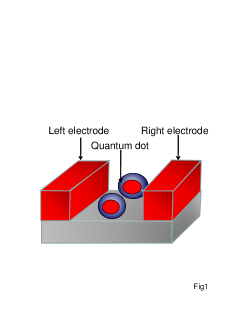
Figure 1: A metal core/semiconductor shell quantum dot molecule embedded in a matrix connected to metallic electrodes.

In the application of QD-based biosensor, the metal core/semiconductor shell QDs play an crucial role.¹⁴⁾ Because this type QDs can be readily coupled to detected proteins through electrostatic interactions. Despite the measurement of optical spectra can resolve molecules,^7-14) tunneling current spectra provide a high efficient means to identify molecules and address electrically a single nano-object.^15,16) This inspires us to study the tunneling current through individual metal core/semiconductor shell QDs for the application of nanoscale biosensor. However, it is difficult to avoid the proximity effect between such type QDs since QDs are randomly distributed.¹⁷⁾ Therefore, we consider a metal core/semiconductor shell QD molecule (QDM) embedded in a matrix connected to metallic electrodes shown in Fig. 1 to clarify how the EPIs to influence the proximity effect resulting from interdot electron Coulomb interactions, electron hopping process, and plasmon hopping between two QDs in the absence of detected proteins.

II Formalism

Here, we consider nanoscale semiconductor QDs, the energy levels separation of each QD is much larger than their on-site Coulomb interactions and thermal energies. One energy level for each quantum dot is considered in this study. The two-level Anderson model including EPIs is employed to simulate the QDM junction system as shown in Fig. 1. The Hamiltonian of the QDM junction is given by $H=H_{0}+H_{QDM}+H_{T}$

$$H_{0} = \sum_{k,\sigma}\epsilon_{k}a^{\dagger}_{k,\sigma}a_{k,\sigma}+\sum_{k,\sigma}\epsilon_{k}b^{\dagger}_{k,\sigma}b_{k,\sigma}$$

$$+ \sum_{k,\ell,\sigma}V_{k,\ell,L}d^{\dagger}_{\ell,\sigma}a_{k,\sigma}+\sum_{k,\ell,\sigma}V_{k,\ell,R}d^{\dagger}_{\ell,\sigma}b_{k,\sigma}+c.c$$

where the first two terms describe the free electron gas at the left and right metallic electrodes. $a^{\dagger}_{k,\sigma}$ ($b^{\dagger}_{k,\sigma}$) creates an electron of momentum $k$ and spin $\sigma$ with energy $\epsilon_{k}$ at the left (right) metallic electrode. $V_{k,\ell,\beta}$ ($\ell=1,2$) describes the coupling between the metallic electrodes and the QDs. $d^{\dagger}_{\ell,\sigma}$ ($d_{\ell,\sigma}$) creates (destroys) an electron in the $\ell$-th dot:

$$H_{QDM} = \sum_{\ell,\sigma}E_{\ell}n_{\ell,\sigma}+\sum_{\ell}U_{\ell}n_{\ell,\sigma}n_{\ell,\bar{\sigma}}$$

$$+ \frac{1}{2}\sum_{\ell,j,\sigma,\sigma^{\prime}}U_{\ell,j}n_{\ell,\sigma}n_{j,\sigma^{\prime}}+\sum_{\ell,j,\sigma}t_{\ell,j}d^{\dagger}_{\ell,\sigma}d_{j,\sigma},$$

where $E_{\ell}$ is the spin-independent QD energy level, and $n_{\ell,\sigma}=d^{\dagger}_{\ell,\sigma}d_{\ell,\sigma}$. Notations $U_{\ell}$ and $U_{\ell,j}$ describe the intradot and interdot Coulomb interactions, respectively. $t_{\ell,j}$ describes the electron interdot hopping. The Hamiltonian of QD molecule described by Eqs. (1) and (2) has already been extensively considered for studying the transport properties of nanostructures.^18-20) The Hamiltonian of electron plasmon interactions (EPIs) arising from the metallic nanostructure of each QDs can be written as $H_{T}$:

$$H_{T}=\sum_{\ell=1,2}\omega_{\ell}c^{\dagger}_{\ell}c_{\ell}+\sum_{\ell,\sigma}\Omega_{\ell}n_{\ell,\sigma}(c^{\dagger}_{\ell}+c_{\ell})-\sum_{i\neq\ell}\omega_{\ell,j}c^{\dagger}_{\ell}c_{j},$$ (3)

where $\omega_{\ell}$ is the plasmon frequency of the metallic nanostructures shown in Fig. 1, and $\Omega_{\ell}$ is the coupling strength of EPIs. The last term involving $\omega_{\ell,j}$ describes the plasmon hopping between two metallic nanostructures. When metal nanostructures are close enough, the plasmonic modes on one nanostructure can couple with that on other nanostructures so that hopping of plasmons from one metallic nanostructure to other nanostructure becomes possible.

A canonical transformation can be used to remove the on-site EPIs from Eq. (3), that is $H_{new}=e^{S^{\dagger}}He^{S}$, where $S=-\sum_{\ell,\sigma}\Omega_{\ell}n_{\ell,\sigma}(c^{\dagger}_{\ell}-c_{\ell})$.²¹⁾ In the new Hamiltonian, we have the following effective physical parameters: $V^{e}_{k,1.\alpha}=V_{k,1,\alpha}e^{\lambda_{1}(c^{\dagger}_{1}-c_{1})}$, $V^{e}_{k,2,\alpha}=V_{k,2,\alpha}e^{\lambda_{2}(c^{\dagger}_{2}-c_{2})}$, $E^{e}_{\ell}=E_{\ell}-\lambda^{2}_{\ell}\omega_{\ell}$, $U^{e}_{\ell}=U_{\ell}-2\lambda^{2}_{\ell}\omega_{\ell}$, $U^{e}_{\ell,j}=U_{\ell,j}-2\lambda_{1}\lambda_{2}\omega_{12}$, $t^{e}_{\ell,j}=t_{\ell,j}e^{-[\lambda_{1}(c^{\dagger}_{1}-c_{1})-\lambda_{2}(c^{\dagger}_{2}-c_{2})]}$, and $\lambda_{\ell}=\Omega_{\ell}/\omega_{\ell}$. In addition, $H_{new}$ has an extra term $\sum_{\ell\neq j,\sigma}\lambda_{\ell}\omega_{\ell,j}n_{\ell,\sigma}(c^{\dagger}_{j}+c_{j})$ resulting from the plasmon hopping between the metal nanostructures, which vanishes under free plasmon average introduced later. Under canonical transformation, we note that the narrowing of QD energy level broadening appears and QD energy levels, electron Coulomb interactions, and electron interdot hopping strengths become renormalized as well. The proximity effect between QDs resulting from $U^{e}_{\ell,j}$ and $t^{e}_{\ell,j}$ is influenced by the EPIs. It is possible to observe an effective negative interdot Coulomb interactions if we have strong EPIs and a large hopping matrix element of plasmon ($\omega_{\ell,j}$). For simplicity, this study is restricted in the case of $U^{e}_{\ell,j}\geq 0$ and identical QDs ($\omega_{\ell}=\omega_{0}$ and $\lambda_{\ell}=g$ ).

To decuple the EPIs of $H_{new}$, we take the mean-field average to remove the plasmon field arising from $c^{\dagger}-c$, that is $<e^{g(c^{\dagger}-c)}>=e^{-\frac{1}{2}g^{2}coth^{2}(\hbar\omega_{0}/(2k_{B}T))}$. Based on such a mean-field average, we see a reduction of $V_{k,\ell,\alpha}e^{-\frac{1}{2}g^{2}coth^{2}(\hbar\omega_{0}/(2k_{B}T))}=V_{k,\ell,\alpha}X_{\ell}$ and interdot hopping strength $t_{c}e^{-\frac{1}{2}(\lambda_{1}-\lambda_{2})^{2}coth^{2}(\hbar\omega_{0}/(2k_{B}T))}=t_{c}X_{\ell,j}=t_{c}$. This approximation is valid when the tunneling rate arising from the coupling between the QDs and the electrodes is smaller than the EPIs,²²⁾ which is our condition of interest. Based on such an approximation, the $\omega_{0}$-dependent tunelling rates are neglected in this study. Meanwhile, we assume that there is no voltage difference between two dots. This implies that the tunneling currents directly involving $t_{c}$ can be ignored.

Using the Keldysh-Green’s function technique,²³⁾ the tunneling currents of the QDMs in the Coulomb blockade regime are given by

$$J=\frac{-e}{h}\sum_{\ell,\sigma}\int d\epsilon\frac{\Gamma_{\ell,L}(\epsilon)\Gamma_{\ell,R}(\epsilon)}{\Gamma_{\ell,L}(\epsilon)+\Gamma_{\ell,R}(\epsilon)}ImG^{r}_{\ell,\sigma}(\epsilon)[f_{L}(\epsilon)-f_{R}(\epsilon)]$$ (4)

where $f_{L(R)}(\epsilon)=1/[e^{(\epsilon-\mu_{L(R)})/k_{B}T}+1]$ denotes the Fermi distribution function of the left (right) electrode. The left (right) chemical potential is given by $\mu_{L}(\mu_{R})$. $\mu_{L}-\mu_{R}=eV_{a}$, where $V_{a}$ denotes the applied bias. Notation $T$ denotes the equilibrium temperature of the left and right electrodes. $e$ and $h$ denote the electron charge and Planck’s constant, respectively. Notation $\Gamma_{\ell,L(R)}=\sum_{k}V^{2}_{k,\ell,L(R)}\delta(\epsilon-\epsilon_{k})$ denotes the tunnelling rate from the left (right) electrode to dot 1 and dot 2, which is assumed to be energy- and bias-independent. The retarded Green function of the QD density of states ($-ImG^{r}_{\ell,\sigma}$) has the following expression

$$G^{r}_{\ell,\sigma}(\epsilon) = \sum^{\infty}_{n=-\infty}L_{n}[f^{<}(\epsilon+n\omega_{0}){\cal G}^{r}_{\ell,\sigma}(\epsilon+n\omega_{0})$$

$$+ f^{>}(\epsilon-n\omega_{0}){\cal G}^{r}_{\ell,\sigma}(\epsilon-n\omega_{0})],$$

where $L_{n}$ is given by

$$L_{n}(\epsilon)=e^{-g^{2}(1+N_{B})}e^{\frac{n\omega_{0}}{2k_{B}T}}I_{n}(2g^{2}\sqrt{N_{B}(1+N_{B})})$$ (6)

with a boson distribution function of $N_{B}=1/(e^{\hbar\omega_{0}/(k_{B}T)}-1)$, and a Bessel function of $I_{n}(x)$. The expressions of $f^{<}(\epsilon+n\omega_{0})$ and $f^{>}(\epsilon-n\omega_{0})$ are

$$f^{<}(\epsilon+n\omega_{0})=\frac{\Gamma^{e}_{\ell,L}f_{L}(\epsilon+n\omega_{0})+\Gamma^{e}_{\ell,R}f_{R}(\epsilon+n\omega_{0})}{\Gamma^{e}_{\ell,L}+\Gamma^{e}_{\ell,R}},$$ (7)

and

$$f^{>}(\epsilon-n\omega_{0})=1-\frac{\Gamma^{e}_{\ell,L}f_{L}(\epsilon-n\omega_{0})+\Gamma^{e}_{\ell,R}f_{R}(\epsilon-n\omega_{0})}{\Gamma^{e}_{\ell,L}+\Gamma^{e}_{\ell,R}},$$ (8)

where the effective tunneling rate of $\Gamma^{e}_{\ell,L(R)}=\Gamma_{\ell,L(R)}X^{2}$ with the reduction factor of $X=exp[-\frac{1}{2}g^{2}coth^{2}(\hbar\omega_{0}/(2k_{B}T))]$. The dressed electron retarded Green function under $H_{new}$ can be obtained following the procedure introduced in our previous work.²⁰⁾ We have the expression of ${\cal G}^{r}_{\ell,\sigma}$

$${\cal G}^{r}_{\ell,\sigma}(\epsilon)=\sum^{8}_{m=1}{\cal G}^{r}_{\ell,m,\sigma}(\epsilon)=\sum_{m=1}^{8}\frac{p_{m}}{\mu_{\ell}-\Sigma_{m}},$$ (9)

where $\mu_{\ell}=\epsilon-E^{e}_{\ell}+i\Gamma^{e}_{\ell}/2$. $\Gamma^{e}_{\ell}=(\Gamma_{\ell,L}+\Gamma_{\ell,R})X^{2}$. The sum of $m$ in Eq. (9) has over 8 possible configurations. We consider an electron (of spin $\sigma$) entering level $\ell$, which can be either occupied (with probability $N_{\ell,\bar{\sigma}}$) or empty (with probability $1-N_{\ell,\bar{\sigma}}$). For each case, the level $j$ can be empty (with probability $a_{j}=1-N_{j,\sigma}-N_{j,\bar{\sigma}}+c_{j}$), singly occupied in a spin $\bar{\sigma}$ state (with probability $b_{j,\bar{\sigma}}=N_{j,\bar{\sigma}}-c_{j}$) or spin $\sigma$ state (with probability $b_{j,\sigma}=N_{j,\sigma}-c_{j}$), or a double-occupied state (with probability $c_{j}$). Thus, the probability factors associated with the 8 configurations appearing in Eq. (9) become $p_{1}=(1-N_{\ell,\bar{\sigma}})a_{j}$, $p_{2}=(1-N_{\ell,\bar{\sigma}})b_{j,\bar{\sigma}}$, $p_{3}=(1-N_{\ell,\bar{\sigma}})b_{j,\sigma}$, $p_{4}=(1-N_{\ell,\bar{\sigma}})c_{j}$, $p_{5}=N_{\ell,\bar{\sigma}}a_{j}$, $p_{6}=N_{\ell,\bar{\sigma}}b_{j,\bar{\sigma}}$, $p_{7}=N_{\ell,\bar{\sigma}}b_{j,\sigma}$, and $p_{8}=N_{\ell,\bar{\sigma}}c_{j}$. $\Sigma_{m}$ in the denominator of Eq. (9) denotes the self-energy correction due to Coulomb interactions and coupling with level $j$ in configuration $m$. We have $\Sigma_{1}=t_{c}^{2}/\mu_{j}$, $\Sigma_{2}=U^{e}_{\ell,j}+t_{c}^{2}/(\mu_{j}-U^{e}_{j})$, $\Sigma_{3}=U^{e}_{\ell,j}+t_{c}^{2}/(\mu_{j}-U^{e}_{j,\ell})$, $\Sigma_{4}=2U^{e}_{\ell,j}+t_{c}^{2}/(\mu_{j}-U^{e}_{j}-U^{e}_{j,\ell})$, $\Sigma_{5}=U^{e}_{\ell}+t_{c}^{2}/(\mu_{j}-U^{e}_{j,\ell})$, $\Sigma_{6}=U^{e}_{\ell}+U^{e}_{\ell,j}+t_{c}^{2}/(\mu_{j}-U^{e}_{j}-U^{e}_{j,\ell})$, $\Sigma_{7}=U^{e}_{\ell}+U^{e}_{\ell,j}+t_{c}^{2}/(\mu_{j}-2U^{e}_{j,\ell})$, and $\Sigma_{8}=U^{e}_{\ell}+2U^{e}_{\ell,j}+t_{c}^{2}/(\mu_{j}-U^{e}_{j}-2U^{e}_{j,\ell})$. Note that the fractional numbers of the thermally averaged one-particle occupation number $N_{\ell,\sigma}$ and two-particle correlation functions $c_{\ell}$ appear only on the probability weights of ${\cal G}^{r}_{\ell,m,\sigma}$. Once $t_{c}=0$ and $g=0$, the expression of Eq. (9) is the same as Eq. (3) in Ref. 6. $N_{\ell,\sigma}$ and $c_{\ell}$ can be obtained by solving the on-site lesser Green’s functions,²⁰⁾ their expressions are

$$N_{\ell,\sigma}=-\int\frac{d\epsilon}{\pi}\sum^{8}_{m=1}\frac{\Gamma^{e}_{\ell}f_{\ell}(\epsilon)+\Gamma^{e}_{j}f_{j}(\epsilon)}{\Gamma^{e}_{\ell}+\Gamma^{e}_{j}}Im{\cal G}^{r}_{\ell,m,\sigma}(\epsilon),$$ (10)

and

$$c_{\ell}=-\int\frac{d\epsilon}{\pi}\sum^{8}_{m=5}\frac{\Gamma^{e}_{\ell}f_{\ell}(\epsilon)+\Gamma^{e}_{j}f_{j}(\epsilon)}{\Gamma^{e}_{\ell}+\Gamma^{e}_{j}}Im{\cal G}^{r}_{\ell,m,\sigma}(\epsilon).$$ (11)

Note that $\ell\neq j$ in Eqs. (9)-(11), which are valid in the condition of $t_{c}/U_{\ell}\ll 1$. In addition, the limitation of $0\leq N_{\ell,\sigma}(c_{\ell})\leq 1$ should be satisfied.

III Results and Discussion

Bulk metals have very large plasmon frequencies, which can be ten times larger than the on-site Coulomb interactions of QDs. Therefore, the effects of EPIs on the tunneling current were ignored in the previous studies.^18-20) The plasmon frequency of metallic nanostructures is the same order of magnitude as the on-site Coulomb interactions and the EPIs is strong.¹³⁾ One can expect to observe the plasmon assisted tunneling processes in the tunneling current spectra. To reveal the effects of EPIs on the tunneling current spectra of QDMs, we initially consider the case without EPIs. The tunneling current and differential conductance are plotted in Fig. 2 with $U_{\ell}=U_{0}=60\Gamma_{0}$, $U_{\ell,j}=U_{I}=20\Gamma_{0}$, and $E_{\ell}=E_{0}+\eta_{\ell}eV_{a}$. There is a large voltage across the junction, therefore the shift of energy level $E_{\ell}$ arising from the applied bias is considered by $\eta_{\ell}eV_{a}$. We have adopted $\eta_{\ell}=0.5$ based on the assumption that QDs are located in the central position between two electrodes. The black lines show the typical staircase structure of the tunneling current and an oscillatory differential conductance with respect to the applied bias arising from the intradot Coulomb interactions. These structures will be washed out with increasing temperature. We will focus on the transport behavior throughout at the low temperature of $k_{B}T=1\Gamma_{0}$. In the presence of interdot Coulomb interactions (red lines), new staircase structures appear in the tunneling current. Five peaks in differential conductance labeled from $V_{1}$ to $V_{5}$ result from electrons of the left electrode through the resonant channels of $\epsilon_{1}=E_{0}$, $\epsilon_{2}=E_{0}+U_{I}$, $\epsilon_{3}=E_{0}+U_{0}$, $\epsilon_{4}=E_{0}+U_{0}+U_{I}$, and $\epsilon_{5}=E_{0}+U_{0}+2U_{I}$. In the presence of $t_{c}$ (see the blue lines), each peaks ($V_{1},V_{2},V_{4}$ and $V_{5}$) split into the bonding (BD) and antiboding (ABD) states. Such structures can be depicted by using a single molecule with $E_{0}-t_{c}$ and $E_{0}+t_{c}$ states filled with one, two, three and four electrons. The electron filling of such a QDM satisfies Hund’s rule. In addition, peaks $V_{2}$ and $V_{4}$ have extra peaks, which correspond to the spin singlet states (two electrons and three electrons). For instance the two electron singlet state has a resonant pole $\epsilon=E_{0}+U_{I}-t^{2}_{c}/(U_{0}-U_{I})$ resulting from the $p_{2}$ in Eq. (9), which is different from the two electron triplet state with pole $\epsilon=E_{0}+U_{I}\pm t_{c}$ from the $p_{3}$ of Eq. (9). The differential conductance structure resulting from three electrons can also be analyzed from the $p_{6}$ and $p_{7}$ of Eq. (9). On the basis of results in Fig. 2, we find that the interdot Coulomb interactions play an important role in distinguishing between the configurations of one electron, two electrons, three electrons and four electrons. Many theoretical works have been devoted to investigate the tunneling current through parallel QDs for the applications of quantum computing.²⁴⁾ Nevertheless, there still lacks a comprehensive theory to reveal the spin states of parallel QDs. The retarded Green function of Eq. (9) provides a closed form expression to distinguish eight configurations in the parallel QDs.

Figure 3 shows the tunneling current (J) and differential conductance (dG) for different strengths of EPIs at $U_{0}=60\Gamma_{0}$, $U_{I}=20\Gamma_{0}$, $t_{c}=0$, $\omega_{i,j}=\omega_{0}=20\Gamma_{0}$. With increasing the strength of EPIs, the energy levels of the QDs, intradot Coulomb interactions, and interdot Coulomb interactions are renormalized by EPIs such as $E^{e}_{\ell}=E_{\ell}-g^{2}\omega_{0}$, $U^{e}_{\ell}=U_{\ell}-2g^{2}\omega_{0}$, and $U^{e}_{\ell,j}=U_{\ell,j}-2g^{2}\omega_{0}$. The current spectra and differential conductance change considerably. Five peaks of dG labeled from $V_{1}$ to $V_{5}$ at g=0 are shifted to the low bias regime. The magnitude and width of these peaks become smaller and narrower with increasing $g$. This is attributed to the current reduction factor of $e^{-g^{2}(1+N_{B})}$ [see Eq. (6)] and reduction of the tunneling rates $\Gamma^{e}_{\ell}=\Gamma_{\ell}X^{2}$. In addition to these five peaks, there is a satellite peak labeled n=1, which arises from one plasmon assisted tunneling process. For the blue line, we see two one-plasmon assisted tunneling peaks corresponding to $\epsilon=E^{e}_{0}+\omega_{0}$, and $\epsilon=E^{e}_{0}+U^{e}_{I}+\omega_{0}$. As a consequence of the very low temperatures, the structures arising from $\epsilon=E^{e}_{0}-\omega_{0}$, and $\epsilon=E^{e}_{0}+U^{e}_{I}-\omega_{0}$, which are contributed from the first term of Eq. (5), correspond to electrons of the QDM with energy levels $E^{e}_{0}$ and $E^{e}_{0}+U^{e}_{I}$ to have one plasmon emission process to escape out the QDM. This processes are obviously suppressed in the small bias regime resulting from small electron population of the QDM.

Since we consider $t_{c}=0$, the spin degree of freedom can not be resolved in Fig. 3.⁶⁾ To further understand the EPIs on the current spectra of QDMs with finite $t_{c}$, we plot the tunneling current (J) and differential conductance (dG) as a function of the applied bias for the case of $U_{\ell}=100\Gamma_{0}$, $U_{\ell,j}=40\Gamma_{0}$, and $t_{c}=6\Gamma_{0}$ in Fig. 4. The first two peaks indicated by the black line for dG correspond to the BD and ABD states. The following three peaks are similar to those indicated by the blue line in Fig.2. They result from the spin singlet and triplet states. For $g=0.5$, these spin-dependent spectra of dG just shift to the low bias regimes, whereas the separation between the BD and ABD peaks in the triplet state is not changed. The exchange energy of the singlet state $-t^{2}_{c}/(U^{e}_{\ell}-U^{e}_{\ell,j})$ is also invariant. For $g=1$, the tunneling currents are enhanced resulting from the absence of the interdot Coulomb blockade. The spectra from the two particle states merge into that of one particle at $g=1$. Consequently, the spin-dependent spectra of dG is suppressed. In addition, we observe multiple plasmon assisted tunneling processes (n=2).

IV Summary and conclusions

In this study we analyzed the effects of homogenous EPIs on the tunneling current spectra of QDMs in the absence of detected proteins. As a result of the renormalization of the energy levels of QDs, intradot and interdot Coulomb interactions, and the tunneling rates, there is a significant change in the tunneling current spectra for strong EPIs coupling. Because of the hopping of plasmons between two metal nanostructures, the indirect interdot plasmon mediated electron electron Coulomb interactions appear. We predict that the multiple plasmon assisted tunneling processes can be observed in the tunneling current spectra of metal core/shell semiconductor QDs for strong EPIs. In the presence of detected proteins, which will glue to the QDMs, the DOS of QDMs is changed. Therefore, the measured tunneling current spectra are tilted to judge the identity of detected proteins.

Acknowledgments This work was supported by the National Science Council of Taiwan under Contract No: NSC 101-2112-M- 008-014-MY2.

E-mail: mtkuo@ee.ncu.edu.tw

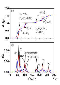
Figure 2: (a) Tunneling current J and (b) differential conductance $dG=dJ/dV_{a}$ as a function of the applied bias for $U_{\ell}=U_{0}=60\Gamma_{0}$, $E_{\ell}=E_{F}+30\Gamma_{0}$, $k_{B}T=1\Gamma_{0}$, and $\Gamma_{\ell,L}=\Gamma_{\ell,R}=0.5\Gamma_{0}$ in the absence of electron plasmon interactions. Black lines ($U_{\ell,j}=0$), red lines ($U_{\ell,j}=20\Gamma_{0}$ and $t_{c}=0$), and blue lines ($U_{\ell,j}=20\Gamma_{0}$ and $t_{c}=6\Gamma_{0}$). Note that the tunneling current J is in units of $J_{0}=e\Gamma_{0}/h$.

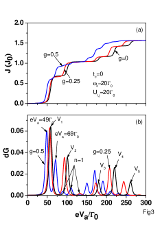
Figure 3: (a) Tunneling current J and (b) differential conductance $dG$ as a function of the applied bias in the presence of electron plasmon interactions. Black lines ($g=0.0$), red lines ($g=0.25$), and blue lines ($g=0.5$). We have a plasmon frequency $\omega_{0}=20\Gamma_{0}$. The other physical parameters are the same as those for the red lines in Fig.2.

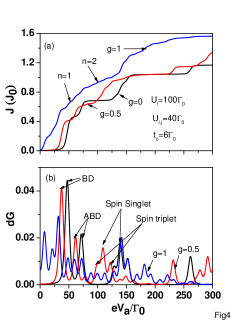
Figure 4: (a) Tunneling current J, and (b) differential conductance $dG$ as a function of the applied bias for different g values. Black lines ($g=0$), red lines ($g=0.5$), and blue lines ($g=1$). We have adopted the following physical parameters:$U_{\ell}=100\Gamma_{0}$, $U_{\ell,j}=40\Gamma_{0}$, $t_{c}=6\Gamma_{0}$, $k_{B}T=1\Gamma_{0}$, and $\Gamma_{\ell,L}=\Gamma_{\ell,R}=0.5\Gamma_{0}$.

References

• (1) C. Livermore,C. H. Crouch,R. M. Westervelt, , K. L. Campman, and A. C. Gossard: Science 274, (1996) 1332.
• (2) S. M. Cronenwett,T. H. Oosterkamp, and L. P. Kouwenhoven: Science 281 (1998) 540.
• (3) A. A. Clerk, X. Waintal, and P. W. Brouwer: Phys. Rev. Lett. 86, (2001) 4636.
• (4) K. Ono, D. G. Austing, Y. Tokura, and S. Tarucha: Science 297, (2002) 1313.
• (5) C. A. Stafford and N. S. Wingreen: Phys. Rev. Lett. 76, (1996) 1916.
• (6) David. M. T. Kuo, and Y. C. Chang: Phys. Rev. Lett. 99, (2007) 086803.
• (7) J. A. Scholl, A. L. Koh, and J. A. Dionne: Nature 483, (2012) 421.
• (8) D. J. Bergman, and M. I. Stockman: Phys. Rev. Lett. 90, (2003) 027402.
• (9) J. Z. Li, and C. Z. Ning: Phys. Rev. Lett. 93, (2004) 087402.
• (10) G. Schull, N. Neel, P. Johansson, and R. Berndt: Phys. Rev. Lett. 102, (2009) 057401.
• (11) J. T. Zhang, Y. Tang,K. Lee, and M. Ouyang: Nature 466, (2010) 91.
• (12) C. H. Eyal, W. B. Garnett, P. Iddo, S. Joseph, and B . J. Israel: Nano Lett. 12, (2012) 4260.
• (13) T. K. Halkala, J. J. Toppari, A. Kuzyk, M. Pettersson, H. Tikkanen, H. Kuntuu, and P. Torma: Phys. Rev. Lett. 103, (2009) 053602.
• (14) X. J. Ji, J. Y. Zheng, J.M. Xu, V. K. Rastogi, T. C. Cheng, J. J. DeFrank, and R. M. Leblanc: J. Phys. Chem B 109, (2005) 3793.
• (15) A. P. Ivanov, E. Instuli, C. M. McGilvery, G. Baldwin, D. W. McComb, T. Albrecht, and J. B. Edel: Nano Lett. 11, (2011) 279.
• (16) Y. D. Guo, X. H. Yan, Y. Xiao: J. Phys. Chem C 116, (2012) 21609.
• (17) C. J. Zhong and M. M. Maye: Adv. Mater. 13, (2001) 1507.
• (18) W. G. van der Wiel, S. D. De Franceschi, J. M. Elzerman, T. Fujisawa, S. Tarucha, and L. P. Kouwenhoven: Rev. Mod. Phys. 75, (2003) 1.
• (19) Y. C. Chang and D. M. T. Kuo: Phys. Rev. B 77, (2008) 245412.
• (20) David. M. T. Kuo, S. Y. Shiau, and Y. C. Chang: Phys. Rev. B 84, (2011) 245303.
• (21) G. D. Mahan, Many-Particle Physics, (Kluwer Academic, New York 2000).
• (22) Z. Z. Chen, R. Lu, and B. F. Zhu: Phys. Rev. B 71, (2005) 165324.
• (23) A. P. Jauho, N. S. Wingreen, and Y. Meir: Phys. Rev. B 50, (1994) 5528.
• (24) D. S. Saraga and D. Loss: Phys. Rev. Lett. 90, (2003) 166803.
Refer to caption