Link Prediction with Social Vector Clocks

Abstract

State-of-the-art link prediction utilizes combinations of complex features derived from network panel data. We here show that computationally less expensive features can achieve the same performance in the common scenario in which the data is available as a sequence of interactions. Our features are based on social vector clocks, an adaptation of the vector-clock concept introduced in distributed computing to social interaction networks. In fact, our experiments suggest that by taking into account the order and spacing of interactions, social vector clocks exploit different aspects of link formation so that their combination with previous approaches yields the most accurate predictor to date.

social networks, vector clocks, link prediction, online algorithms

1 Introduction

Link prediction deals with predicting previously unobserved interactions among actors in a network [1]. Predictions are based on the dynamic network of previously observed interactions, which is usually made available in one of two forms: panel data or event data. The former refers to a sequence of complete network snapshots and typically contains only coarse-grained temporal information. Event data, on the other hand, consists of a finer-grained sequence of single, time-stamped relational events, in which the exact minute or second of each event is known. Whereas panel data is often collected by means of longitudinal surveys, event data is typically the outcome of automated data collection, such as log files of e-mail, phone, or Twitter communication.

It is possible to convert network event data into (interval-censored) network panel data; indeed, Liben-Nowell and Kleinberg [2] did so in their seminal paper which introduced the link prediction problem for social networks, and the practice has become standard [1, 3]. The conversion is usually carried out by defining a sequence of time slices and aggregating relational events within these time windows into static (weighted) networks. At the expense of losing the ordering and spacing of original events, this conversion allows one to employ the large set of tools that have been developed for static and longitudinal network analysis [4, 5].

Whether the conversion from event to panel data is justifiable or not depends crucially on mechanisms which drive tie formation in a given network. For example, Liben-Nowell and Kleinberg [2] conducted experiments on future interactions in large co-authorship networks. In this setting, the exact sequence and spacing of publication dates can hardly be relevant because publications dates are distorted anyway (backlogs, preprints, etc.); aggregation of publication events on a coarser time-scale thus does not appear to be problematic.

In other situations the fine-grained temporal information may be highly relevant, making the conversion from event data to panel data difficult to justify because it may destroy important patterns of interaction; see [6] for a recent review on general temporal network approaches to exploit such information. With regard to the link prediction problem, if we are trying to foresee whether node A will send an email message to B in the near future, for example, then an extremely useful piece of information is whether B has recently sent A a message; if so, it is likely that A will respond to B soon. This response-mechanism is known as reciprocity, and has been observed to be highly relevant for predicting future events in social networks [7]. By aggregating communication events into cross-sectional graphs, traditional link prediction schemes are generally prone to miss such simple and useful mechanisms.

Here, we demonstrate that link predictors can indeed be made more effective and efficient if they operate directly on appropriate time-stamped dyadic communication data, and as a result can take advantage of the information contained in the spacing and ordering of relational events. The approach we introduce is based on keeping track of how out of date a node A is with respect to another node B with respect to time-respecting information flow, and for doing so we employ the concept of vector clocks. Our results confirm that dyadic features that exploit fine-grained temporal information can be highly relevant for predicting which actors will communicate for the first time in the near future, and are not limited to reciprocity.

The outline is as follows: first, we describe the types of data for which we expect fine-grained temporal data to be relevant for link prediction. Next, we review the link prediction problem for this type of data, paying particular attention to supervised link prediction, a framework that we employ here. We then specify how a modified version of social vector clocks can be used as a supervised link predictor, and proceed to evaluate this predictor. We conclude with a discussion of our results, as well as possible future work.

2 Motivation

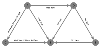
Figure 1: Illustrative example of social network data containing fine-grained information on dyadic communication events. Indirect information might flow on time-respecting paths, i.e. along labels that respect the ordering of time. Adapted from [16].

In the introduction, we stressed that the ordering and spacing of communication events might contain valuable additional information over and above the mere number of contacts between a pair of actors. Consider the example in Figure 1, which depicts a series of directed communication events, such as e-mail messages. Let us imagine that the actor represented by node A is in charge of organizing a wellness weekend-trip for a group of friends, and that she keeps changing her mind about when and where to go. She finally settles on a plan on Thursday at noon, and all of the subsequent messages she sends out include the final trip details. We can ask: which nodes can possibly know them, given the observed interactions? Clearly, node A communicated with node C after she made up her mind on Thursday, so node C would have received the final information on Friday at 9am. Because node C subsequently sent node B a message, node B could also have received the correct information. On the other hand, nodes D and E could not have received information from node A that is more recent than Wednesday at 3pm.

Two key and related concepts present in this example are latency and indirect updates. We expect that groups of people who coordinate some action, such as a wellness weekend-trip, will need to synchronize their knowledge of certain key information such as departure time and destination. So in some sense (which we will define formally in Section 4) the members of this group have a low latency with respect to each other. Indirect updates, such as the one that made B aware of A’s latest trip plans, are an important mechanism for maintaining these low latencies: even though B did not have any direct message from A after she made up her mind, B still got the latest plans indirectly via C.

This type of indirect communication is common in social systems: consider the case of several adult siblings who communicate with each other rarely, and more often communicate with their parents. In this case, the siblings’ information on each other can remain up to date due to the central role of the parents, who provide the siblings with an indirect means of communication. More generally, we observe that gossip – the information exchanged when two people talk about an absent third party – is a form of communication prevalent in society and is in essence a form of indirect update.

The motivation behind our approach in this paper is that this diffusion of information via indirect updates is common in many social systems, and can be exploited to infer future direct relations. In terms of the example above, we might predict that the siblings are likely to communicate with each other because their latencies with respect to each other remain low. However, the current approach to link prediction throws away much of these temporal clues by first converting the event stream into panel data.

In the datasets we analyze here, we also have reason to believe that fine-grained diffusion patterns are relevant to link prediction. For instance, two of the datasets that we will use during our evaluation contain sequences of micro-blogging events that come from Twitter. Bakshy et al. [8], e.g., have found that word-of-mouth information in Twitter spreads via many small cascades of tweets, mostly triggered by ordinary individuals. These small chains of diffusion are exemplary of the indirect updates we described above, and by considering the details of how information spread, we may be able to infer which nodes will come into direct contact in the future. Detailed information on the datasets we use in our final evaluation is given in Section 5.1.

3 Link Prediction

In this section, we review the basics of link prediction. In particular, we provide an overview of how machine learning models can be used to combine multiple link predictors – a technique called supervised link prediction.

3.1 The Problem and its Evaluation

Along the lines of its original formulation by Liben-Nowell and Kleinberg [2], we formulate the link prediction problem for dyadic event data as follows:

Given a sequence of communication events in the form of (time, sender, receiver) tuples, predict which pairs of nodes who had no communication (i.e. are disconnected) in the time interval $[t_{0},t_{1})$ will communicate (i.e. become connected) in the time interval $[t_{1},t_{2})$.

An unsupervised link predictor is a function which, given a dyad (a pair of nodes) and the list of all previously occurring events, returns a score, where a higher score indicates that an edge is more likely to form in the dyad. Common neighbors is an example of an unsupervised link predictor: given a dyad (A,B), return the number of contacts shared by A and B. Although common neighbors is simple, it is quite effective and many of the most effective unsupervised link predictors (such as the similarity measure originally proposed by Adamic and Adar [9]) are also based on shared neighbors [2, 3].

By running a link predictor on all dyads that are disconnected in the interval $[t_{0},t_{1})$, one can rank all of the possible new links. To evaluate a link predictor, we compare this ranking with the set of new dyads that actually occur in the period $[t_{1},t_{2})$. In practice, performance on the link-prediction task is often measured using ROC curves or measures based on precision, but in their recent paper on evaluation in the link prediction problem, Lichtenwalter and Chawla [1] convincingly argue that due to the extreme class imbalance present in the link prediction task, precision-recall curves are a more relevant and less deceptive way to measure performance. For that reason, here we exclusively use precision-recall curves for our evaluation.

3.2 Supervised link prediction

As link prediction is fundamentally a binary classification problem, it is natural to use the powerful binary classification models that have been developed in machine learning. The primary advantage of this approach is the ability to combine multiple unsupervised link predictors into one joint prediction model. We will now provide a brief overview of how supervised link prediction works. For an in-depth discussion of supervised link prediction, see [10].

As is usual in machine learning evaluation, we train and test our classifier on two separate datasets: we must be careful that the classifier is not trained on the same data that is used to evaluate it. For this reason, supervised link prediction requires a train and test framework as depicted in the bottom half of Figure 2. A link prediction classifier is given a set of features related to each disconnected dyad in the period $[t_{0},t_{1})$, as well as a label which indicates whether the dyad became connected in the period $[t_{1},t_{2})$. From this information, it learns a model which relates the dyad features to the probability that a previously disconnected dyad becomes connected. To measure the accuracy of a link predictor, we then create a set of test dyad features in the interval $[t^{\prime}_{0},t^{\prime}_{1})$ and use those to score the test labels in the interval $[t^{\prime}_{1},t^{\prime}_{2})$. We measure how accurately the scored dyads predict the set of test labels using the area under the precision-recall curve (AUPR).

We note that the AUPR of a link predictor can fluctuate greatly: as the behavior of users changes, so does the accuracy of the link predictor. In order to better estimate the typical AUPR attained by a link predictor, we can run this procedure many times; we will refer to each run of the procedure outlined in the bottom panel of Figure 2 as a realization. As shown in the top panel of Figure 2, we shift realizations such that the AUPR of each realization is measured using a distinct set of events.

Figure 2: Framework for performing and evaluating supervised link prediction. Each dataset is split into several realizations; each realization, in turn, is split into intervals to train and test a classifier.

Lichtenwalter et al. [10] convincingly argue that the link prediction problem should be stratified over different geodesic distances (i.e., path lengths). That is, the disconnected dyads with a geodesic distance of $N=2,3,4,\ldots$ should each be put into different bins, and a separate classifier should be trained on each bin. This stratification leads to better performance because the decision boundary for each bin can be quite different, with local features (such as common neighbors) being of primary importance at small distances, and global features (such as preferential attachment) becoming more important at larger distances. Thus, by treating each distance as a separate classification task, not only does performance improve, but one can also gain insight into the particular strengths and weaknesses of a predictor. We therefore follow suit and treat each distance as a separate link prediction task.

4 Learning with Vector Clocks

Having introduced the necessary background on network event data and link prediction, we now explain how fine-grained temporal information can be exploited, using the concept of vector clocks.

4.1 Traditional Vector Clocks

Vector clocks were conceptually defined in [11] and [12] as a means to track causality in concurrent systems, but had implicitly been used before, e.g., in [13], with underlying foundations attributed to [14]; for an introduction to vector clock systems in distributed computing refer to [15]. Kossinets et al. [16] brought the concept to social network analysis by substituting message-exchanging processes with communicating individuals. In this special setting, the basic motivation of vector clocks is to keep track of the lower bound of how out-of-date a person is with respect to every other person at any time, assuming that information spreads according to a given time-ordered list of communication events.

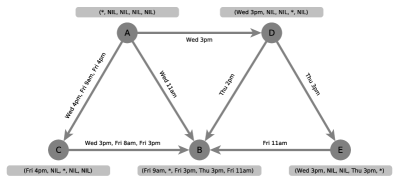
Figure 3: The basic idea of vector clocks: each node’s vector clock (in grey) keeps track of the most recent information it could have on the other actors in the network.

Reconsider the trip-planning example we introduced in Section 2. There we asked: which nodes could possibly know about the most recent details, through either direct or indirect updates? Vector clocks provide a way of answering this question by keeping track of the last possible update that a node could have received from each other node: the vector clock (grey box) next to node E in Figure 3 indicates that E cannot possibly have received information from A more recent than Wednesday at 3pm, that it could have received no information whatsoever from nodes B and C, and so on. Each node is always assumed to have up-to date information on itself.

Formally, let $(t_{i},s_{i},r_{i})$, $i\in\mathbb{N}$, a sequence of (time,sender,receiver) tuples satisfying $t_{i}\leq t_{i+1}$ and $s_{i}\not=r_{i}$. The set of individuals is defined implicitly by $V=\bigcup_{i\in\mathbb{N}}\{s_{i},r_{i}\}$. At time $t_{i}$, sender $s_{i}$ and receiver $r_{i}$ exchange direct information about themselves, and indirect information about others that result from communication events in the past ($t<t_{i}$). That is, information can not be forwarded instantaneously but with arbitrary small delay. Now, a vector clock is a multivariate function $\phi_{v,t}=(\phi_{v,t}(u):u\in V)$, in which $v$’s temporal view $\phi_{v,t}(u)$ on $u$ at time $t$ is defined as the time-stamp $t^{*}\leq t$ of the latest information from $u$ that could have possibly reached $v$ (directly or indirectly) until time $t$. At any time, each actor is up-to-date with respect to itself, $\phi_{v,t}(v)=t$. Temporal views on others can be tracked online as step functions resulting from component-wise maximum calculations of $\phi_{s_{i},t_{i}}$ and $\phi_{r_{i},t_{i}}$ at time-steps $t_{i}$. Intuitively, $\phi_{s_{i},t_{i}}$ is updated if and only if a communication event is mutual (such as telephone conversations or meetings), while the update is restricted to $\phi_{r_{i},t_{i}}$ if a communication event is directed (such as email-, text-, or Twitter-messages).

A major drawback of traditional vector clocks is poor scalability. This results from quadratic space requirements to maintain complete temporal views, along with efficiency problems when performing linear-size maximum calculations on every event. Therefore, traditional vector clocks are too expensive to maintain and manipulate in large graphs. While quadratic space and linear bandwidth requirements are necessary to allow for exact calculations in the general case [17], approximate calculations of a limited number of temporal views [18] and less expansive update algorithms in restricted settings, such as acyclic communication graphs [19], have been proposed. For suitable topologies, additional data structures can be used to reduce the bandwidth of information to be forwarded [20].

4.2 Social Vector Clocks

In contrast to those enhancements stemming from the literature on distributed computing, we propose a modification that is tailored to social communication networks. While the original formulation of vector clocks is interesting for social networks because it captures the process of gossip and indirect communication, it does so in an exaggerated and almost clumsy manner. Experiments [21] on the small-world property of social networks [22, 23] and the investigation in [16] suggest that, in the vector clock update algorithm described above, nodes will soon receive huge amounts of information on people they have never met, and whom even their own contacts have never interacted with directly. Indeed, in our own initial experimentation, we found that most actors quickly attain a non-null temporal view with most other actors in the system, and that single communication events often cause an actor to be updated on nearly all of the other actors.

These global updates are hard to justify because they do not seem to resemble social communication. In other words, while exchanging system-wide information is important in the context of distributed computing, such massive information exchanges do not occur when two people communicate with each other. Rather than updating each other on most of the other actors in the system, the nature of social communication is bounded by cognitive limits; such as the number of acquaintances, which does not scale with the size of the overall population [24].

We observe that when two people meet and talk about third parties, they are likely to discuss mutual acquaintances, or at least restrict the conversation to people at least one of them has met directly. Compared to this circle of acquaintances and mutual acquaintances, they are relatively unlikely to talk about any given friend of a friend of a friend, whom neither knows directly. Based on this observation, we propose to bound the reach of indirect updates. Not only does this make the vector clock update process more closely approximate how indirect updates actually take place in social communication, but in practice this restriction also substantially reduces the memory used by the algorithm, making it scale to large sparse social networks with millions of actors and billions of communication events.

Our modification adds one parameter $\mu$ to the vector clock framework, which restricts how far information can travel along time-respecting paths; we will also refer to this parameter as the reach of indirect updates. More precisely, the reach of indirect information is bounded by the minimal number of hops it ever took a chunk of information to travel between a pair of actors on time-respecting paths. Consider the consequence of assigning the following values to $\mu$:

$\mu=1$

restricts the creation of temporal views to those pairs of actors that have already communicated directly: A node $r$ can receive an indirect update on a node $u$ if and only if this receiver $r$ has previously had a direct update from $u$.

$\mu=2$

additionally allows the creation of temporal views for distance-two neighbors (where distance is measured using time-respecting paths). That is, when considering whether node $r$ can receive an indirect update on a node $u$ via a direct update from node $s$, it is always sufficient that the sender $s$ previously had a direct contact with $u$. We note that this case has been shown to be especially important in information brokerage [25].

$\mu=\infty$

corresponds to the classical vector clock algorithm with unlimited information spread, and in practice quickly results in quadratic space requirements.

This modification is straightforward to implement, because using the vector-clock framework, it is trivial to track the length of shortest time-respecting paths: When processing a communication event $(t,s,r)$, the minimum number of hops it ever took a chunk of information about $u$ to reach $r$ is given by

$$\textnormal{dist}_{t_{i}}(u,r)=\min(\textnormal{dist}_{t_{i-1}}(u,s)+1,\textnormal{dist}_{t_{i-1}}(u,r)),$$

where $\textnormal{dist}_{t}(a,b)$ refers to the length of the shortest time-respecting $(a,b)$-path until time $t$. In this way, distances are directed, respecting the ordering of events, and decreasing over the course of time. In our implementation, distances are not known to the source of an information chain, but saved together with the vector clock of the target. Once a short information chain has been observed, a corresponding temporal view is established and also allowed to be updated by longer information chains. In practice, this modification reduces memory requirements very substantially.

		$N=2$		$N=3$		$N=4$
Dataset	Realizations	Avg. Pos.	Avg. Neg.	Avg. Pos.	Avg. Neg.	Avg. Pos.	Avg. Neg.
election	26	796	243658	186	922854	41	1373586
election2	26	1664	516415	583	1973244	198	2888931
olympics	12	182	15704	38	40257	10	42641
irvine	4	478	167674	675	536188	95	348814
studivz	23	1332	751172	706	5765692	-	-

Table 1: Link prediction statistics by dataset and path length $N$. These values report the average over all realizations of each experiment. For each realization, measurements are based on the graph associated with the interval $[t^{\prime}_{0},t^{\prime}_{1})$ and the new edges formed in the interval $[t^{\prime}_{1},t^{\prime}_{2})$.

4.3 A Link Predictor with Social Vector Clocks

We have described how social vector clocks can, in real time, keep track of the most recent information that could have possibly traveled between pairs of nodes. While we compute the social vector clocks, we can easily derive several features that may be useful for link prediction. These features can then be combined using a supervised link predictor as we outlined in Section 3.2.

Figure 4: Deriving link prediction features from social vector clocks: Example of a dyad with two direct updates (at time $t_{1}$ and $t_{2}$; the new latency becomes zero), followed by one indirect update (at time $t_{3}$; the new latency is $l_{3}>0$). The current latency (solid line) is a linear jump function resulting from $t-\phi_{v,t}(u)$. The expected latency (dashed line) is the weighted mean of average latencies (dotted horizontal lines) between vector clock updates.

A first feature is immediately derived from the temporal views that are saved in the vector clocks: the current latency is defined as the difference between the current time and the timestamp saved in the temporal view. As second and third features, we track the number of direct updates and indirect updates that occur between a pair of actors as the vector clocks are computed. A fourth feature we calculate is the expected latency between each pair of nodes, which can be thought of as the best guess on how out-of-date an actor is about another at any point in the observation window. See Figure 4 for an illustration of all these features.

Some users of a service like Twitter may be much more active than others. This heterogeneity will mean that some users will have a latency of weeks with their closest contacts, whereas others will typically have a latency of days or hours with their closest contacts. Such heterogeneity may make it hard for a classifier to detect a decision boundary; for this reason, in addition to keeping track of the absolute values of the current and expected latencies, we keep track of the ranks. That is, from the perspective of a given node $i$, we sort each of $i$’s temporal views by their current latency, and then rank the corresponding dyads—this yields an additional feature for each dyad $\{i,j\}$. We do the same for the expected latency.

So far we have described six features for each dyad: the current latency (both absolute value and rank), the expected latency (absolute value and rank), the number of direct updates, and the number of indirect updates. All of these features can be kept track of in real time and in practice they add little computational overhead. In the context of directed link prediction, for each directed dyad we can keep track of all six of these features in both directions, yielding twelve features. Finally, our definition of social vector clocks included one parameter $\mu$ which bounds how far information can travel. In practice one might not know which value of this parameter will lead to the best results; in such a case, one can simply run multiple instances of the vector clocks in parallel, each with a different value of the reach parameter, and combine all the resulting features. A classifier can then learn which feature set is the most informative. For example, in our evaluation below, we run reach-parameterized vector clocks with three different reach parameters: 1, 2, and $\infty$, which creates a total of 36 features for each directed dyad.

5 Evaluation & Results

5.1 Datasets

Two of the datasets we consider come from Twitter. While Twitter is often used as a medium for impersonally broadcasting messages to large numbers of followers, it also supports more targeted forms of communication, in which users explicitly refer to each other. This targeted (although public) communication occurs in the form of retweets (in which one user rebroadcasts another users tweet, and attributes the tweet to its source) and user mentions, where the $@$ symbol is used to explicitly refer to a user. In the Twitter data that we analyze here, we filter Twitter datasets to include only this targeted form of communication (i.e., those with retweets or user mentions). We remove self loops, and if a tweet mentions more than one user, we turn it into as many events as there are users mentioned in the tweet. With this representation, the data corresponds to the basic scenario of dyadic communication event streams underlying our investigation: we are given a sequence $(t_{i},s_{i},r_{i})$, $i\in\mathbb{N}$, of (time,sender,receiver) tuples satisfying $t_{i}\leq t_{i+1}$ and $s_{i}\not=r_{i}$.

Twitter UK Olympics Data

The olympics dataset covers Twitter communication among a set of 499 UK Olympic athletes over the course of the 18 months leading up to the 2012 Summer Olympic Games, including 730,880 tweets. It was introduced in [26] and is based on a list of UK athletes curated by The Telegraph. We remove all tweets that are not user mentions or retweets between this core set of 499 users, a step which reduces the dataset to 93,613 tweets among 486 users.

Twitter US Elections Data

Similar to the olympics dataset, the election dataset is based on a curated list of Twitter users, in this case curated by Storyful, a commercial news gathering platform targeted at journalists. One of Storyful’s features is topical Twitter lists, which journalists can subscribe to in order to remain well informed on a given topic. Here we scraped tweets by users on Storyful’s US 2012 Presidential election list. In addition we added the Twitter accounts of all those candidates seeking office at the level of governor, US Senator, or member of the US House of Representatives. In total, this dataset covers the date range from Jan. 1st 2012 to Nov. 9th, 2012, and includes 392,662 user mentions and retweets among 2447 Twitter accounts. Additionally, we created an extended version of this dataset, which we will refer to as election2, by collecting the tweets associated with Twitter users who were often mentioned in election. This extended dataset includes 546,329 tweets among 5,632 users over the same date range as election.

StudiVZ Wall posts

StudiVZ was created in 2005 as a German competitor for international online social networks. For several years it was the most popular online social network in Germany, although it has recently been overtaken by Facebook. The studivz dataset we examine here is based on a crawl of a single university’s subnetwork; it is described in [27]. While in [27] the static friendship network is analyzed, here we focus on the wall post (“Pinnwand”) data. The dataset is the largest we look at here, containing 26,180 nodes and 886,241 events.

UC Irvine

Panzarasa et al. [28] introduced an event-based dataset which comes from a social networking site set up for the students of the University of California at Irvine. Each event in this dataset is a message—it is unclear whether these are private or public messages. While the dataset covers a period from April to October 2004, the great majority of the events occur between mid April and mid June. Starting in mid June, there is a two week period in which no events occur, and for the remainder of the dataset very few messages are sent. For this reason, we look only at the period from April 10th to June 15th.

5.2 Experiment Setup

The “high-performance” link predictor (HPLP+) introduced in [10] is a state of the art link predictor which combines some of the strongest unsupervised link predictors. In the following experiments, HPLP+ acts as the baseline predictor and our objective is to evaluate the performance of the vector clock link predictor (VCLP) described in Section 4.3, and a combined predictor which uses the features from both VCLP and HPLP+.

Framing a supervised link prediction task requires several parameters. One important parameter is the choice of classifier: as in [10], we used bagged forests, a technique suited for the extremely imbalanced classes found in link prediction. However, rather than bagging ten random forests, we bag ten Stochastic Gradient Boosting classifiers. We use the implementation provided in the scikit-learn python package [30], using 1000 trees in each classifier, setting the learning rate to 0.005, and subsampling rate to 0.5. In each bag we sampled from the positive instances with replacement, and undersampled from the negative instances with replacement such that the class imbalance ratio was 10 negative for every positive.

Another important experimental parameter is whether the link prediction is directed or undirected. In all of our datasets, edge direction is highly relevant—for example, I might mention President Obama in a tweet, but Obama mentioning me in a tweet would have a completely different meaning. For this reason, we restrict our evaluation to directed link prediction. As one can see in Table 1, as the directed geodesic distance ($N$) in the link prediction task increases, classes become severely imbalanced, and in the case of olympics, hardly any new links form. In olympics in general, the classifier has very little positively labeled data to train on, which increases the risk of overfitting when extra features are added.

We must also specify some parameters related to the width of the temporal windows used in the evaluation. In principle, we wanted to make the duration of training period long enough so that a clear and stable snapshot of the network has emerged, and then evaluate on events that occur just after the end of the training period. Therefore, wherever possible we used a training window of 120 days and a test window of 7 days. (In other words, the width of the red bars in Figure 2 is 120 days and the width of the blue bars is 7 days.) However, given the short duration of the UC Irvine dataset, we use a shorter training period than in the other datasets, and are not able to run as many realizations of our evaluation; we set the training period to 28 days. Furthermore, the small size of olympics meant that in the seven day test period very few new links emerged, leaving the classifier with too little data to train on. Thus, for olympics we set the test width to 14 days.

5.3 Experiment Evaluation

Figure 5: An overview of how we scored the link prediction task. Link predictors are first run on each realization of the experiment. In each realization, precision-recall curves are constructed. The AUPR for each predictor is then measured, and the AUPR of VCLP and the combined link predictor is then divided by the AUPR of HPLP+; this score is the relative performance of each predictor with HPLP+ as the baseline. For each dataset, the average of these scores is then reported; stratified over different geodesic distances.

The number of realizations performed on each dataset is indicated in Table 1. For each realization, we record the Phys. Rev. Cof each predictor, leaving us with a sequence of precision-recall plots such as those presented in the upper section of Figure 5. We are interested in how VCLP and the combined predictor perform relative to HPLP+, so we summarize them as follows (as outlined in Figure 5): We treat the performance of HPLP+ as the baseline, and in each plot, we measure the area under HPLP+’s Phys. Rev. C. We then record the area under the precision-recall curve (AUPR) of both VCLP and the combined predictor as a fraction of HPLP+’s AUPR. Thus, if in one realization HPLP+’s AUPR is $0.020$ and the combined predictor’s AUPR is $0.024$, then we record the combined predictor’s score as $1.2$. After recording this score for all realizations, we are left with a distributions of scores as in the histogram in Figure 5. By taking the average of these scores, we can characterize in a single number how much better or worse VCLP and the combined predictor perform than HPLP+. We report these averages for each experiment in Table 2(a); see next section for discussion.

Table 2: Average performance of supervised link predictors relative to HPLP+.

		election			election2			olympics			irvine			studivz
	$N$	$2$	$3$	$4$	$2$	$3$	$4$	$2$	$3$	$4$	$2$	$3$	$4$	$2$	$3$	$4$
VCLP		0.87	0.86	1.05	0.92	0.75	0.86	0.97	1.07	1.06	1.11	1.87	1.12	1.17	1.20	-
Combined		1.25	1.15	1.00	1.43	1.38	1.15	1.08	1.10	1.06	1.33	1.65	1.13	1.39	1.22	-

(a) Results on predicting all edges at different distances ($N=2,3,4$); see 5.4 for discussion.

		election			election2			olympics			irvine			studivz
	$N$	$2$	$3$	$4$	$2$	$3$	$4$	$2$	$3$	$4$	$2$	$3$	$4$	$2$	$3$	$4$
VCLP		0.75	0.78	0.99	0.82	0.65	0.79	0.75	1.02	1.23	0.95	0.79	1.00	0.49	0.57	-
Combined		1.17	1.05	1.00	1.38	1.34	1.17	1.06	1.01	1.00	1.19	1.23	1.03	1.11	1.04	-

(b) Results on predicting non-reciprocal edges at different distances; see section 5.5 for discussion.

5.4 Results

In Table 2(a), we see that VCLP on its own performs comparably to HPLP+. Considering that HPLP+ combines a broad range of sophisticated graph features, we were surprised to see VCLP perform similarly. Moreover, all network statistics employed by the proposed VCLP can be kept track of online, directly on the list of communication events, while many of the statistics included in HPLP+ have to be recalculated whenever new links are added to the network. Consequently, our results suggest that link prediction with vector-clock statistics can be performed much more efficiently in any situation, where the model parameters are learned beforehand and applied in real-time on a growing sequence of “test” events.

When the features of VCLP and HPLP+ are combined, the performance increase over HPLP+ is substantial. In general, the performance gain is largest when we are predicting links on dyads that have a geodesic distance $N=2$. Performance gain decreases for greater $N$, suggesting that VCLP features are most useful for predicting local links rather than long-range links (irvine is an exception to this trend, where $N=3$ sees by far the largest boost to performance). The improvement is smallest on olympics, perhaps because the classifier struggles with the small number of positive training examples.

Given that stand-alone VCLP and HPLP+ yield similar prediction accuracy, it is interesting to observe the added value of combing both predictors. In other words, there appear to be qualitative differences in the network effects that can be captured in the VCLP and HPLP+ framework.

5.5 Controlling for reciprocity

Imagine we’re trying to predict whether a node A will soon send its first message to D. One of the features included in VCLP is  D’s current latency with A through direct updates – in other words, how many seconds have elapsed since  D sent a message to A. Given the significance of reciprocity, this feature will be extremely useful for cases where D has just sent a message to A. It could be the case that this feature alone – which is trivial to keep track of without vector clocks – is responsible for all of the benefit that comes from VCLP. In that case, we could simply keep track of this single feature and forget about vector clocks.

To measure whether this is the case, we run the entire evaluation again, but exclude all dyads where D has had any direct contact with A; see Figure 6. The results presented in Table 2(b) are in the same units as the results presented in Table 2(a). We observe that the performance of VCLP does indeed drop, but that there is still a significant benefit provided by combining the features of VCLP and HPLP+. Again, we stress that the lackluster performance on olympics may be due to the small number of new links that form, which provides very few positive training examples.

Figure 6: The directed dyad (A, D) has a geodesic distance of 3, but the distance of dyad (D, A) is 1. This dyad would be included in the experiments whose results are presented in Table 2(a), but would be excluded from the experiments whose results are presented in Table 2(b).

6 Summary

The current approach used by state of the art link predictors is to operate in a panel data setting, in which finer-grained temporal information is ignored. In cases where link formation is not driven by cascades of information, such an approach might be appropriate. Regarding co-authorship networks, for instance, precise information on the sequence and spacing of events may be largely irrelevant or even misleading, and so it may be reasonable to aggregate away information on exact publication dates. However, in some networks – such as the Twitter retweet/mention networks mentioned here – information cascades are an important mechanism for driving the formation of edges. In such a setting, the information contained in the exact sequence and spacing of events is highly relevant, and so the approach commonly employed in link prediction – to simply aggregate event data into panel data – is highly questionable. For example, the mechanism of reciprocity has been shown to be important in the context of directed link prediction. Thus, if we are trying to predict whether A will send a message to B, then an extremely useful piece of information is whether B has recently sent A a message; if so, it is likely that A will respond to B. By aggregating all events into a static graph, traditional link prediction schemes cannot exploit such simple and useful mechanisms.

Our results suggest that dyadic features that exploit fine-grained temporal information beyond reciprocity are highly relevant for predicting which actors will communicate for the first time in the near future. The approach we introduce here, called the Vector Clock Link Predictor (VCLP), is based on keeping track of the latencies between all presumably relevant pairs of actors. The basic idea is to exploit information on how out of date a node A is with respect to another node B, and for doing so we adopt the concept of vector clocks. As an essential modification, we parameterized the traditional vector-clock concept to bound the reach of indirect information. Not only does this make the vector-clock update process more closely approximate how indirect updates actually take place in social communication, but in practice this restriction also dramatically reduces the memory used by the algorithm, thus making it applicable to large sparse social networks with millions of actors and billions of communication events.

We have demonstrated that binary classifiers can indeed exploit actor latencies to improve accuracy in link prediction. Even HPLP+, a classifier which utilizes a wide range of graph features based on aggregated panel data, can perform substantially better when provided with additional features based on vector clocks. Moreover, VCLP on its own already performs comparably to HPLP+, which allows for much more efficient link prediction in any situation where the model parameters are learned beforehand and applied in real-time on a growing sequence of events.

Both of the supervised link prediction schemes considered here are based on many features, and by adding or removing various features many variations of social vector clocks are conceivable. Even with the intuitive motivation for social vector clocks and their demonstrated performance, we have not necessarily advanced the understanding of the actual mechanisms behind link formation. We are keen to gain more detailed insight into the link prediction problem for specific types of interaction, e.g., by combining feature-selection schemes and more elaborate substantive theories.

References

- Lichtenwalter and Chawla [2012] R. Lichtenwalter and N. V. Chawla. Link prediction: fair and effective evaluation. In Proc of ASONAM, pages 376–383, 2012.
- Liben-Nowell and Kleinberg [2003] D. Liben-Nowell and J. Kleinberg. The link prediction problem for social networks. In Proc of ACM CIKM, pages 556–559, 2003.
- Lü and Zhou [2011] L. Lü and T. Zhou. Link prediction in complex networks: A survey. Physica A: Statistical Mechanics and its Applications, 390(6):1150–1170, 2011.
- Wasserman and Faust [1994] S. Wasserman and K. Faust. Social Network Analysis: Methods and Applications. Cambridge University Press, 1994.
- Snijders [2005] T. A. B. Snijders. Models for Longitudinal Network Data. In P. Carrington, J. Scott, and S. Wasserman, editors, Models and methods in social network analysis, pages 215–247. Cambridge University Press, 2005.
- Holme and Saramäki [2012] P. Holme and J. Saramäki. Temporal networks. Physics Reports, 519(3):97–125, 2012.
- Brandes et al. [2009] U. Brandes, J. Lerner, and T. A. Snijders. Networks Evolving Step by Step: Statistical Analysis of Dyadic Event Data. In Proc of ASONAM, pages 200–205, 2009.
- Bakshy et al. [2011] E. Bakshy, J. M. Hofman, W. A. Mason, and D. J. Watts. Everyone’s an influencer: quantifying influence on twitter. In Proc of ACM WSDM, pages 65–74, 2011.
- Adamic and Adar [2003] L. A. Adamic and E. Adar. Friends and neighbors on the web. Social Networks, 25(3):211–230, 2003.
- Lichtenwalter et al. [2010] R. Lichtenwalter, J. Lussier, and N. V. Chawla. New perspectives and methods in link prediction. In Proc of ACM CIKM, pages 243–252, 2010.
- Fidge [1988] C. Fidge. Timestamps in message-passing systems that preserve the partial ordering. In Proc 11th Australian Computer Science Conference, pages 56–66, 1988.
- Mattern [1989] F. Mattern. Virtual time and global states of distributed systems. In Proc Workshop on Parallel and Distributed Algorithms, pages 215–226, 1989.
- Parker et al. [1983] D. S. Parker, G. J. Popek, G. Rudisin, A. Stoughton, B. J. Walker, E. Walton, J. M. Chow, D. Edwards, and S. Kiser. Detection of mutual inconsistency in distributed systems. IEEE Trans. Softw. Eng., 9(3):240–247, 1983.
- Lamport [1978] L. Lamport. Time, clocks, and the ordering of events in a distributed system. Commun. ACM, 21(7):558–565, 1978.
- Baldoni and Raynal [2002] R. Baldoni and M. Raynal. Fundamentals of distributed computing: A practical tour of vector clock systems. IEEE Distributed Systems Online, 3(2), 2002.
- Kossinets et al. [2008] G. Kossinets, J. Kleinberg, and D. Watts. The structure of information pathways in a social communication network. In Proc of ACM SIGKDD, pages 435–443, 2008.
- Charron-Bost [1991] B. Charron-Bost. Concerning the size of logical clocks in distributed systems. Inf. Process. Lett., 39(1):11–16, 1991.
- Torres-Rojas and Ahamad [1999] F. J. Torres-Rojas and M. Ahamad. Plausible clocks: constant size logical clocks for distributed systems. Distrib. Comput., 12(4):179–195, 1999.
- Meldal et al. [1991] S. Meldal, S. Sankar, and J. Vera. Exploiting locality in maintaining potential causality. In Proc of ACM PODC, pages 231–239, 1991.
- Singhal and Kshemkalyani [1992] M. Singhal and A. Kshemkalyani. An efficient implementation of vector clocks. Inf. Process. Lett., 43(1):47–52, 1992.
- Kleinberg [2000] J. Kleinberg. The small-world phenomenon: an algorithm perspective. In Proc 32nd annual ACM Symposium on Theory Of Computing, pages 163–170, 2000.
- Milgram [1967] S. Milgram. The small world problem. Psychology Today, 1(1):61–67, 1967.
- Watts and Strogatz [1998] D. J. Watts and S. H. Strogatz. Collective dynamics of small-world networks. Nature, 393(6684):440–442, 1998.
- Hill and Dunbar [2003] R. Hill and R. Dunbar. Social network size in humans. Human Nature, 14:53–72, 2003.
- Burt [2007] R. S. Burt. Secondhand brokerage: Evidence on the importance of local structure for managers, bankers, and analysts. Academy of Management, 50(1):119–148, 2007.
- Greene et al. [2012] D. Greene, D. O’Callaghan, and P. Cunningham. Identifying topical twitter communities via user list aggregation. arXiv preprint arXiv:1207.0017, 2012.
- Lee et al. [2011] C. Lee, T. Scherngell, and M. J. Barber. Investigating an online social network using spatial interaction models. Social Networks, 33(2):129–133, 2011.
- Panzarasa et al. [2009] P. Panzarasa, T. Opsahl, and K. Carley. Patterns and dynamics of users’ behavior and interaction: Network analysis of an online community. American Society for Inf Science and Technolog, 60(5):911–932, 2009.
- Lichtenwalter and Chawla [2011] R. Lichtenwalter and N. V. Chawla. LPmade: Link Prediction Made Easy. The Journal of Machine Learning Research, 12:2489–2492, 2011.
- Pedregosa et al. [2011] F. Pedregosa, G. Varoquaux, A. Gramfort, V. Michel, B. Thirion, O. Grisel, M. Blondel, P. Prettenhofer, R. Weiss, V. Dubourg, J. Vanderplas, A. Passos, D. Cournapeau, M. Brucher, M. Perrot, and E. Duchesnay. Scikit-learn: Machine Learning in Python. Journal of Machine Learning Research, 12:2825–2830, 2011.