Variable selection for general index models via sliced inverse regression

Abstract

Variable selection, also known as feature selection in machine learning, plays an important role in modeling high dimensional data and is key to data-driven scientific discoveries. We consider here the problem of detecting influential variables under the general index model, in which the response is dependent of predictors through an unknown function of one or more linear combinations of them. Instead of building a predictive model of the response given combinations of predictors, we model the conditional distribution of predictors given the response. This inverse modeling perspective motivates us to propose a stepwise procedure based on likelihood-ratio tests, which is effective and computationally efficient in identifying important variables without specifying a parametric relationship between predictors and the response. For example, the proposed procedure is able to detect variables with pairwise, three-way or even higher-order interactions among $p$ predictors with a computational time of $O(p)$ instead of $O(p^{k})$ (with $k$ being the highest order of interactions). Its excellent empirical performance in comparison with existing methods is demonstrated through simulation studies as well as real data examples. Consistency of the variable selection procedure when both the number of predictors and the sample size go to infinity is established.

and t1Supported in part by NSF Grants DMS-10-07762 and DMS-11-20368.

t2Supported in part by Shenzhen Special Fund for Strategic Emerging Industry Grant ZD201111080127A while Jun S. Liu was a Guest Professor at Tsinghua University in summers of 2012 and 2013.

1 Introduction

Recently, there has been a significant surge of interest in analytically accurate, numerically robust, and algorithmically efficient variable selection methods, largely due to the tremendous advance in data collection techniques such as those in biology, finance, internet, etc. The importance of discovering truly influential factors from a large pool of possibilities is now widely recognized by both general scientists and quantitative modelers. Under linear regression models, various regularization methods have been proposed for simultaneously estimating regression coefficients and selecting predictors. Many promising algorithms, such as Lasso [Tibshirani (1996), Zou (2006), Friedman et al. (2007)], LARS [Efron et al. (2004)] and smoothly clipped absolute deviation [SCAD; Fan and Li (2001)], have been invented. When the number of the predictors is extremely large, Fan and Lv (2008) have proposed a sure independence screening (SIS) framework that first independently selects variables based on their correlations with the response and then applies variable selection methods.

1.1 Sliced inverse regression with variable selection

When the relationship between the response $Y$ and predictors $\mathbf{X}=(X_{1},X_{2},\ldots,X_{p})^{T}$ is beyond linear, performances of variable selection methods for linear models can be severely compromised. In his seminal paper on dimension reduction, Li (1991) proposed a semiparametric index model of the form

$$Y=f\bigl{(}\bolds\beta^{T}_{1}\mathbf{X},\bolds\beta^{T}_{2}\mathbf{X},\ldots,\bolds\beta^{T}_{q}\mathbf{X},\varepsilon\bigr{)},$$ (1)

where $f$ is an unknown link function and $\varepsilon$ is a stochastic error independent of $\mathbf{X}$, and the sliced inverse regression (SIR) method to estimate the so-called sufficient dimension reduction (SDR) directions $\bolds\beta_{1},\ldots,\bolds\beta_{q}$.

Given independent observations $\{(\mathbf{x}_{i},y_{i})\}_{i=1}^{n}$, SIR first divides the range of the $y_{i}$ into $H$ disjoint intervals, denoted as $S_{1},\ldots,S_{H}$, and computes for $h=1,\ldots,n$, $\mathbf{x}_{h}=n_{h}^{-1}\sum_{y_{i}\in S_{h}}\mathbf{x}_{i}$, where $n_{h}$ is the number of $y_{i}$’s in $S_{h}$. Then SIR estimates $\operatorname{Cov}(\mathbb{E}(\mathbf{X}|Y))$ by $\widehat{M}=n^{-1}\sum_{h=1}^{H}n_{h}(\mathbf{x}_{h}-\bar{\mathbf{x}})(\mathbf{x}_{h}-\bar{\mathbf{x}})^{T}$ and $\operatorname{Cov}(\mathbf{X})$ by the sample covariance matrix $\widehat{\Sigma}$. Finally, SIR uses the first $K$ eigenvectors of $\widehat{\Sigma}^{-1}\widehat{M}$ to estimate the SDR directions, where $K$ is an estimate of $q$ based on the data.

For the ease of presentation, we assume that $\mathbf{X}$ has been standardized such that $\mathbb{E}(\mathbf{X})=0$ and $\operatorname{Cov}(\mathbf{X})=\mathbf{I}_{p}$. Eigenvalues of $\operatorname{Cov}(\mathbb{E}(\mathbf{X}|Y))$ also connects SIR with multiple linear regression (MLR). In MLR, the correlation squared can be expressed as

$$R^{2}=\max_{\mathbf{b}\in\mathbb{R}^{p}}\bigl{[}\operatorname{Corr}\bigl{(}Y,\mathbf{b}^{T}\mathbf{X}\bigr{)}\bigr{]}^{2},$$

while in SIR, the largest eigenvalue of $\operatorname{Cov}(\mathbb{E}(\mathbf{X}|Y))$, called the first profile-$R^{2}$, can be defined as

$$\lambda_{1}\bigl{(}\operatorname{Cov}\bigl{(}\mathbb{E}(\mathbf{X}|Y)\bigr{)}\bigr{)}=\max_{\mathbf{b}\in\mathbb{R}^{p}}\max_{T}\bigl{[}\operatorname{Corr}\bigl{(}T(Y),\mathbf{b}^{T}\mathbf{X}\bigr{)}\bigr{]}^{2},$$

where the maximization is taken over all bounded transformations $T(\cdot)$ and vectors $\mathbf{b}\in\mathbb{R}^{p}$ [Chen and Li (1998)]. We can further define the $k$th profile-$R^{2}$, $\lambda_{k}$ ($2\leq k\leq q$), as the $k$th largest eigenvalue of $\operatorname{Cov}(\mathbb{E}(\mathbf{X}|Y))$ by restricting the vector $\mathbf{b}$ to be orthogonal to eigenvectors of the first $(k-1)$ profile-$R^{2}$.

Since the estimation of SDR directions does not automatically lead to variable selection, various methods have been developed to perform dimension reduction and variable selection simultaneously for index models. For example, Li, Cook and Nachtsheim (2005) designed a backward subset selection method based on $\chi^{2}$-tests derived in Cook (2004), and Li (2007) developed the sparse SIR (SSIR) algorithm to obtain shrinkage estimates of the SDR directions under $L_{1}$ norm. Motived by the F-test in stepwise regression and the connection between SIR and MLR, Zhong et al. (2012) proposed a forward stepwise variable selection procedure called correlation pursuit (COP) for index models.

By construction, however, the original SIR method only extracts information from the first conditional moment, $\mathbb{E}(\mathbf{X}|Y)$. When the link function $f$ in (1) is symmetric along a direction, it will fail to recover this direction. Similarly, aforementioned variable selection methods based on SIR will miss important variables with interaction or other second-order effects. For example, if $Y=X_{1}^{2}+X_{2}^{2}+\varepsilon$ or $Y=X_{1}X_{2}+\varepsilon$, then the profile-$R^{2}$ between $Y$ and $X_{1}$ or $X_{2}$ will always be $0$.

1.2 Introducing SIRI for general index models

Consider the following simple example with $p$ independent and normally distributed predictor variables $\mathbf{X}=(X_{1},X_{2},\ldots,X_{p})^{T}$:

$$Y=X_{1}X_{2}+\varepsilon,$$ (2)

where $\mathbf{X}\sim\operatorname{MVN}_{p}(\mathbf{0},\mathbf{I}_{p})$ and $\varepsilon\sim N(0,0.1)$. Even if one knows that the true model is a linear model with two-way interactions, one has to consider over $p^{2}/2$ possible terms. Most existing variable selection methods (including screening strategies) can be too expensive to implement when one has a moderate number of predictor variables, say $p=1000$. Moreover, without any knowledge of the functional form, it is nearly impossible to do variable and interaction detections in a forward regression setting. In this article, we show that the inverse modeling perspective of SIR complements well the forward regression approach and can be used to our advantage in detecting complex relationships. As shown in Figure 1, however, the mean of $X_{1}$ (or $X_{2}$) conditional on slicing is constant (i.e., 0). Thus, existing variable selection methods based on classic SIR cannot detect $X_{1}$ or $X_{2}$ here, even though conditional variances of $X_{1}$ (and $X_{2}$) are significantly different across slices. The following algorithm, SIR for variable selection via Inverse modeling (henceforth, SIRI), which is the main focus of this article, can find the true model with only $O(p)$ steps.

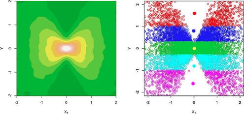
Figure 1: Left panel: contour plot for the joint distribution of $Y$ and $X_{1}$ in example (2). Right panel: conditional means (round dots marks) of $X_{1}$ given slices of $Y$. Slices are indicated by different colors. The corresponding conditional variances of $X_{1}$ are (top to bottom): $2.29$, $0.92$, $0.41$, $0.98$ and $2.33$, respectively.

The SIRI algorithm. Observations are $\{(\mathbf{x}_{i},y_{i})\}_{i=1}^{n}$, where $\mathbf{x}_{i}$ is a $p$-dimensional continuous predictor vector and $y_{i}$ is a univariate response.

• We divide the range of $\{y_{i}\}_{i=1}^{n}$ into $H$ nonoverlapping intervals (or “slices”) $S_{1},\ldots,S_{H}$, with $n_{h}$, the number of observations in $S_{h}$, roughly the same for $h=1,\ldots,H$.

• Let $\mathcal{C}$ denote the set of predictors that have been selected as relevant. Then, for a new candidate variable $X_{j}$ not in $\mathcal{C}$, we compute

  $$\widehat{D}^{*}_{j|\mathcal{C}}=\log\widehat{\sigma}^{2}_{j|\mathcal{C}}-\sum_{h=1}^{H}\frac{n_{h}}{n}\log\bigl{[}\widehat{\sigma}^{(h)}_{j|\mathcal{C}}\bigr{]}^{2},$$

  where $[\widehat{\sigma}^{(h)}_{j|\mathcal{C}}]^{2}$ is the estimated error variance by regressing $X_{j}$ on $\mathbf{X}_{\mathcal{C}}$ in the $h$th slice, and $\widehat{\sigma}^{2}_{j|\mathcal{C}}$ is the estimated error variance by regressing $X_{j}$ on $\mathbf{X}_{\mathcal{C}}$ using all the observations. Variable $X_{j}$ is added to $\mathcal{C}$ if $\widehat{D}^{*}_{j|\mathcal{C}}$ is sufficiently large, and ignored otherwise.

• Each variable within $\mathcal{C}$ is reexamined using the $\widehat{D}^{*}$ statistic for possible removal.

• The above two steps are repeated until no more variables can be added to or removed from $\mathcal{C}$.

Note that one always starts SIRI with $\mathcal{C}=\varnothing$, in which case $\widehat{D}^{*}_{j|\mathcal{C}}$ is reduced to a contrast of the within-slice versus between-slice variances: $\widehat{D}^{*}_{j}=\log\widehat{\sigma}^{2}_{j}-\sum_{h=1}^{H}(n_{h}/n)\log[\widehat{\sigma}^{(h)}_{j}]^{2}$. This test statistic can be used as a sure independence screening criterion when $p$ is extremely large to reduce the set of candidate predictors. The full recursive SIRI procedure based $\widehat{D}^{*}_{j|\mathcal{C}}$ can then be applied to the reduced set of variables.

To illustrate, we generated $200$ observations from example (2) and divided the range of $y$ into $5$ slices with $40$ observations in each slice, that is, $p=1000$, $H=5$, $n=200$ and $n_{h}=40$. We found that $(n\widehat{D}^{*}_{1})=62.48$ and $(n\widehat{D}^{*}_{2})=56.03$ are highly significant compared with their null distributions, which will be shown to be asymptotically $\chi^{2}(8)$ [empirically we observed that $\max_{j\in\{3,4,\ldots,1000\}}(n\widehat{D}^{*}_{j})=28.46$]. So both $X_{1}$ and $X_{2}$ can be easily detected from the screening stage. We also tested whether $X_{2}$ can be correctly selected conditioning on $X_{1}$ by calculating $(n\widehat{D}^{*}_{2|\{1\}})=148.83$. This is also highly significant compared to its null distribution, which is asymptotically $\chi^{2}(12)$ [or to contrast with $\max_{j\in\{3,4,\ldots,1000\}}(n\widehat{D}^{*}_{j|\{1\}})=31.85$]. We were thus able to detect both $X_{1}$ and $X_{2}$ with a computational complexity of $O(p)$.

Note that our main goal here is to select relevant predictors without explicitly stating analytic forms through which they influence $y$. We leave the construction of a specific parametric form to downstream analysis, which can be applied to a small number of selected predictors. For example, to pinpoint the specific interaction term $X_{1}X_{2}$ in example (2), one can apply linear-model based methods to an expanded set of predictors that includes multiplicative interactions between selected variables $\{X_{1},X_{2}\}$.

1.3 Related work

There has been considerable effort in fitting models with interactions and other nonlinear effects in recent statistical literatures. For example, Ravikumar et al. (2009) introduced SpAM (sparse additive nonparametric regression model) that generalizes sparse linear models to the additive, nonparametric setting. Bien, Taylor and Tibshirani (2013) developed hierNet, an extension of Lasso to consider interactions in a model if one or both variables are marginally important (referred to as hierarchical interactions by the authors). Li, Zhong and Zhu (2012) proposed a sure independence screening procedure based on distance correlation (DC-SIS) that is shown to be capable of detecting important variables when interactions are presented.

The inverse modeling perspective that motivates this paper has been taken by several researchers and has led to new developments in dimension reduction and variable selection methods. Cook (2007) proposed inverse regression models for dimension reduction, which have deep connections with the SIR method. Simon and Tibshirani (2012) proposed a permutation-based method for testing interactions by exploring the connection between the forward logistic model and the inverse normal mixture model when the response $Y$ is binary. Another classical method derived from the inverse modeling perspective is the naïve Bayes classifier for classifications with high dimensional features. Although Naïve Bayes classifier is limited by its strong independence assumption, it can be generalized by modeling the joint distribution of features. Murphy, Dean and Raftery (2010) proposed a variable selection method using Bayesian information criterion (BIC) for model-based discriminant analysis. Zhang and Liu (2007) proposed a Bayesian method called BEAM to detect epistatic interactions in genome-wide case–control studies, where $Y$ is binary and the $\mathbf{X}$ are discrete.

The rest of the article is organized as follows. At the beginning of Section 2, we introduce an inverse model of predictors given slices of response and explore its link with SIR. A likelihood-ratio test statistic for selecting relevant predictors under this model is derived in Section 2.1, which is shown to be asymptotically equivalent to the COP statistic in Zhong et al. (2012). We augment the inverse model to detect predictors with second-order effects in Section 2.2. A sure independence screening criterion based on the augmented model is proposed in Section 2.3. A few theoretical results regarding selection consistency of the proposed methods are described in Section 3. By cross-stitching independence screening and likelihood-ratio tests, an iterative stepwise procedure that we referred to as SIRI is developed in Section 4. Various implementation issues including the choices of slicing schemes and thresholds are also discussed. Simulations and real data examples are reported in Sections 5 and 6. Additional remarks in Section 7 conclude the paper. Proofs of the theorems are provided in the Appendix.

2 Variable selection via a sliced inverse model

Let $Y\in\mathbb{R}$ be a univariate response variable and $\mathbf{X}=(X_{1},X_{2},\ldots,X_{p})^{T}\in\mathbb{R}^{p}$ be a vector of $p$ continuous predictor variables. Let $\{(\mathbf{x}_{i},y_{i})\}_{i=1}^{n}$ denote $n$ independent observations on $(\mathbf{X},Y)$. For discrete responses, the $y_{i}$’s can be naturally grouped into a finite number of classes. For continuous responses, we divide the range of $\{y_{i}\}_{i=1}^{n}$ into $H$ disjoint intervals $S_{1},\ldots,S_{H}$, also known as “slices.” Let $S(Y)$ indicate the slice membership of response $Y$, that is, $S(Y)=h$ if $Y\in S_{h}$. For a fixed slicing scheme, we denote $n_{h}=|S_{h}|\equiv ns_{h}$ where $\sum_{h=1}^{H}s_{h}=1$.

To view SIR from a likelihood perspective, we start with a seemingly different model. We assume that the distribution of predictors given the sliced response is multivariate normal:

$$\mathbf{X}|Y\in S_{h}\sim\operatorname{MVN}(\mu_{h},\Sigma),\qquad 1\leq h\leq H,$$ (3)

where $\mu_{h}\in\mu+\mathbb{V}^{q}$ belongs to a $q$-dimensional affine space, $\mathbb{V}^{q}$ is a $q$-dimensional subspace ($q<p$) and $\mu\in\mathbb{R}^{p}$. Alternatively, we can write $\mu_{h}=\mu+\Gamma\gamma_{h}$, where $\gamma_{h}\in\mathbb{R}^{q}$ and $\Gamma$ is a $p$ by $q$ matrix whose columns form a basis of the subspace $\mathbb{V}^{q}$. Although this representation is only unique up to an orthogonal transformation on the bases $\Gamma$, the subspace $\mathbb{V}^{q}$ is unique and identifiable. The following proposition proved by Szretter and Yohai (2009) links the inverse model (3) with SIR.

Proposition 1.

The maximum likelihood estimate (MLE) of the subspace $\mathbb{V}^{q}$ in model (3) coincides with the subspace spanned by SDR directions estimated from the SIR algorithm.

2.1 Likelihood-ratio tests for detecting variables with mean effects

For the purpose of variable selection, we partition predictors into two subsets: a set of relevant predictors indexed by $\mathcal{A}$ and a set of redundant predictors indexed by $\mathcal{A}^{c}$, and assume the following model:

$$\mathbf{X}_{\mathcal{A}}|Y\in S_{h} \sim \operatorname{MVN}\bigl{(}\mu_{h}\in\mu+\mathbb{V}^{q},\Sigma\bigr{)},$$

$$\mathbf{X}_{\mathcal{A}^{c}}|\mathbf{X}_{\mathcal{A}},Y\in S_{h} \sim \operatorname{MVN}\bigl{(}\alpha+\bolds\beta^{T}\mathbf{X}_{\mathcal{A}},\Sigma_{0}\bigr{)}.$$

That is, we assume that the conditional distribution of relevant predictors follows the inverse model (3) of SIR and has a common covariance matrix in different slices. Given the current set of selected predictors indexed by $\mathcal{C}$ with dimension $d$ and another predictor indexed by $j\notin\mathcal{C}$, we propose the following hypotheses:

$$H_{0}\dvtx\mathcal{A}=\mathcal{C}\quad\mbox{v.s.}\quad H_{1}\dvtx\mathcal{A}=\mathcal{C}\cup\{j\}.$$

Let $L_{j|\mathcal{C}}$ denote the likelihood-ratio test statistic for testing $H_{1}$ against $H_{0}$. In Jiang and Liu (2014), we showed that the scaled log-likelihood-ratio test statistic is given by

$$\widehat{D}_{j|\mathcal{C}}=\frac{2}{n}\log(L_{j|\mathcal{C}})=\sum_{k=1}^{q}\log\biggl{(}1+{\frac{\widehat{\lambda}^{d+1}_{k}-\widehat{\lambda}^{d}_{k}}{1-\widehat{\lambda}^{d+1}_{k}}}\biggr{)},$$ (5)

where $\widehat{\lambda}^{d}_{k}$ and $\widehat{\lambda}^{d+1}_{k}$ are estimates of the $k$th profile-$R^{2}$ based on $\mathbf{x}_{\mathcal{C}}$ and $\mathbf{x}_{\mathcal{C}\cup\{j\}}$, respectively. Since ${\frac{\widehat{\lambda}^{d+1}_{k}-\widehat{\lambda}^{d}_{k}}{1-\widehat{\lambda}^{d+1}_{k}}}\mathop{\rightarrow}\limits^{P}0$ as $n\rightarrow\infty$ under $H_{0}$ and that $\log(1+t)=t+O(t^{2})$, we have

$$2\log(L_{j|\mathcal{C}})=(n\widehat{D}_{j|\mathcal{C}})=n\sum_{k=1}^{q}\frac{\widehat{\lambda}^{d+1}_{k}-\widehat{\lambda}^{d}_{k}}{1-\widehat{\lambda}^{d+1}_{k}}+o_{p}(1)\mathop{\rightarrow}\limits^{d}\chi^{2}(q).$$

This expression coincides with the COP statistics proposed by Zhong et al. (2012), which are defined as

$$\operatorname{COP}^{d+1}_{k}=n\frac{\widehat{\lambda}^{d+1}_{k}-\widehat{\lambda}^{d}_{k}}{1-\widehat{\lambda}^{d+1}_{k}},\qquad k=1,2,\ldots,q\quad\mbox{and}\quad\operatorname{COP}^{d+1}_{1\dvtx q}=\sum_{k=1}^{q}\operatorname{COP}^{d+1}_{k}.$$

For all the predictors indexed by $j\in\mathcal{C}^{c}$, we can also obtain the asymptotic joint distribution of $2\log(L_{j|\mathcal{C}})=(n\widehat{D}_{j|\mathcal{C}})$ under the null hypothesis with fixed number of predictors $p$ and as $n\rightarrow\infty$,

$$2\log(L_{j|\mathcal{C}})=(n\widehat{D}_{j|\mathcal{C}})_{j\in\mathcal{C}^{c}}\mathop{\rightarrow}\limits^{d}\Biggl{(}\sum_{k=1}^{q}z^{2}_{kj}\Biggr{)}_{j\in\mathcal{C}^{c}},$$ (6)

where $\mathbf{z}_{k}=(z_{kj})_{j\in\mathcal{C}^{c}}\sim\operatorname{MVN}(\mathbf{0},[\operatorname{Corr}(X_{i},X_{j}|\mathbf{X}_{\mathcal{C}})]_{i,j\in\mathcal{C}^{c}})$ and $\mathbf{z}_{k}$’s are independent. Furthermore, we can show that, as $n\rightarrow\infty$,

$$\widehat{D}_{j|\mathcal{C}} \mathop{\rightarrow}\limits^{\mathrm{a.s.}} D_{j|\mathcal{C}}$$

$$= \log\biggl{(}1+\frac{{\operatorname{Var}(M_{j})-\operatorname{Cov}(M_{j},\mathbf{X}_{\mathcal{C}})[\operatorname{Cov}(\mathbf{X}_{\mathcal{C}})]^{-1}\operatorname{Cov}(M_{j},\mathbf{X}_{\mathcal{C}})^{T}}}{\mathbb{E}(V_{j})}\biggr{)},$$

where $M_{j}=\mathbb{E}(X_{j}|\mathbf{X}_{\mathcal{C}},S(Y))$, $V_{j}=\operatorname{Var}(X_{j}|\mathbf{X}_{\mathcal{C}},S(Y))$ and $S(Y)=h$ when $Y\in S_{h}$ ($1\leq h\leq H)$. By the Cauchy–Schwarz inequality and the normality assumption,

$$D_{j|\mathcal{C}}=0\quad\mathrm{iff}\quad\mathbb{E}(X_{j}|\mathbf{X}_{\mathcal{C}},Y\in S_{h})=\mathbb{E}(X_{j}|\mathbf{X}_{\mathcal{C}}),\qquad 1\leq h\leq H.$$

That is, the test statistic $\widehat{D}_{j|\mathcal{C}}$ almost surely converges to zero if the conditional mean of $X_{j}$ is independent of slice membership $S(Y)$. See Jiang and Liu (2014) for detailed proofs about properties of $\widehat{D}_{j|\mathcal{C}}$.

Given thresholds $\nu_{a}>\nu_{d}$ and the current set of selected predictors indexed by $\mathcal{C}$, we can select relevant variables by iterating the following steps until no new addition or deletion occurs:

• Addition step: find $j_{a}$ such that $\widehat{D}_{j_{a}|\mathcal{C}}=\max_{j\in\mathcal{C}^{c}}\widehat{D}_{j|\mathcal{C}}$; let $\mathcal{C}=\mathcal{C}+\{j_{a}\}$ if $\widehat{D}_{j_{a}|\mathcal{C}}>\nu_{a}$.

• Deletion step: find $j_{d}$ such that $\widehat{D}_{j_{d}|\mathcal{C}-\{j_{d}\}}=\min_{j\in\mathcal{C}}\widehat{D}_{j|\mathcal{C}-\{j\}}$; let $\mathcal{C}=\mathcal{C}-\{j_{d}\}$ if $\widehat{D}_{j_{d}|\mathcal{C}-\{j_{d}\}}<\nu_{d}$.

In Section 3.1, we will study the selection consistency of the foregoing procedure under model (2.1), allowing for the number of predictors $p$ to grow with the sample size $n$.

2.2 Detecting variables with second-order effects

Let us revisit example (2). As illustrated in Figure 1, we have $\mathbb{E}(X_{j}|Y\in S_{h})=0$ for $j=1,2$ and $1\leq h\leq H$. Starting with $\mathcal{C}=\varnothing$, the stepwise procedure in Section 2.1 fails to capture either $X_{1}$ or $X_{2}$ since $D_{1|\mathcal{C}=\varnothing}=D_{2|\mathcal{C}=\varnothing}=0$. In order to detect predictors with different (conditional) variances across slices, such as $X_{1}$ and $X_{2}$ in this example, we augment model (2.1) to a more general form,

$$\mathbf{X}_{\mathcal{A}}|Y\in S_{h} \sim \operatorname{MVN}(\mu_{h},\Sigma_{h}),$$

$$\mathbf{X}_{\mathcal{A}^{c}}|\mathbf{X}_{\mathcal{A}},Y\in S_{h} \sim \operatorname{MVN}\bigl{(}\alpha+\bolds\beta^{T}\mathbf{X}_{\mathcal{A}},\Sigma_{0}\bigr{)},$$

which differs from model (2.1) in its allowing for slice-dependent means and covariance matrices for relevant predictors. To guarantee identifiability, variables indexed by $\mathcal{A}$ in model (2.2) have to be minimally relevant, that is, $\mathcal{A}$ does not contain any predictor that is conditionally independent of $Y$ given the remaining predictors in $\mathcal{A}$. Jiang and Liu (2014) gave a rigorous proof of the uniqueness of minimally relevant predictor set $\mathcal{A}$.

By following the same hypothesis testing framework as in Section 2.1, we can derive the scaled log-likelihood-ratio test statistic under the augmented model (2.2):

$$\widehat{D}^{*}_{j|\mathcal{C}}=\log\widehat{\sigma}^{2}_{j|\mathcal{C}}-\sum_{h=1}^{H}\frac{n_{h}}{n}\log\bigl{[}\widehat{\sigma}^{(h)}_{j|\mathcal{C}}\bigr{]}^{2},$$ (8)

where $\mathcal{C}$ is the set of currently selected predictors and $j\in\mathcal{C}^{c}$, $[\widehat{\sigma}^{(h)}_{j|\mathcal{C}}]^{2}$ is the estimated variance by regressing $X_{j}$ on $\mathbf{X}_{\mathcal{C}}$ in slice $S_{h}$, and $\widehat{\sigma}^{2}_{j|\mathcal{C}}$ is the estimated variance by regressing $X_{j}$ on $\mathbf{X}_{\mathcal{C}}$ using all the observations. Although model (2.2) involves more parameters than model (2.1), by relaxing the homoscedastic constraint on the distribution of relevant predictors across slices, the form of the likelihood-ratio test statistic in (8) appears simpler than that in (5). The augmented test statistic $(n\widehat{D}^{*}_{j|\mathcal{C}})$ was used to select relevant predictors in the illustrative example of Section 1.2.

Under the assumption that $\mathcal{A}\subset\mathcal{C}$ with $|\mathcal{C}|=d$, we can derive the exact and asymptotic distribution of $(n\widehat{D}^{*}_{j|\mathcal{C}})$:

$$n\widehat{D}^{*}_{j|\mathcal{C}} \sim n\log\biggl{(}1+\frac{Q_{0}}{\sum_{h=1}^{H}Q_{h}}\biggr{)}-\sum_{h=1}^{H}\frac{n_{h}}{n}\log\biggl{(}\frac{Q_{h}/n_{h}}{\sum_{h=1}^{H}Q_{h}/n}\biggr{)}$$

$$\mathop{\rightarrow}\limits^{d} \chi^{2}\bigl{(}(H-1)(d+2)\bigr{)},$$

where $Q_{0}\sim\chi^{2}((H-1)(d+1))$ and $Q_{h}\sim\chi^{2}(n_{h}-(d+1))$ ($1\leq h\leq H$) are mutually independent according to Cochran’s theorem. For all the predictors indexed by $j\in\mathcal{C}^{c}$, we can also obtain the asymptotic joint distribution of $(n\widehat{D}^{*}_{j|\mathcal{C}})$ under the assumption that $\mathcal{A}\subset\mathcal{C}$ (with $p$ fixed and $n\rightarrow\infty$):

$$\bigl{(}n\widehat{D}^{*}_{j|\mathcal{C}}\bigr{)}_{j\in\mathcal{C}^{c}}\mathop{\rightarrow}\limits^{d}\Biggl{(}\sum_{i=1}^{(H-1)(d+1)}z^{2}_{ij}+\sum_{i=1}^{H-1}\widetilde{z}^{2}_{ij}\Biggr{)}_{j\in\mathcal{C}^{c}},$$ (9)

where $\mathbf{z}_{i}$’s and $\widetilde{\mathbf{z}}_{i}$’s are mutually independent with

$$\mathbf{z}_{i}=(z_{ij})_{j\in\mathcal{C}^{c}}\sim\operatorname{MVN}\bigl{(}\mathbf{0},\bigl{[}\operatorname{Corr}(X_{j},X_{k}|\mathbf{X}_{\mathcal{C}})\bigr{]}_{j,k\in\mathcal{C}^{c}}\bigr{)}$$

and

$$\widetilde{\mathbf{z}}_{i}=(\widetilde{z}_{ij})_{j\in\mathcal{C}^{c}}\sim\operatorname{MVN}\bigl{(}\mathbf{0},\bigl{[}\operatorname{Corr}^{2}(X_{j},X_{k}|\mathbf{X}_{\mathcal{C}})\bigr{]}_{j,k\in\mathcal{C}^{c}}\bigr{)}.$$

When the number of predictors $p$ is fixed and the sample size $n\rightarrow\infty$,

$$\widehat{D}^{*}_{j|\mathcal{C}} \mathop{\rightarrow}\limits^{\mathrm{a.s.}} D^{*}_{j|\mathcal{C}}$$

$$= \log\biggl{(}1+\frac{{\operatorname{Var}(M_{j})-\operatorname{Cov}(M_{j},\mathbf{X}_{\mathcal{C}})[\operatorname{Cov}(\mathbf{X}_{\mathcal{C}})]^{-1}\operatorname{Cov}(M_{j},\mathbf{X}_{\mathcal{C}})^{T}}}{\mathbb{E}(V_{j})}\biggr{)}$$

$${}+\log\mathbb{E}(V_{j})-\mathbb{E}\log(V_{j}),$$

where $M_{j}=\mathbb{E}(X_{j}|\mathbf{X}_{\mathcal{C}},S(Y))$, $V_{j}=\operatorname{Var}(X_{j}|\mathbf{X}_{\mathcal{C}},S(Y))$ and $S(Y)=h$ when $Y\in S_{h}$ ($1\leq h\leq H$). According to the Cauchy–Schwarz inequality and Jensen’s inequality,

$$D^{*}_{j|\mathcal{C}}=0 \quad\mbox{iff}\quad\mathbb{E}(X_{j}|\mathbf{X}_{\mathcal{C}},Y\in S_{h})=\mathbb{E}(X_{j}|\mathbf{X}_{\mathcal{C}})\quad\mbox{and}$$

$$\qquad\operatorname{Var}(X_{j}|\mathbf{X}_{\mathcal{C}},Y\in S_{h})=\operatorname{Var}(X_{j}|\mathbf{X}_{\mathcal{C}}),$$

for $1\leq h\leq H$. That is, the augmented test statistic $\widehat{D}^{*}_{j|\mathcal{C}}$ almost surely converges to zero if both the conditional mean and the conditional variance of $X_{j}$ is independent of slice membership $S(Y)$. Detailed proofs of these properties are collected in Jiang and Liu (2014).

A forward-addition backward-deletion algorithm similar to the stepwise procedure proposed in Section 2.1 can be used with the augmented likelihood-ratio test statistic $\widehat{D}^{*}_{j|\mathcal{C}}$. In Section 3.2, we will provide theoretical results on the selection consistency of stepwise procedure based on $\widehat{D}^{*}_{j|\mathcal{C}}$.

2.3 Sure independence screening strategy: SIS^∗

When dimensionality $p$ is very large, the performance of the stepwise procedure can be compromised. We recommend adding an independence screening step to first reduce the dimensionality from ultra-high to moderately high. A natural choice of the test statistic for the independence screening procedure is $\widehat{D}^{*}_{j|\mathcal{C}}$ with $\mathcal{C}=\varnothing$, that is,

$$\widehat{D}^{*}_{j}=\log\widehat{\sigma}^{2}_{j}-\sum_{h=1}^{H}\frac{n_{h}}{n}\log\bigl{[}\widehat{\sigma}^{(h)}_{j}\bigr{]}^{2},$$

where $[\widehat{\sigma}^{(h)}_{j}]^{2}$ is the estimated variance of $X_{j}$ in slice $S_{h}$, and $\widehat{\sigma}^{2}_{j}$ is the estimated variance of $X_{j}$ using all the observations. In Section 3.3, we will show that if we rank predictors according to $\{\widehat{D}^{*}_{j},1\leq j\leq p\}$, then the sure independence screening procedure, which we call SIS^∗, that takes the first $o(n)$ predictors has a high probability (almost surely) of including relevant predictors that have either different means or different variances across slices.

3 Theoretical results

We here establish the selection consistency for procedures introduced in Sections 2.1 and 2.2, as well as the SIS^∗ screening strategy in Section 2.3.

3.1 Selection consistency under homoscedastic model

To proceed, we need the following concept to study the detectability of relevant predictors under model (2.1).

Definition 1 ((First-order detectable)).

We say a collection of predictors indexed by $\mathcal{C}_{0}$ is first-order detectable if there exist $\kappa\geq 0$ and $\xi_{0}>0$ such that for any set of predictors indexed by $\mathcal{C}$ and $\mathcal{C}^{c}\cap\mathcal{C}_{0}\neq\varnothing$,

$$\max_{j\in\mathcal{C}^{c}\cap\mathcal{C}_{0}}\biggl{[}\frac{\operatorname{Var}(M_{j})-\operatorname{Cov}(M_{j},\mathbf{X}_{\mathcal{C}})[\operatorname{Cov}(\mathbf{X}_{\mathcal{C}})]^{-1}\operatorname{Cov}(M_{j},\mathbf{X}_{\mathcal{C}})^{T}}{\mathbb{E}(V_{j})}\biggr{]}\geq\xi_{0}n^{-\kappa},$$

where $M_{j}=\mathbb{E}(X_{j}|\mathbf{X}_{\mathcal{C}},S(Y))$ and $V_{j}=\operatorname{Var}(X_{j}|\mathbf{X}_{\mathcal{C}},S(Y))$.

In the above definition, we allow the distribution of the random samples $(\mathbf{X},Y)$ to be dependent on the sample size $n$. For any first-order detectable predictor, its conditional means given other predictors and different slices are not all identical and differences among these conditional means are not too small relative to the sample size. The following example illustrates the implication of Definition 1.

Example 1.

Suppose $Y$ is divided into two slices and there are two predictors $(X_{1},X_{2})$. Conditional distributions of the $X$ given the slices are

$$\pmatrix{X_{1}\vspace*{2pt}\cr X_{2}}\bigg{|}Y\in S_{1} \sim \operatorname{MVN}\biggl{(}\pmatrix{1\vspace*{2pt}\cr 1},\pmatrix{1&1\vspace*{2pt}\cr 1&2}\biggr{)}\quad\mbox{and}$$

$$\pmatrix{X_{1}\vspace*{2pt}\cr X_{2}}\bigg{|}Y\in S_{2} \sim \operatorname{MVN}\biggl{(}\pmatrix{-1\vspace*{2pt}\cr-1},\pmatrix{\sigma^{2}&\sigma^{2}\vspace*{2pt}\cr\sigma^{2}&2\sigma^{2}}\biggr{)}.$$

It is easy to show that $X_{1}$ is first-order detectable but $X_{2}$ is not because $\mathbb{E}(X_{2}|X_{1},Y\in S_{h})=X_{1}$, which is identical for $h=1,2$. If $\sigma^{2}=1$, $X_{2}$ and $Y$ are conditionally independent given $X_{1}$, and $X_{2}$ is indeed redundant for predicting $Y$ if we have already included $X_{1}$. If $\sigma^{2}\neq 1$, however, $\operatorname{Var}(X_{2}|X_{1},Y\in S_{h})$ depends on $h$, and thus, $X_{2}$ is relevant for predicting $Y$ even if we have included $X_{1}$. However, procedures that can only detect first-order detectable predictors will miss $X_{2}$ in this case.

Suppose the following conditions hold for predictors $\mathbf{X}$ with dimension $p$.

Condition 1.

There exist $0<\tau_{\mathrm{min}}<\tau_{\mathrm{max}}<\infty$ such that

$$\tau_{\mathrm{min}}\leq\lambda_{\mathrm{min}}\bigl{(}\operatorname{Cov}(\mathbf{X}|Y\in S_{h})\bigr{)}<\lambda_{\mathrm{max}}\bigl{(}\operatorname{Cov}(\mathbf{X}|Y\in S_{h})\bigr{)}\leq\tau_{\mathrm{max}},$$

and that

$$\lambda_{\mathrm{max}}\bigl{(}\operatorname{Cov}(\mathbf{X})\bigr{)}\leq\tau_{\mathrm{max}},$$

where $\lambda_{\mathrm{min}}(\cdot)$ and $\lambda_{\mathrm{max}}(\cdot)$ denote the smallest and largest eigenvalues, respectively, of a positive definite matrix.

Condition 2.

$p=O(n^{\rho})$ as $n\rightarrow\infty$ with $\rho>0$ and $2\rho+2\kappa<1$, where $\kappa$ is the same constant as in Definition 1.

Condition 1 excludes singular cases when some predictors are constants or highly correlated. Assuming that Condition 1 holds, Jiang and Liu (2014) gave an equivalent characterization of first-order detectable predictors under model (2.1). Condition 2 allows the number of predictors $p$ to grow with the sample size $n$ but the growth rate cannot exceed $n^{{1}/{2}-\kappa}$. In situations when $p$ is larger than $n^{{1}/{2}-\kappa}$, we can first use the screening strategy SIS^∗ introduced in Section 2.3 to reduce the dimensionality. In Section 3.3, we will show theoretically that SIS^∗ can be used to deal with scenarios when $p$ is much larger than $n$. The following theorem, which is proved in Appendix .1, guarantees that the stepwise procedure described in Section 2.1 is selection consistent for first-order detectable predictors if two thresholds $\nu_{a}$ and $\nu_{d}$ are chosen appropriately.

Theorem 1.

Under model (2.1), Conditions 1 and 2, if the set of relevant predictors indexed by $\mathcal{A}$ is first-order detectable with constant $\kappa$, then there exists constant $c>0$ such that

$$\operatorname{Pr}\Bigl{(}\min_{\mathcal{C}\dvtx\mathcal{C}^{c}\cap\mathcal{A}\neq\varnothing}\max_{j\in\mathcal{C}^{c}}\widehat{D}_{j|\mathcal{C}}\geq cn^{-\kappa}\Bigr{)}$$

$$\qquad\geq 1-O\biggl{(}p(p+1)q\exp{\biggl{(}-N_{1}\frac{n^{1-2\kappa}}{p^{2}q^{2}}\biggr{)}}\biggr{)}\rightarrow 1$$

and

$$\operatorname{Pr}\biggl{(}\max_{\mathcal{C}\dvtx\mathcal{C}^{c}\cap\mathcal{A}=\varnothing}\max_{j\in\mathcal{C}^{c}}\widehat{D}_{j|\mathcal{C}}<\frac{c}{2}n^{-\kappa}\biggr{)}$$

$$\qquad\geq 1-O\biggl{(}p(p+1)q\exp{\biggl{(}-N_{2}\frac{n^{1-2\kappa}}{p^{2}q^{2}}\biggr{)}}\biggr{)}\rightarrow 1,$$

as $n\rightarrow\infty$, where $N_{1}$ and $N_{2}$ are positive constants.

The first convergence result implies that as long as the set of currently selected predictors $\mathcal{C}$ does not contain all relevant predictors in $\mathcal{A}$, that is, $\mathcal{C}^{c}\cap\mathcal{A}\neq\varnothing$, with probability going to $1$ ($n\rightarrow\infty$) we can find a predictor $j\in\mathcal{C}^{c}$ such that the test statistic $\widehat{D}_{j|\mathcal{C}}\geq cn^{-\kappa}$. Thus, if we choose the threshold $\nu_{a}=cn^{-\kappa}$ in the stepwise procedure, the addition step will not stop selecting variables until all relevant predictors have been included. On the other hand, once all relevant predictors have been included in $\mathcal{C}$, that is, $\mathcal{C}^{c}\cap\mathcal{A}=\varnothing$, the second result guarantees that, with probability going to $1$, $\widehat{D}_{j|\mathcal{C}}<(c/2)n^{-\kappa}<\nu_{a}$ for any predictor $j\in\mathcal{C}^{c}$. Thus, the addition step will stop selecting other predictors into $\mathcal{C}$. Consequently, if we choose $\nu_{d}=(c/2)n^{-\kappa}$ in the deletion step, then all redundant variables will be removed from the set of selected variables until $\mathcal{C}=\mathcal{A}$ as $n\rightarrow\infty$.

3.2 Selection consistency under augmented model

Under model (2.2), we can further extend the definition of detectability to include predictors with interactions and other second-order effects.

Definition 2 ((Second-order detectable)).

We call a collection of predictors indexed by $\mathcal{C}_{2}$ second-order detectable given predictors indexed by $\mathcal{C}_{1}$ if $\mathcal{C}_{2}\cap\mathcal{C}_{1}=\varnothing$, and for any set $\mathcal{C}$ satisfying $\mathcal{C}_{1}\subset\mathcal{C}$ and $\mathcal{C}_{2}\not\subset\mathcal{C}$, there exist constants $\xi_{1},\xi_{2}>0$ and $\kappa\geq 0$ such that either

$$\max_{j\in\mathcal{C}^{c}\cap\mathcal{C}_{2}}\biggl{[}\frac{\operatorname{Var}(M_{j})-\operatorname{Cov}(M_{j},\mathbf{X}_{\mathcal{C}})[\operatorname{Cov}(\mathbf{X}_{\mathcal{C}})]^{-1}\operatorname{Cov}(M_{j},\mathbf{X}_{\mathcal{C}})^{T}}{\mathbb{E}(V_{j})}\biggr{]}\geq\xi_{1}n^{-\kappa},$$ (10)

or

$$\max_{j\in\mathcal{C}^{c}\cap\mathcal{C}_{2}}\bigl{[}\log(\mathbb{E}V_{j})-\mathbb{E}\log(V_{j})\bigr{]}\geq\xi_{2}n^{-\kappa},$$

where $M_{j}=\mathbb{E}(X_{j}|\mathbf{X}_{\mathcal{C}},S(Y))$, $V_{j}=\operatorname{Var}(X_{j}|\mathbf{X}_{\mathcal{C}},S(Y))$.

In other words, if the current selection $\mathcal{C}$ contains $\mathcal{C}_{1}$, then there always exist detectable predictors conditioning on currently selected variables until we include all the predictors indexed by $\mathcal{C}_{2}$. A relevant predictor $X_{j}$ indexed by $j\notin\mathcal{C}_{2}$ is not second-order detectable given $\mathcal{C}_{1}$ either because it is highly correlated with some other predictors, or its effect can only be detected when conditioning on predictors that have not been included in $\mathcal{C}_{1}$. Based on Definition 2, we define stepwise detectable as follows.

Definition 3 ((Stepwise detectable)).

A collection of predictors indexed by $\mathcal{T}_{0}$ is said to be $0$-stage detectable if $\mathbf{X}_{\mathcal{T}_{0}}$ is second-order detectable conditioning on an empty set, and a collection of predictors indexed by $\mathcal{T}_{m}$ is said to be $m$-stage detectable ($m\geq 1$) if $\mathbf{X}_{\mathcal{T}_{m}}$ is second-order detectable given predictors indexed by $\bigcup_{i=1}^{m-1}\mathcal{T}_{i}$. Finally, a predictor indexed by $j$ is said to be stepwise detectable if $j\in\bigcup_{i=1}^{\infty}\mathcal{T}_{i}$.

According to Definition 1, given the same constant $\kappa$, there exists $\xi_{1}$ such that the set of first-order detectable predictors defined in Definition 1 is contained in the set of stepwise detectable predictors. The following simple example illustrates the usefulness of foregoing definitions.

Example 2.

Suppose $Y$ is divided into two slices and there are only two predictors $(X_{1},X_{2})$. Conditional distributions given the slices are

$$\pmatrix{X_{1}\vspace*{2pt}\cr X_{2}}\bigg{|}Y\in S_{1} \sim \operatorname{MVN}\biggl{(}\pmatrix{0\vspace*{2pt}\cr 0},\pmatrix{\sigma_{1}^{2}&1\vspace*{2pt}\cr 1&1}\biggr{)}\quad\mbox{and}$$

$$\pmatrix{X_{1}\vspace*{2pt}\cr X_{2}}\bigg{|}Y\in S_{2} \sim \operatorname{MVN}\biggl{(}\pmatrix{0\vspace*{2pt}\cr 0},\pmatrix{\sigma_{2}^{2}&-1\vspace*{2pt}\cr-1&1}\biggr{)},$$

where $\sigma_{1}^{2},\sigma_{2}^{2}>1$. When $\sigma_{1}^{2}\neq\sigma_{2}^{2}$ and the sample size $n$ is large enough, $X_{1}$ is $0$-stage second-order detectable (without conditioning on any other predictor), and $X_{2}$ is $1$-stage second-order detectable conditioning on $X_{1}$ because the conditional distribution, $X_{2}|X_{1},Y\in S_{h}\sim\mathrm{N}((-1)^{h+1}X_{1}/\sigma_{h}^{2},1-1/\sigma_{h}^{2})$, is different for $h=1$ and $2$. Thus, both $X_{1}$ and $X_{2}$ are stepwise detectable. When $\sigma_{1}^{2}=\sigma_{2}^{2}$, although $X_{1}$ and $X_{2}$ are relevant predictors since the two conditional distributions are different, none of them are stepwise detectable. In this case, no stepwise procedure that selects one variable at a time is able to “detect” either $X_{1}$ or $X_{2}$.

In Appendix .2, we prove the following theorem, which guarantees that by appropriately choosing thresholds, the stepwise procedure will keep adding predictors until all the stepwise detectable predictors have been included, and keep removing predictors until all the redundant variables have been excluded.

Theorem 2.

Under model (2.2), Conditions 1 and 2, if all the relevant predictors indexed by $\mathcal{A}$ are stepwise detectable with constant $\kappa$, then there exists constant $c^{*}>0$ such that as $n\rightarrow\infty$,

$$\operatorname{Pr}\Bigl{(}\min_{\mathcal{C}\dvtx\mathcal{C}^{c}\cap\mathcal{A}\neq\varnothing}\max_{j\in\mathcal{C}^{c}}\widehat{D}^{*}_{j|\mathcal{C}}\geq c^{*}n^{-\kappa}\Bigr{)}$$

$$\qquad\geq 1-O\biggl{(}p(p+1)(H+1)\exp{\biggl{(}-M_{1}\frac{n^{1-2\kappa}}{p^{2}H^{2}}\biggr{)}}\biggr{)}\rightarrow 1$$

and

$$\operatorname{Pr}\biggl{(}\max_{\mathcal{C}\dvtx\mathcal{C}^{c}\cap\mathcal{A}=\varnothing}\max_{j\in\mathcal{C}^{c}}\widehat{D}^{*}_{j|\mathcal{C}}<\frac{c^{*}}{2}n^{-\kappa}\biggr{)}$$

$$\qquad\geq 1-O\biggl{(}p(p+1)(H+1)\exp{\biggl{(}-M_{2}\frac{n^{1-2\kappa}}{p^{2}H^{2}}\biggr{)}}\biggr{)}\rightarrow 1,$$

where $M_{1}$ and $M_{2}$ are positive constants.

Therefore, by appropriately choosing the thresholds, the stepwise procedure based on $\widehat{D}^{*}_{j|\mathcal{C}}$ is consistent in identifying stepwise detectable predictors.

3.3 Sure independence screening property of SIS^∗

Definition 4 ((Individually detectable)).

We call a predictor $X_{j}$ individually detectable if there exist constants $\xi_{1},\xi_{2}>0$ and $\kappa\geq 0$ such that either

$$\frac{\operatorname{Var}(\mathbb{E}(X_{j}|S(Y)))}{\mathbb{E}(\operatorname{Var}(X_{j}|S(Y)))}\geq\xi_{1}n^{-\kappa},$$ (11)

or

$$\log\mathbb{E}\bigl{(}\operatorname{Var}\bigl{(}X_{j}|S(Y)\bigr{)}\bigr{)}-\mathbb{E}\log\bigl{[}\operatorname{Var}\bigl{(}X_{j}|S(Y)\bigr{)}\bigr{]}\geq\xi_{2}n^{-\kappa}.$$

Simply put, individually detectable predictors have either different means or different variances across slices. Therefore, in the example (2), both $X_{1}$ and $X_{2}$ are individually detectable because $\operatorname{Var}(X_{1}|Y\in S_{h})$ and $\operatorname{Var}(X_{2}|Y\in S_{h})$ ($1\leq h\leq H$) are different across slices. Note that not all stepwise detectable predictors according to Definition 3 are individually detectable. In Example 2 with $\sigma_{1}\neq\sigma_{2}$, $X_{2}$ has the same distribution given $Y\in S_{1}$ or $Y\in S_{2}$, but the conditional distributions of $X_{2}$ given $X_{1}$ are different in two slices. That is, $X_{2}$ is stepwise detectable. However, an independence screening method can only pick up variable $X_{1}$, but not $X_{2}$.

Theorem 3, which is proved in Jiang and Liu (2014), shows that SIS^∗ almost surely includes all the individually detectable predictors under the following condition with ultra-high dimensionality of predictors.

Condition 3.

$\log(p)=O(n^{\gamma})$ as $n\rightarrow\infty$ with $0<\gamma+2\kappa<1$, where $\kappa$ is the same constant as in (11). Furthermore, the number of the relevant predictors $|\mathcal{A}|\leq n^{\eta}$ with $\eta+2\kappa<1/2$.

Theorem 3.

Under Conditions 1 and 3, if all the relevant predictors indexed by $\mathcal{A}$ are individually detectable, then there exist $c>0$ and $C>0$ such that

$$\operatorname{Pr}\Bigl{(}\min_{j\in\mathcal{A}}\widehat{D}^{*}_{j}\geq cn^{-\kappa}\Bigr{)}$$

$$\qquad\geq 1-O\biggl{(}p(H+1)\exp{\biggl{(}-L_{1}\frac{n^{1-2\kappa}}{H^{2}}\biggr{)}}\biggr{)}\rightarrow 1$$

and

$$\operatorname{Pr}\bigl{(}\bigl{|}\bigl{\{}j\dvtx\widehat{D}^{*}_{j}\geq cn^{-\kappa},1\leq j\leq p\bigr{\}}\bigr{|}\leq Cn^{\kappa+\eta}\bigr{)}$$

$$\qquad\geq 1-O\biggl{(}p(H+1)\exp{\biggl{(}-L_{2}\frac{n^{1-2\kappa}}{H^{2}}\biggr{)}}\biggr{)}\rightarrow 1,$$

where $L_{1}$ and $L_{2}$ are positive constants.

According to Theorem 3, we can first use SIS^∗, which is based on $\{\widehat{D}^{*}_{j},1\leq j\leq p\}$, to reduce the dimensionality from $p$ to a scale between $n^{\kappa+\eta}$ and $n^{{1}/{2}-\kappa}$ (since $\eta+\kappa<1/2-\kappa$ under Condition 3), and then apply the stepwise procedure proposed in the previous sections, which is consistent with dimensionality below $n^{{1}/{2}-\kappa}$. As discussed above, predictors that are stepwise detectable according to Definition 3 are not necessarily individually detectable. Fan and Lv (2008) advocated an iterative procedure that alternates between a large-scale screening and a moderate-scale variable selection to enhance the performance, which will be discussed in the next section.

4 Implementation issues: Cross-stitching and cross-validation

The simple model (2.1) and the augmented model (2.2) compensate each other in terms of the bias-variance trade-off. Given finite observations, model (2.1) is simpler and more powerful when the response is driven by some linear combinations of covariates, while model (2.2) is useful in detecting variables with more complex relationships such as heteroscedastic effects or interactions. Similarly, the SIS^∗ procedure introduced in Section 2.3 is very useful when we have a very large number of predictors, but it cannot pick up stepwise detectable predictors that have the same marginal distributions across slices. To find a balance between simplicity and detectability, we propose the following cross-stitching strategy:

• Step 0: initialize the current selection $\mathcal{C}=\varnothing$; rank predictors according to $\{\widehat{D}^{*}_{j},1\leq j\leq p\}$ and select a subset of predictors, denoted as $\mathcal{S}$, using SIS^∗;

• Step 1: select predictors from set $\mathcal{S}\setminus\mathcal{C}$ by using the stepwise procedure with addition and deletion steps based on $\widehat{D}_{j|\mathcal{C}}$ in (5) and add the selected predictors into $\mathcal{C}$;

• Step 2: select predictors from set $\mathcal{S}\setminus\mathcal{C}$ by using the stepwise procedure with addition and deletion steps based on $\widehat{D}^{*}_{j|\mathcal{C}}$ in (8) and add the selected predictors into $\mathcal{C}$;

• Step 3: conditioning on the current selection $\mathcal{C}$, rank the remaining predictors based on $\{\widehat{D}^{*}_{j|\mathcal{C}},j\notin\mathcal{C}\}$, update set $\mathcal{S}$ using SIS^∗, and iterate steps 1–3 until no more predictors are selected.

We name the proposed procedure sliced inverse regression for variable selection via inverse modeling, or SIRI for short. A flowchart of the SIRI procedure is illustrated in Figure 2.

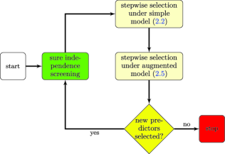
Figure 2: Flowchart of SIRI.

Theoretically, step $2$ is able to detect both linear and more complex relationships and $\widehat{D}^{*}_{j|\mathcal{C}}$ picks up a larger set than $\widehat{D}_{j|\mathcal{C}}$ does. However, in practice, we have to use a relatively large threshold in step 2 to control the number of false positives and thus may falsely discard linear predictors when their effects are weak. Empirically, we have found that adding step 1 will enhance the performance of SIRI in linear or near-linear models, while having almost no effects on its performances in complex models with interaction or other second-order terms.

In the addition step of the stepwise procedure, instead of selecting the variable from $\mathcal{C}^{c}$ with the maximum value of $\widehat{D}_{j|\mathcal{C}}$ (or $\widehat{D}^{*}_{j|\mathcal{C}}$), we may also sequentially add variables with $\widehat{D}_{j|\mathcal{C}}>\nu_{a}$ (or $\widehat{D}^{*}_{j|\mathcal{C}}>\nu_{a}^{*}$). Specifically, given thresholds $\nu_{a}>\nu_{d}$ and the current set of selected predictors indexed by $\mathcal{C}$, we can modify each iteration of the original stepwise procedure as following:

• Modified addition step: for each variable $j\in\{1,\ldots,p\}$, let $\mathcal{C}=\mathcal{C}+\{j\}$ if $j\notin\mathcal{C}$ and $\widehat{D}_{j|\mathcal{C}}>\nu_{a}$.

• Deletion step: find $j_{d}$ such that $\widehat{D}_{j_{d}|\mathcal{C}-\{j_{d}\}}=\min_{j\in\mathcal{C}}\widehat{D}_{j|\mathcal{C}-\{j\}}$; let $\mathcal{C}=\mathcal{C}-\{j_{d}\}$ if $\widehat{D}_{j_{d}|\mathcal{C}-\{j_{d}\}}<\nu_{d}$.

The stepwise procedure with the modified addition step may use fewer iterations to find all relevant predictors and will not stop until all relevant predictors have been included if we choose $\nu_{a}=cn^{-\kappa}$ in Theorem 1. However, in practice, the performance of the modified procedure depends on the ordering of the variables and is less stable than the original procedure. Since we are less concerned about the computational cost of SIRI, we implement the original addition step in the following study.

In our previous discussions, we have assumed that a fixed slicing scheme is given. In practice, we need to choose a slicing scheme. If we assume that there is a true slicing scheme from which data are generated, Jiang and Liu (2014) showed that the power of the stepwise procedure tends to increase with a larger number of slices, but there is no gain by further increasing the number of slices once the slicing is already more refined than the true slicing scheme. In practice, the true slicing scheme is usually unknown (except maybe in cases when the response is discrete). When a slicing scheme uses a larger number of slices, the number of observations in each slice decreases, which makes the estimation of parameters in the model less accurate and less stable. We observed from intensive simulation studies that, with a reasonable number of observations in each slice (say 40 or more), a larger number of slices is preferred.

We also need to choose the number of effective directions $q$ in model (2.1) and thresholds for deciding to add or to delete variables. Sections 2 and 3 characterize asymptotic distributions and behaviors of stepwise procedures, and provide some theoretical guidelines for choosing the thresholds. However, these theoretical results are not directly usable because: (1) the asymptotic distributions that we derived in (6) and (9) are for a single addition or deletion step; (2) the consistency results are valid in asymptotic sense and the rate of increase in dimension relative to sample size is usually unknown. In practice, we propose to use a $K$-fold cross-validation (CV) procedure for selecting thresholds and the number of effective directions $q$.

We consider two performance measures for $K$-fold cross-validations: classification error (CE) and mean absolute error (AE). Suppose there are $n$ training samples and $m$ testing samples. The $j$th observation ($j=1,2,\ldots,m$) in the testing set has response $y_{j}$ and slice membership $S(y_{j})$ (the slicing scheme is fixed based on training samples). Let $p_{j}^{(h)}=\operatorname{Pr}(S(y_{j})=h|\mathbf{X}=\mathbf{x}_{j},\widehat{\theta})$ be the estimated probability that the observation $j$ is from slice $S_{h}$, where $\widehat{\theta}$ denotes the maximum likelihood estimate of model parameters. The classification error is defined as

$$\operatorname{CE}=\frac{1}{m}\sum_{j=1}^{m}\mathbb{I}\Bigl{[}S(y_{j})\neq\mathop{\operatorname{argmax}}_{h}\bigl{(}p_{j}^{(h)}\bigr{)}\Bigr{]}.$$

We denote the average response of training samples in slice $S_{h}$ as

$$\bar{y}^{(h)}=\frac{\sum_{i=1}^{n}\mathbb{I}[S(y_{i})=h]y_{i}}{\sum_{i=1}^{n}\mathbb{I}[S(y_{i})=h]},\qquad h=1,2,\ldots,H.$$

The absolute error is defined as

$$\operatorname{AE}=\frac{1}{m}\sum_{j=1}^{m}\Biggl{|}y_{j}-\sum_{h=1}^{H}p_{j}^{(h)}\bar{y}^{(h)}\Biggr{|}.$$

CE is a more relevant performance measure when the response is categorical or there is a nonsmooth functional relationship (e.g., rational functions) between the response and predictors, and AE is a better measure when there is a monotonic and smooth functional relationship between the response and predictors. There are other measures that have compromising features between these two measures, such as median absolute deviation, which will not be explored here. We will use CE and AE as performance measures throughout simulation studies and name the corresponding methods SIRI-AE and SIRI-CE, respectively.

5 Simulation studies

In order to facilitate fair comparisons with other existing methods that are motivated from the forward modeling perspective, examples presented here are all generated under forward models, which violates the basic model assumption of SIRI. The setting of the simulation also demonstrates the robustness of SIRI when some of its model assumptions are violated, especially the normality assumption on relevant predictor variables within each slice.

5.1 Independence screening performance

We first compare the variable screening performance of SIRI with iterative sure independence screening (ISIS) based on correlation learning proposed by Fan and Lv (2008) and sure independence screening based on distance correlation (DC-SIS) proposed by Li, Zhong and Zhu (2012). We evaluate the performance of each method according to the proportion that relevant predictors are placed among the top $[n/\log(n)]$ predictors ranked by it, with larger values indicating better performance in variable screening.

In the simulation, the predictor variables $\mathbf{X}=(X_{1},X_{2},\ldots,X_{p})^{T}$ were generated from a $p$-variate normal distribution with meanu $0$ and covariances $\operatorname{Cov}(X_{i},X_{j})=\rho^{|i-j|}$ for $1\leq i,j\leq p$. We generate the response variable from the following three scenarios:

$$\mbox{Scenario }0.1\mbox{:}\qquad Y=X_{2}-\rho X_{1}+0.2X_{100}+\sigma\varepsilon,$$

$$\mbox{Scenario }0.2\mbox{:}\qquad Y=X_{1}X_{2}+\sigma e^{2|X_{100}|}\varepsilon,$$

$$\mbox{Scenario }0.3\mbox{:}\qquad Y=\frac{X_{100}}{X_{1}+X_{2}}+\sigma\varepsilon,$$

where sample size $n=200$, $\sigma=0.2$, and $\varepsilon\sim N(0,1)$ independent of $\mathbf{X}$. For each scenario, we simulated $100$ data sets according to six different settings with dimension $p=2000$ or $5000$ and correlation $\rho=0.0$, $0.5$ or $0.9$. Scenario $0.1$ is a linear model with three additive effects. The way $X_{1}$ is introduced is to make it marginally uncorrelated with the response $Y$ (note that when $\rho=0.0$, $X_{1}$ is not a relevant predictor). We added another variable $X_{100}$ that has negligible correlation with $X_{1}$ and $X_{2}$ and a very small correlation with the response $Y$. Scenario $0.2$ contains an interaction term $X_{1}X_{2}$ and a heteroscedatic noise term determined by $X_{100}$. Scenario $0.3$ is an example of a rational model with interactions.

Table 1: The proportions that relevant predictors are placed among the top $[n/\log(n)]$ by different screening methods under Scenarios 0.1–0.3 in Section 5.1

	Scenario 0.1			Scenario 0.2			Scenario 0.3
Method	$\bolds{X_{1}}$	$\bolds{X_{2}}$	$\bolds{X_{100}}$	$\bolds{X_{1}}$	$\bolds{X_{2}}$	$\bolds{X_{100}}$	$\bolds{X_{1}}$	$\bolds{X_{2}}$	$\bolds{X_{100}}$
Setting 1: $p=2000$, $\rho=0.0$
ISIS	–	1.00	1.00	0.02	0.01	0.46	0.00	0.00	0.09
DC-SIS	–	1.00	0.55	0.07	0.09	1.00	0.00	0.00	0.60
SIRI	–	1.00	0.30	0.32	0.25	0.97	1.00	0.99	1.00
Setting 2: $p=2000$, $\rho=0.5$
ISIS	1.00	1.00	1.00	0.04	0.02	0.54	0.00	0.00	0.15
DC-SIS	0.02	1.00	0.71	0.55	0.53	1.00	0.03	0.00	0.59
SIRI	1.00	1.00	0.45	0.92	0.87	0.92	1.00	1.00	1.00
Setting 3: $p=2000$, $\rho=0.9$
ISIS	0.93	0.98	0.91	0.03	0.02	0.55	0.00	0.00	0.04
DC-SIS	0.01	0.99	1.00	0.96	0.95	1.00	0.34	0.38	0.63
SIRI	0.93	0.82	0.79	0.99	0.56	0.95	0.98	0.98	1.00
Setting 4: $p=5000$, $\rho=0.0$
ISIS	–	1.00	1.00	0.02	0.00	0.43	0.00	0.00	0.06
DC-SIS	–	1.00	0.39	0.03	0.05	1.00	0.00	0.00	0.44
SIRI	–	1.00	0.14	0.15	0.16	0.99	0.99	1.00	1.00
Setting 5: $p=5000$, $\rho=0.5$
ISIS	1.00	1.00	1.00	0.03	0.02	0.60	0.00	0.00	0.07
DC-SIS	0.05	1.00	0.71	0.41	0.44	1.00	0.00	0.02	0.61
SIRI	1.00	1.00	0.39	0.88	0.86	0.94	0.98	1.00	0.99
Setting 6: $p=5000$, $\rho=0.9$
ISIS	0.86	0.99	0.87	0.02	0.03	0.34	0.00	0.00	0.03
DC-SIS	0.01	0.99	0.99	0.92	0.93	1.00	0.22	0.13	0.49
SIRI	0.82	0.79	0.74	0.95	0.53	0.90	0.85	0.99	1.00

Proportions that relevant predictors are placed among the top $[n/\log(n)]$ by different screening methods are shown in Table 1. Under Scenario $0.1$ with linear models, we can see that ISIS and DC-SIS had better power than SIRI in detecting variables that are weakly correlated with the response ($X_{100}$ in this example). When predictors are correlated (Settings 2–3 and 4–5), iterative procedures, ISIS and SIRI, were more effective in detecting variables that are marginally uncorrelated with the response ($X_{1}$ in this example) compared with DC-SIS. Under Scenario $0.2$, ISIS based on linear models failed to detect the variables in the interaction term and often misses the predictor in the heteroscedastic noise term. When there are moderate correlations between two predictors $X_{1}$ and $X_{2}$ in the interaction term (Settings $2$ and $4$), DC-SIS picked up $X_{1}$ and $X_{2}$ about half of the time. However, when the two predictors are uncorrelated (Settings $1$ and $3$), DC-SIS failed to detect them. SIRI outperformed DC-SIS in detecting variables with interactions for both settings with $\rho=0.0$ and $\rho=0.5$. Note that when there is a strong correlation between two predictors, say $X_{1}$ and $X_{2}$ (Settings $3$ and $5$), each model can be approximated well by a reduced model under the constraint $X_{2}=cX_{1}$. In this case, the noniterative procedure DC-SIS is able to pick up both variables, but SIRI sometimes missed one of the variables since it treats the other variable as redundant, which perhaps is the correct decision. We also notice that the noniterative version of SIRI is able to detect both $X_{1}$ and $X_{2}$ more often than DC-SIS (results not shown here). Under Scenario $0.3$, when there is a rational relationship between the response and the relevant predictors, SIRI significantly outperformed the other two methods in detecting the relevant predictors. Performances of different methods are only slightly affected as we increase the dimension from $p=2000$ to $p=5000$.

5.2 Variable selection performance

We further study the variable selection accuracy of SIRI and other existing methods in identifying relevant predictors and excluding irrelevant predictors. In the following examples, for both SIRI and COP, we implemented a fixed slicing scheme with $5$ slices of equal size (i.e., $H=5$) and used a $10$-fold CV procedure to determine the stepwise variable selection thresholds and the number of effective directions $q$ in model (2.1) of Section 2.1. Specifically, the number of effective directions $q$ was chosen from $\{0,1,2,3,4\}$, where $q=0$ means that we skipped the variable selection step under simple model (2.1) in the iterative procedure described by Figure 2. The thresholds in addition and deletion steps were selected from the grid $\{(\nu_{i,a}=\chi^{2}(\alpha_{i},q),\nu_{i,d}=\chi^{2}(\alpha_{i}-0.05,q))\}$ for simple model (2.1) and from the grid $\{(\nu^{*}_{i,a}=\frac{n}{n-H(d+2)}\chi^{2}(\alpha_{i},(H-1)(d+2)),\nu^{*}_{i,d}=\frac{n}{n-H(d+2)}\chi^{2}(\alpha_{i}-0.05,(H-1)(d+2)))\}$ for augmented model (2.2), where $\chi^{2}(\alpha,\mathrm{d.f.})$ is the $100\alpha$th quantile of $\chi^{2}(\mathrm{d.f.})$ and $d=|\mathcal{C}|$ is the number of previously selected predictors. For a given $p$, the dimension of predictors, we chose $\{\alpha_{i}\}=\{1-p^{-1},1-0.5p^{-1},1-0.1p^{-1},1-0.05p^{-1},1-0.01p^{-1}\}$.

The other variable selection methods to be compared with SIRI and COP include Lasso, ISIS-SCAD (SCAD with iterative sure independence screening), SpAM and hierNet, which is a Lasso-like procedure to detect multiplicative interactions between predictors under hierarchical constraints. The R packages glmnet, SIS, COP, SAM and hierNet are used to run Lasso, ISIS-SCAD, COP, SpAM and hierNet, respectively. For Lasso and hierNet, we select the largest regularization parameter with estimated CV error less than or equal to the minimum estimated CV error plus one standard deviation of the estimate. The tuning parameters SCAD and SpAM are also selected by CV.

For variable selections under index models with linear or first-order effects, we generated the predictor variables $\mathbf{X}=(X_{1},X_{2},\ldots,X_{p})^{T}$ from a multivariate normal distribution with mean $0$ and covariances $\operatorname{Cov}(X_{i},X_{j})=\rho^{|i-j|}$ for $1\leq i,j\leq p$, and simulated the response variable according to the following models:

$$\mbox{Scenario }1.1\mbox{:}\qquad Y=\bolds\beta^{T}\mathbf{X}+\sigma\varepsilon,\qquad n=200,\sigma=1.0,\rho=0.5,$$

$$\hskip 84.0pt\bolds\beta=(3,1.5,2,2,2,2,2,2,0,\ldots,0),$$

$$\mbox{Scenario }1.2\mbox{:}\qquad Y=\frac{\sum_{j=1}^{3}X_{j}}{0.5+(1.5+\sum_{j=2}^{4}X_{j})^{2}}+\sigma\varepsilon,$$

$$\hskip 84.0ptn=200,\sigma=0.2,\rho=0.0,$$

$$\mbox{Scenario }1.3\mbox{:}\qquad Y=\frac{\sigma\varepsilon}{1.5+\sum_{j=1}^{8}X_{j}},\qquad n=1000,\sigma=0.2,\rho=0.0,$$

where $n$ is the number of observations, $p$ is the number of predictors and is set as $1000$ here, and the noise $\varepsilon$ is independent of $\mathbf{X}$ and follows $N(0,1)$. Scenario $1.1$ is a linear model which involves $8$ true predictors and $992$ irrelevant predictors. Scenario $1.2$, a multi-index model with $4$ true predictors, was studied in Li (1991) and Zhong et al. (2012), and there is a nonlinear relationship between the response $Y$ and two linear combinations of predictors $X_{1}+X_{2}+X_{3}$ and $X_{2}+X_{3}+X_{4}$. Scenario $1.3$ is a single-index model with $8$ true predictors and heteroscedastic noise.

For each simulation setting, we randomly generated $100$ data sets each with $n$ observations and applied variable selection methods to each data set. Two quantities, the average number of irrelevant predictors falsely selected as true predictors (which is referred to as FP) and the average number of true predictors falsely excluded as irrelevant predictors (which is referred to as FN), were used to measure the variable selection performance of each method. For example, under Scenario $1.1$, the FPs and FNs range from 0 to 992 and from 0 to 8, respectively, with smaller values indicating better accuracies in variable selection. The FP- and FN-values of different methods together with their corresponding standard errors (in brackets) are reported in Table 2.

Table 2: False positive (FP) and false negative (FN) values of different variable selection methods under Scenarios 1.1–1.3

	Scenario 1.1		Scenario 1.2		Scenario 1.3
Method	FP $\bolds{(0,992)}$	FN $\bolds{(0,8)}$	FP $\bolds{(0,996)}$	FN $\bolds{(0,4)}$	FP $\bolds{(0,992)}$	FN $\bolds{(0,8)}$
Lasso	0.59 (0.10)	0.00 (0.00)	0.08 (0.03)	1.07 (0.03)	0.00 (0.00)	8.00 (0.00)
ISIS-SCAD	0.35 (0.07)	0.00 (0.00)	0.60 (0.08)	1.02 (0.01)	5.08 (0.65)	7.97 (0.02)
hierNet	1.49 (0.19)	0.00 (0.00)	8.72 (0.36)	0.93 (0.03)	7.68 (0.48)	7.94 (0.02)
SpAM	1.29 (0.19)	0.00 (0.00)	2.44 (0.20)	0.84 (0.04)	2.49 (0.16)	7.99 (0.01)
COP	0.69 (0.12)	0.06 (0.03)	1.84 (0.16)	0.98 (0.01)	1.26 (0.13)	3.32 (0.19)
SIRI-AE	0.01 (0.01)	0.09 (0.04)	0.13 (0.04)	0.07 (0.03)	0.43 (0.08)	4.82 (0.27)
SIRI-CE	0.26 (0.05)	0.08 (0.03)	0.55 (0.08)	0.09 (0.03)	2.02 (0.17)	0.51 (0.16)

Under Scenario $1.1$, variable selection methods derived from additive models (Lasso, SCAD, SpAM and hierNet) were able to detect all the relevant predictors (FN${}={}$0) with few false positives. On the other hand, COP, SIRI-AE and SIRI-CE missed some (about $10\%$) relevant predictors while excluded most irrelevant ones (lower FP values). The relatively high accuracy of methods developed for linear models is expected under this scenario, because the observations were simulated from a linear relationship. Under Scenario $1.2$, Lasso achieved the lowest false positives, but it almost always missed one of the relevant predictor, $X_{4}$, because of its nonlinear relationship with the response. The other methods developed under the linear model assumption suffered from the same issue. However, SIRI-AE and SIRI-CE was able to detect most of the four relevant predictors (FN${}={}$0.09 and 0.07) with a comparable number of false positives. Under the heteroscedastic model in Scenario $1.3$, the methods based on linear models failed to detect relevant predictors. Among other methods, SIRI-AE achieved the lowest number of false positives (FP${}={}$0.43) but missed about half of the relevant predictors (FN${}={}$4.82), while SIRI-CE selected most of the relevant predictors (FN${}={}$0.51) with a reasonably low false positives (FP${}={}$2.02). The performance of COP was in-between SIRI-AE and SIRI-CE with FN${}={}$3.32 and FP${}={}$1.26. A possible explanation for the better performance of SIRI-CE relative to SIRI-AE in this setting is because the generative model under Scenario $1.3$ contains a singular point at $\sum_{j=1}^{8}X_{j}=-1.5$. Since the absolute error is less robust to outliers than the classification error, SIRI-AE is more sensitive to the inclusion of irrelevant predictors and more conservative in selecting predictors.

Next, we consider forward models containing variables with higher-order effects. Predictor variables $X_{1},X_{2},\ldots,X_{p}$ were independent and identically distributed $N(0,1)$ random variables, and the response was generated under the following models given the predictors:

$$\mbox{Scenario }2.1\mbox{:}\qquad Y=\alpha X_{1}+\alpha X_{2}+X_{1}X_{2}+\sigma\varepsilon,\qquad\alpha=0.2,n=200,$$

$$\mbox{Scenario }2.2\mbox{:}\qquad Y=X_{1}+X_{1}X_{2}+X_{1}X_{3}+\sigma\varepsilon,\qquad n=200,$$

$$\mbox{Scenario }2.3\mbox{:}\qquad Y=X_{1}X_{2}+X_{1}X_{3}+\sigma\varepsilon,\qquad n=200,$$

$$\mbox{Scenario }2.4\mbox{:}\qquad Y=X_{1}X_{2}X_{3}+\sigma\varepsilon,\qquad n=200,500\mbox{ and }1000,$$

$$\mbox{Scenario }2.5\mbox{:}\qquad Y=X_{1}^{2}X_{2}+\sigma\varepsilon,\qquad n=200,$$

$$\mbox{Scenario }2.6\mbox{:}\qquad Y=\frac{X_{1}}{X_{2}+X_{3}}+\sigma\varepsilon,\qquad n=200,$$

where $n$ is the number of observations, $p$ is the number of predictors and is set as $1000$ here, $\sigma=0.2$ and $\varepsilon$ is independent of $\mathbf{X}$ and follows $N(0,1)$. The models under Scenarios $2.1$ and $2.2$ have strong (both and $X_{1}$ and $X_{2}$ have main effects in Scenario $2.1$) and weak (only $X_{1}$ has main effect in Scenario $2.2$) hierarchical interaction terms, respectively. Scenario $2.3$ contains predictors with pairwise multiplicative interactions and without main effects. The three-way interaction model in Scenario $2.4$ was simulated under three settings with different sample sizes: $n=200$, $n=500$ and $n=1000$. Scenario $2.5$ contains a quadratic interaction term and Scenario $2.6$ has a rational relationship.

Table 3: False positive (FP) and false negative (FN) values of different variable selection methods under Scenarios 2.1–2.3

	Scenario 2.1		Scenario 2.2		Scenario 2.3
Method	FP $\bolds{(0,998)}$	FN $\bolds{(0,2)}$	FP $\bolds{(0,997)}$	FN $\bolds{(0,3)}$	FP $\bolds{(0,997)}$	FN $\bolds{(0,3)}$
ISIS-SCAD-$2$	0.00 (0.00)	0.00 (0.00)	0.00 (0.00)	0.06 (0.04)	0.00 (0.00)	0.03 (0.03)
DC-SIS-SCAD-$2$	0.00 (0.00)	0.00 (0.00)	0.25 (0.09)	0.11 (0.03)	1.56 (0.19)	1.81 (0.11)
hierNet	10.45 (0.57)0	0.00 (0.00)	10.34 (0.71)0	0.02 (0.05)	12.17 (0.73)0	0.04 (0.03)
SpAM	2.35 (0.30)	1.18 (0.05)	0.03 (0.02)	1.99 (0.01)	4.44 (0.29)	2.66 (0.05)
SIRI-AE	0.00 (0.00)	0.00 (0.00)	0.02 (0.01)	0.04 (0.02)	0.10 (0.04)	0.11 (0.05)
SIRI-CE	0.64 (0.11)	0.00 (0.00)	0.29 (0.06)	0.10 (0.04)	0.86 (0.12)	0.11 (0.05)

Table 4: False positive (FP) and false negative (FN) values of different variable selection methods under Scenario $2.4$ with different sample sizes

	Scenario 2.4 ($\bolds{n=200}$)		Scenario 2.4 ($\bolds{n=500}$)		Scenario 2.4 ($\bolds{n=1000}$)
Method	FP $\bolds{(0,997)}$	FN $\bolds{(0,3)}$	FP $\bolds{(0,997)}$	FN $\bolds{(0,3)}$	FP $\bolds{(0,997)}$	FN $\bolds{(0,3)}$
DC-SIS-SCAD-$3$	0.45 (0.12)	0.85 (0.12)	0.00 (0.00)	0.00 (0.00)	0.00 (0.00)	0.00 (0.00)
hierNet	7.99 (0.65)	2.29 (0.08)	7.83 (1.17)	2.37 (0.08)	3.66 (1.09)	2.61 (0.06)
SpAM	3.40 (0.27)	2.54 (0.06)	3.22 (0.30)	2.43 (0.07)	4.19 (0.42)	2.32 (0.07)
SIRI-AE	0.98 (0.12)	2.27 (0.06)	0.36 (0.09)	0.70 (0.07)	0.21 (0.06)	0.00 (0.00)
SIRI-CE	1.98 (0.16)	2.27 (0.07)	1.96 (0.17)	0.46 (0.05)	2.03 (0.19)	0.00 (0.00)

Because methods such as Lasso and SCAD are not specifically designed for detecting variables with nonlinear effects and are clearly at a disadvantage, we did not directly compare them with SIRI, SpAM and hierNet. For the purpose of comparison, we created a benchmark method based on ISIS-SCAD by applying ISIS-SCAD to an expanded set of predictors that includes all the terms up to $k$-way multiplicative interactions. The corresponding method, which we referred to as ISIS-SCAD-$k$, is an oracle benchmark under Scenarios $2.1$–$2.4$ where responses were generated according to $2$-way or $3$-way multiplicative interactions. Since DC-SIS as a screening tool has the ability to detect individual predictors under the presence of second-order effects, we also augmented ISIS-SCAD with DC-SIS and denoted the method as DC-SIS-SCAD-$k$. In DC-SIS-SCAD-$k$, we first used DC-SIS to reduce the number of predictors. Then we expanded the selected predictors to include up to $k$-way multiplicative interactions among them and applied ISIS-SCAD. Because DC-SIS-SCAD-$k$ does not need to consider all the interaction terms among $p$ predictors, it has a huge speed advantage over ISIS-SCAD-$k$ but it may fail to detect all the predictors if the DC-SIS step does not retain all the relevant predictors. The FP- and FN-values (and their standard errors) of different methods including ISIS-SCAD-$k$ and DC-SIS-SCAD-$k$ under various scenarios are shown in Tables 3, 4 and 5, respectively. Note that FP- and FN-values are calculated based on the number of predictors selected by a method, not based on the number of parameters used in building the model. For example, if $X_{3}$, $X_{4}$ and $X_{3}X_{4}$ all have nonzero coefficients from hierNet under Scenario $2.1$, we count the number of false positives as $2$, not $3$. Under Scenarios $2.1$–$2.3$, we also compared the performances of SIRI-AE, SIRI-CE and DC-SIS-SCAD-$2$ when the predictors are correlated [see Table $9$ of Jiang and Liu (2014)]. In addition, to investigate the performance of SIRI with nonnormally distributed predictor, we simulated Scenarios $2.1$–$2.3$ by generating predictors from the uniform distribution on $(-2,2)$, and the results are reported in Table $9$ of Jiang and Liu (2014).

Table 5: False positive (FP) and false negative (FN) values of different variable selection methods Scenarios $2.5$ and $2.6$

	Scenario 2.5		Scenario 2.6
Method	FP $\bolds{(0,998)}$	FN $\bolds{(0,2)}$	FP $\bolds{(0,997)}$	FN $\bolds{(0,3)}$
ISIS-SCAD-$2$	0.04 (0.02)	1.09 (0.04)	0.00 (0.00)	3.00 (0.00)
DC-SIS-SCAD-$2$	2.38 (0.18)	0.51 (0.05)	0.81 (0.16)	2.96 (0.02)
hierNet	0.06 (0.03)	0.97 (0.02)	6.18 (0.68)	2.92 (0.03)
SpAM	0.42 (0.09)	0.83 (0.04)	4.56 (0.32)	1.58 (0.06)
SIRI-AE	0.08 (0.03)	0.00 (0.00)	0.51 (0.11)	0.00 (0.00)
SIRI-CE	0.88 (0.11)	0.01 (0.01)	0.56 (0.11)	0.00 (0.00)

Table 6: Average running time (in seconds) of different variable selection methods under Scenarios $2.1$–$2.3$, $2.5$ and $2.6$

Method	Scenario 2.1	Scenario 2.2	Scenario 2.3	Scenario 2.5	Scenario 2.6
ISIS-SCAD-$2$	$14\mbox{,}279.11$	$9406.27$	$11\mbox{,}581.55$	$10\mbox{,}232.31$	$4220.24$
DC-SIS-SCAD-$2$	$29.47$	$25.77$	$31.90$	$37.03$	$25.68$
hierNet	$16\mbox{,}625.38$	$26\mbox{,}171.28$	$34\mbox{,}733.13$	$37\mbox{,}312.59$	$27\mbox{,}255.16$
SpAM	$5.91$	$4.57$	$5.40$	$4.72$	$4.65$
SIRI	$28.86$	$44.85$	$20.01$	$44.36$	$35.26$

Under Scenarios 2.1–2.3 of Table 3, the oracle benchmark, ISIS-SCAD-2, correctly discovered most of the relevant predictors with two-way interactions and did not pick up any irrelevant predictor. It is encouraging to see that the performance of the proposed method SIRI-AE was comparable with ISIS-SCAD-2 (in terms of both false positives and false negatives), although SIRI-AE did not assume the knowledge on the generative model. Moreover, since both ISIS-SCAD-$2$ and hierNet considered all the pairwise interactions between $p$ predictor variables, they have computational complexity $O(np^{2})$ with $p=1000$ and need much more computational resources compared with SIRI. On average, ISIS-SCAD-2 and hierNet are more than $100$ times slower than SIRI (see Table 6 for running time comparison of different methods). While we can dramatically increase the computational speed by using DC-SIS to screen variables before applying more refined variable selection methods, relevant predictors may be incorrectly filtered out by the DC-SIS procedure as shown by DC-SIS-SCAD’s higher false negative rates under Scenario $2.3$ of Table 3.

As shown in Table $9$ of Jiang and Liu (2014), both false positives and false negatives increased when predictors were moderately or highly correlated. DC-SIS-SCAD-$2$ performed the best under Scenario $2.1$, since it assumes the same parametric form as the generative model, and this assumption is important for selecting relevant predictors from many correlated ones. When there were multiple pairwise interactions (Scenario $2.3$), SIRI-AE outperformed DC-SIS-SCAD-$2$ as DC-SIS falsely filtered out relevant predictors when their effects were weak. When predictors were generated from the uniform distribution $\operatorname{Unif}(-2,2)$ [Setting $4$ in Table $9$ Jiang and Liu (2014)], the performance of SIRI was relatively robust under Scenarios $2.1$ and $2.2$ although the normality assumption is violated. Under Scenario $2.3$, magnitudes of interaction effects became much weaker when predictors were generated from $\operatorname{Unif}(-2,2)$ instead of the normal distribution. As a consequence, both the FP- and FN-values increased for both SIRI-AE and SIRI-CE compared with the normal case, and DC-SIS-SCAD-$2$ failed to detect relevant predictors most of the time.

Under Scenario $2.4$ with three-way interactions, the computational cost prevented us from directly applying ISIS-SCAD-$3$ to consider all the three-way interaction terms. So we only compared the performance of ISIS-SCAD-$3$ after variable screening using DC-SIS, that is, DC-SIS-SCAD-$3$ in Table 4. DC-SIS-SCAD-$3$ performed the best under different sample sizes as it assumed the form of the underlying generative model. Among other methods, the performance of SIRI-AE improved dramatically as sample size increased, whereas hierNet had almost no improvement. When sample size $n=1000$, SIRI-AE was able to select all relevant predictors with very low false positives.

Simulations in Scenarios 2.1–2.4 were generated under the same model assumption as ISIS-SCAD-$k$ and DC-SIS-SCAD-$k$, which gives them advantage in the comparison. Under Scenarios $2.5$ and $2.6$ of Table 5, when the generative model goes beyond multiplicative interactions, we can see that SIRI-AE and SIRI-CE significantly outperformed other methods in detecting relevant predictors with low false positives. In Table 6, we record the average running time of different methods under Scenarios 2.1–2.3, $2.5$ and $2.6$. As expected, SIRI and DC-SIS-SCAD were much more computationally efficient than hierNet and ISIS-SCAD, which need to enumerate all the pairwise interaction terms.

6 Real data examples

We applied SIRI to two real data examples. The first example studies the problem of leukemia subtype classification with ultra-high dimensional features. In the second example, we treat gene expression level in embryonic stem cells as a continuous response variable, and are interested in selecting regulatory factors that interact with DNA and other factors to regulate expression patterns of genes.

6.1 Leukemia classification

For the first example, we applied SIRI-CE to select features for the classification of a leukemia data set from high density Affymetrix oligonucleotide arrays [Golub et al. (1999)] that have been previously analyzed by Tibshirani et al. (2002) using a nearest shrunken centroid method and by Fan and Lv (2008) using a SIS-SCAD based linear discrimination method (SIS-SCAD-LD). The data set consists of $7129$ genes and $72$ samples from two classes: ALL (acute lymphocytic leukemia) with $47$ samples and AML (acute mylogenous leukemia) with $25$ samples. The data set was divided into a training set of $38$ samples ($27$ in class ALL and $11$ in class AML) and a test set of $34$ samples ($20$ in class ALL and $14$ in class AML).

Table 7: Leukemia classification results

Method	Training error	Test error	Number of genes
SIRI-CE	$0/38$	$1/34$	08
SIS-SCAD-LD	$0/38$	$1/34$	16
Nearest shrunken centroid	$1/38$	$2/34$	21

The classification results of SIRI-CE, SIS-SCAD-LD and nearest shrunken centroids method are shown in Table 7. The results of SIS-SCAD-LD and the nearest shrunken centroids method were extracted from Fan and Lv (2008) and Tibshirani et al. (2002), respectively. SIRI-CE and SIS-SCAD-LD both made no training error and one testing error, whereas the nearest shrunken centroids method made one training error and two testing errors. Compared with SIS-SCAD-LD, SIRI used a smaller number of genes ($8$ genes) to achieve the same classification accuracy.

6.2 Identifying regulating factors in embryonic stem cells

The mouse embryonic stem cells (ESCs) data set has previously been analyzed by Zhong et al. (2012) to identify important transcription factors (TFs) for regulating gene expressions. The response variable, expression levels of $12\mbox{,}408$ genes, was quantified using the RNA-seq technology in mouse ESCs [Cloonan et al. (2008)]. To understand the ESC development, it is important to identify key regulating TFs, whose binding profiles on promoter regions are associated with corresponding gene expression levels. To extract features that are associated with potential gene regulating TFs, Chen et al. (2008) performed ChIP-seq experiments on $12$ TFs that are known to play different roles in ES-cell biology as components of the important signaling pathways, self-renewal regulators, and key reprogramming factors. For each pair of gene and one of these $12$ TFs, a score named transcription factor association strength (TFAS) that was proposed by Ouyang, Zhou and Wong (2009) was calculated. In addition, Zhong et al. (2012) supplemented the data set with motif matching scores of $300$ putative mouse TFs compiled from the TRANSFAC database. The TF motif matching scores were calculated based on the occurrences of TF binding motifs on gene promoter regions [Zhong et al. (2005)]. The data consists of a $12\mbox{,}408\times 312$ matrix with $(i,j)$th entry representing the score of the $j$th TF on the $i$th gene’s promoter region.

=250pt Ranks TF names SIRI-AE COP E2f1 01 01 Zfx 03 03 Mycn 04 10 Klf4 05 19 Myc 06 – Esrrb 08 – Oct4 09 11 Tcfcp2l1 10 36 Nanog 14 – Stat3 17 20 Sox2 18 – Smad1 32 13

Table 8: The ranks of $12$ known ES-cell TFs (among 312 predictors) using SIRI-AE and COP

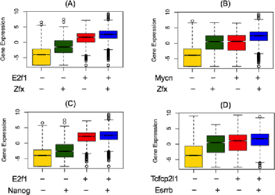
Figure 3: The distribution of gene expression levels given the signs (“$+$” or “$-$”) of TF motif matching scores. (A) E2f1 and Zfx (ranked among top $3$ by both SIRI and COP) show additive effects. (B) Gene expression level is significantly lower when both Mycn (ranked 4 by SIRI and 10 by COP) and Zfx have negative scores. (C) The matching score of Nanog (ranked 14 by SIRI and missed by COP) has an effect on gene expression only when E2f1 also has a negative score. (D) Tcfcp2l1 (ranked 10 by SIRI and 36 by COP) and Esrrb (ranked 8 by SIRI and missed by COP) have nonadditive effects in regulating gene expression.

Zhong et al. (2012) reported that COP selected a total of $42$ predictors, which include $8$ of the $12$ TFASs and $34$ of the $300$ TF motif scores. Here, we used SIRI-AE to re-analyze the mouse ESCs data set and selected $34$ predictors, which include all the $12$ TFASs and $22$ TF motif matching scores. Relative ranks of the $12$ TFASs from SIRI-AE and COP are shown in Table 8. Among the top-$10$ TFs ranked by SIRI-AE, $8$ of them are known ES-cell TFs. SIRI-AE is also able to identify Nanog and Sox that are generally believed to be the master ESC regulators but were missed in the results of COP. The ranked list of 22 other TFs seleted by SIRI is given in Jiang and Liu (2014). A further study of these TFs whose roles in ES cells have not been well understood could help us better understand transcriptional regulatory networks in embryonic stem cells.

In Figure 3, we illustrate combinatorial effects of several identified TFs by plotting the distribution of gene expression levels given the signs of a pair of TF motif matching scores. In Figure 3(A), E2f1 and Zfx (ranked among top $3$ by both SIRI and COP) have additive effects, that is, the combined effect of two TFs is approximately equal to the sum of their individual effects (which can be described by a linear model). The joint effects of TFs in Figure 3(B), (C) and (D) show nonadditive patterns. For example, in Figure 3(B), gene expression levels are significantly lower when both Mycn and Zfx have negative matching scores compared with other scenarios. A similar pattern is observed for Tcfcp2l1 and Esrrb in Figure 3(D). Figure 3(C) shows that the effect of Nanog is only present when E2f1 has a negative matching score. As a result, COP, which is based on linear combinations of TF matching scores, misses Nanog and Esrrb while ranks Mycn and Tcfcp2l1 relatively lower. SIRI is able to identify these TFs by capturing the nonadditive effects.

7 Concluding remarks

We study the problem of variable selection in high dimensions from an inverse modeling perspective. The contributions of the proposed procedure that we named SIRI are twofold. First, it is effective and computationally efficient in selecting relevant variables among a large set of candidates useful for predicting the response, possibly through complex interactions and other forms of nonlinear effects. Combined with independence screening, SIRI can be used to detect complex relationships in ultra-high dimensionality. Second, SIRI does not impose any specific assumption on the relationship between the predictors and the response, and is a powerful tool for variable selections beyond linear models and for detecting variables with unknown form of nonlinear effects. As a trade-off, SIRI imposes a few assumptions on the distribution of the predictors. As demonstrated in our simulation studies, SIRI has competitive performance when the generative model is different from the inverse model assumption. However, we found that SIRI is not very robust against extreme outliers in values of the predictors. Data preprocessing, such as quantile normalization, is advised when extreme outliers are spotted from exploratory analysis. We have implemented the SIRI procedure using programming language R, and the source code can be downloaded from http://www.people.fas.harvard.edu/~junliu/SIRI/ or requested from the authors directly.

We have adopted an ad hoc rule to choose the slicing scheme in SIRI. By allowing adaptive choices of slices based on observed data, we are currently developing a dynamic programming algorithm to find the optimal slicing scheme under a sliced inverse model. Theoretical studies of such an algorithm, however, is more challenging and delicate. Like other stepwise procedures such as linear stepwise regression, SIRI may encounter issues that are typical to stepwise variable selection methods as discussed in Miller (1984). When relevant predictors have weak marginal effects but strong joint effects, iterative sampling procedures such as Gibbs sampling could be more powerful than stepwise procedures like SIRI. This motivates us to further study the problem of variable selection from a full Bayesian perspective.

The main goal of SIRI is to select relevant predictors with nonlinear (including interaction and other second-order) effects on the response without a specific parametric form. Without a specific parametric form, however, it is impossible to precisely define what an “interaction” means. Interestingly, in many scientific problems, scientists often cannot reach an agreement on what analytic form an interaction should take even if they all agree that the interaction exists. As shown in Zhang and Liu (2007), the inverse modeling approach as in naïve Bayes models (as well as in index models), we can finesse the interaction definition problem by stating that the two predictors $X_{1}$ and $X_{2}$ have interactions if and only if their joint distribution conditional on $Y$, that is, $[X_{1},X_{2}|Y]$, cannot be factored into the product of two marginal conditionals, that is, $[X_{1}|Y][X_{2}|Y]$. In order to be computationally efficient, SIRI does not aim to pinpoint exactly which subsets (e.g., pairs, triplets etc.) of variables are interacting sets, but focuses on the overall set of predictors that may influence $Y$. However, a follow-up study on the selected variables can provide further information on which subsets of variables actually form an “interaction clique” in the sense of Zhang and Liu (2007).

Finally, inverse models are not substitutes of, but complements to, forward models. When a specific form is derived from solid scientific arguments, a forward perspective that treats the distribution of predictors as a nuisance can be more powerful in building predictive models. Depending on one’s research questions and objectives, it may be helpful to alternate between the two perspectives in analyzing and interpreting data.

Appendix: Proofs

.1 Proof of Theorem 1 in Section 2.1

Given the set of relevant predictors indexed by $\mathcal{A}$ with size $|\mathcal{A}|$ in model (2.1), we denote $B_{\mathcal{A}}=\operatorname{Cov}(\mathbb{E}(\mathbf{X}_{\mathcal{A}}|\break S(Y)))$, $W_{\mathcal{A}}=\mathbb{E}(\operatorname{Cov}(\mathbf{X}_{\mathcal{A}}|S(Y)))$ and $\Omega_{\mathcal{A}}=B_{\mathcal{A}}+W_{\mathcal{A}}$. The corresponding sample estimates are given by $\widehat{B}_{\mathcal{A}}$, $\widehat{W}_{\mathcal{A}}$ and $\widehat{\Omega}_{\mathcal{A}}=\widehat{B}_{\mathcal{A}}+\widehat{W}_{\mathcal{A}}$. To prove Theorem 1, we will need the following lemma that is proved in Jiang and Liu (2014).

Lemma 1.

Under the same conditions as in Theorem 1, for any set of predictors indexed by $\mathcal{C}$, we let $\widehat{\lambda}_{i}^{\mathcal{C}}$ be the $i$th largest eigenvalue of $\widehat{\Omega}_{\mathcal{C}}^{-1}\widehat{B}_{\mathcal{C}}$ and let $\lambda_{i}^{\mathcal{C}}$ be the $i$th largest eigenvalue of $\Omega_{\mathcal{C}}^{-1}B_{\mathcal{C}}$. Then, for $0<\varepsilon<1$ and $i=1,2,\ldots,q$, there exist positive constants $C_{1}$ and $C_{2}$ such that

$$\operatorname{Pr}\Bigl{(}\max_{\mathcal{C}\subset\{1,2,\ldots,p\}}\bigl{|}\log\bigl{(}1-\widehat{\lambda}_{i}^{\mathcal{C}}\bigr{)}-\log\bigl{(}1-\lambda_{i}^{\mathcal{C}}\bigr{)}\bigr{|}>\varepsilon\Bigr{)}$$

(12)

$$\qquad\leq 2p(p+1)C_{1}\exp{\biggl{(}-C_{2}n\frac{\tau_{\mathrm{min}}^{4}\varepsilon^{2}}{64\tau_{\mathrm{max}}^{2}p^{2}}\biggr{)}},$$

where $\tau_{\mathrm{min}}$ and $\tau_{\mathrm{max}}$ are defined in Condition 1.

Proof of Theorem 1 Let $R_{\mathcal{C}}=\sum_{i=1}^{q}\log(1-\widehat{\lambda}_{i}^{\mathcal{C}})-\sum_{i=1}^{q}\log(1-\lambda_{i}^{\mathcal{C}})$. Then, according to Lemma 1, for $0<\varepsilon<1$, there exist constant $C_{1}$ and $C_{2}$ such that

$$\operatorname{Pr}\Bigl{(}\max_{\mathcal{C}\subset\{1,2,\ldots,p\}}|R_{\mathcal{C}}|>\varepsilon\Bigr{)}\leq 2p(p+1)qC_{1}\exp{\biggl{(}-C_{2}n\frac{\tau_{\mathrm{min}}^{4}\varepsilon^{2}}{64\tau_{\mathrm{max}}^{2}p^{2}q^{2}}\biggr{)}}.$$

Under Condition 2, $p=o(n^{\rho})$ with $2\rho+2\kappa<1$, and for any positive constant $C$,

$$\operatorname{Pr}\Bigl{(}\max_{\mathcal{C}\subset\{1,2,\ldots,p\}}|R_{\mathcal{C}}|>Cn^{-\kappa}\Bigr{)}$$

$$\qquad\leq 2p(p+1)qC_{1}\exp{\biggl{(}-C_{2}n^{1-2\kappa-2\rho}\frac{\tau_{\mathrm{min}}^{4}C^{2}}{64\tau_{\mathrm{max}}^{2}q^{2}}\biggr{)}}\rightarrow 0$$

as $n\rightarrow\infty$. For $j\notin\mathcal{C}$ and $d=|\mathcal{C}|$,

$$\widehat{D}_{j|\mathcal{C}} = -\sum_{i=1}^{q}\log\bigl{(}1-\widehat{\lambda}_{i}^{d+1}\bigr{)}+\sum_{i=1}^{q}\log\bigl{(}1-\widehat{\lambda}_{i}^{d}\bigr{)}$$

$$= -\sum_{i=1}^{q}\log\bigl{(}1-\lambda_{i}^{d+1}\bigr{)}+\sum_{i=1}^{q}\log\bigl{(}1-\lambda_{i}^{d}\bigr{)}-R_{[\mathcal{C}\cup\{j\}]}+R_{\mathcal{C}}$$

$$= \log\biggl{(}1+\frac{\operatorname{Var}(M_{j})-\operatorname{Cov}(M_{j},\mathbf{X}_{\mathcal{C}})[\operatorname{Cov}(\mathbf{X}_{\mathcal{C}})]^{-1}\operatorname{Cov}(M_{j},\mathbf{X}_{\mathcal{C}})^{T}}{\mathbb{E}(V_{j})}\biggr{)}$$

$$-R_{[\mathcal{C}\cup\{j\}]}+R_{\mathcal{C}},$$

where $M_{j}=\mathbb{E}(X_{j}|\mathbf{X}_{\mathcal{C}},S(Y))$, $V_{j}=\operatorname{Var}(X_{j}|\mathbf{X}_{\mathcal{C}},S(Y))$, and $V_{j}$ is a constant that does not depend on $\mathbf{X}_{\mathcal{C}}$ or $S(Y)$ under model (2.1).

When $\mathcal{C}^{c}\cap\mathcal{A}\neq\varnothing$, according to definition of first-order detectable predictors, there exist $\kappa\geq 0$ and $\xi_{0}>0$ such that

$$\max_{j\in\mathcal{C}^{c}\cap\mathcal{A}}\biggl{[}\frac{\operatorname{Var}(M_{j})-\operatorname{Cov}(M_{j},\mathbf{X}_{\mathcal{C}})[\operatorname{Cov}(\mathbf{X}_{\mathcal{C}})]^{-1}\operatorname{Cov}(M_{j},\mathbf{X}_{\mathcal{C}})^{T}}{\mathbb{E}(V_{j})}\biggr{]}\geq\xi_{0}n^{-\kappa}.$$

Then, for sufficiently large $n$, there exists $j\in\mathcal{C}^{c}\cap\mathcal{A}$ such that

$$\log\biggl{(}1+\frac{\operatorname{Var}(M_{j})-\operatorname{Cov}(M_{j},\mathbf{X}_{\mathcal{C}})[\operatorname{Cov}(\mathbf{X}_{\mathcal{C}})]^{-1}\operatorname{Cov}(M_{j},\mathbf{X}_{\mathcal{C}})^{T}}{\mathbb{E}(V_{j})}\biggr{)}\geq\frac{\xi_{1}}{2}n^{-\kappa}$$

and

$$\widehat{D}_{j|\mathcal{C}}\geq\frac{\xi_{1}}{2}n^{-\kappa}-\bigl{(}|R_{[\mathcal{C}\cup\{j\}]}|+|R_{\mathcal{C}}|\bigr{)}.$$

Let $c=\frac{\xi_{0}}{4}$. Since

$$\operatorname{Pr}\biggl{(}\max_{\mathcal{C}\subset\{1,2,\ldots,p\}}|R_{\mathcal{C}}|>\frac{c}{2}n^{-\kappa}\biggr{)}\rightarrow 0,$$

we have

$$\operatorname{Pr}\Bigl{(}\min_{\mathcal{C}\dvtx\mathcal{C}^{c}\cap\mathcal{A}\neq\varnothing}\max_{j\in\mathcal{C}^{c}\cap\mathcal{A}}\widehat{D}_{j|\mathcal{C}}\geq cn^{-\kappa}\Bigr{)}\rightarrow 1,$$

as $n\rightarrow\infty$.

When variable $\mathcal{C}^{c}\cap\mathcal{A}=\varnothing$, for $j\in\mathcal{C}^{c}\subset\mathcal{A}^{c}$, $M_{j}=\mathbb{E}(X_{j}|\mathbf{X}_{\mathcal{C}},S(Y))=\mathbb{E}(X_{j}|\mathbf{X}_{\mathcal{C}})$ is a linear combination of $\mathbf{X}_{\mathcal{C}}$ under model (2.1), and

$$\frac{\operatorname{Var}(M_{j})-\operatorname{Cov}(M_{j},\mathbf{X}_{\mathcal{C}})[\operatorname{Cov}(\mathbf{X}_{\mathcal{C}})]^{-1}\operatorname{Cov}(M_{j},\mathbf{X}_{\mathcal{C}})^{T}}{\mathbb{E}(V_{j})}=0.$$

Thus,

$$\widehat{D}_{j|\mathcal{C}}\leq\bigl{(}|R_{[\mathcal{C}\cup\{j\}]}|+|R_{\mathcal{C}}|\bigr{)}$$

and

$$\operatorname{Pr}\Bigl{(}\max_{\mathcal{C}\dvtx\mathcal{C}^{c}\cap\mathcal{A}=\varnothing}\max_{j\in\mathcal{C}^{c}}\widehat{D}_{j|\mathcal{C}}\geq Cn^{-\kappa}\Bigr{)}\leq\operatorname{Pr}\biggl{(}\max_{\mathcal{C}\subset\{1,2,\ldots,p\}}|R_{\mathcal{C}}|\geq\frac{C}{2}n^{-\kappa}\biggr{)}\rightarrow 0$$

for any positive constant $C$ as $n\rightarrow\infty$.

.2 Proof of Theorem 2 in Section 2.2

Lemma 2.

Under the same condition as in Theorem 2, for $0<\varepsilon<1$, there exist positive constants $C_{1}$ and $C_{2}$ such that

$$\operatorname{Pr}\Bigl{(}\max_{\mathcal{C}\subset\{1,2,\ldots,p\}}\max_{j\in\mathcal{C}^{c}}\bigl{|}\log\widehat{\sigma}_{j|\mathcal{C}}^{2}-\log\sigma_{j|\mathcal{C}}^{2}\bigr{|}>\varepsilon\Bigr{)}\leq\frac{p(p+1)}{2}C_{1}\exp\biggl{(}-C_{2}n\frac{\varepsilon^{2}}{p^{2}L^{2}}\biggr{)}$$

and

$$\operatorname{Pr}\Biggl{(}\max_{\mathcal{C}\subset\{1,2,\ldots,p\}}\max_{j\in\mathcal{C}^{c}}\Biggl{|}\sum_{h=1}^{H}s_{h}\log\bigl{[}\widehat{\sigma}_{j|\mathcal{C}}^{(h)}\bigr{]}^{2}-\sum_{h=1}^{H}s_{h}\log\bigl{[}\sigma_{j|\mathcal{C}}^{(h)}\bigr{]}^{2}\Biggr{|}>\varepsilon\Biggr{)}$$

$$\qquad\leq\frac{Hp(p+1)}{2}C_{1}\exp\biggl{(}-C_{2}n\frac{\varepsilon^{2}}{H^{2}p^{2}L^{2}}\biggr{)},$$

where $L=\frac{4}{\tau_{\mathrm{min}}}(3(\frac{\tau_{\mathrm{max}}}{\tau_{\mathrm{min}}})^{3/2}+1)$, and $\tau_{\mathrm{min}}$ and $\tau_{\mathrm{max}}$ are defined in Condition 1.

Proof of Theorem 2 We denote $R_{j|\mathcal{C}}=\log\widehat{\sigma}_{j|\mathcal{C}}^{2}-\log\sigma_{j|\mathcal{C}}^{2}$ and

$$\widetilde{R}_{j|\mathcal{C}}=\sum_{h=1}^{H}s_{h}\log\bigl{[}\widehat{\sigma}_{j|\mathcal{C}}^{(h)}\bigr{]}^{2}-\sum_{h=1}^{H}s_{h}\log\bigl{[}\sigma_{j|\mathcal{C}}^{(h)}\bigr{]}^{2}.$$

According to Lemma 2, for $0<\varepsilon<1$, there exist $C_{1}$ and $C_{2}$ such that

$$\operatorname{Pr}\Bigl{(}\max_{\mathcal{C}\subset\{1,2,\ldots,p\}}\max_{j\in\mathcal{C}^{c}}|R_{j|\mathcal{C}}|>\varepsilon\Bigr{)}\leq\frac{p(p+1)}{2}C_{1}\exp\biggl{(}-C_{2}n\frac{\varepsilon^{2}}{p^{2}L^{2}}\biggr{)}$$

and

$$\operatorname{Pr}\Bigl{(}\max_{\mathcal{C}\subset\{1,2,\ldots,p\}}\max_{j\in\mathcal{C}^{c}}|\widetilde{R}_{j|\mathcal{C}}|>\varepsilon\Bigr{)}\leq\frac{Hp(p+1)}{2}C_{1}\exp\biggl{(}-C_{2}n\frac{\varepsilon^{2}}{H^{2}p^{2}L^{2}}\biggr{)},$$

where $L=\frac{4}{\tau_{\mathrm{min}}}(3(\frac{\tau_{\mathrm{max}}}{\tau_{\mathrm{min}}})^{3/2}+1)$. Under Condition 2, $p=o(n^{\rho})$ and $2\rho+2\kappa<1$,

$$\operatorname{Pr}\Bigl{(}\max_{\mathcal{C}\subset\{1,2,\ldots,p\}}\max_{j\in\mathcal{C}^{c}}|R_{j|\mathcal{C}}|>Cn^{-\kappa}\Bigr{)}$$

$$\qquad\leq\frac{p(p+1)}{2}C_{1}\exp{\biggl{(}-C_{2}n^{1-2\kappa-2\rho}\frac{C^{2}}{L^{2}}\biggr{)}}\rightarrow 0$$

and

$$\operatorname{Pr}\Bigl{(}\max_{\mathcal{C}\subset\{1,2,\ldots,p\}}\max_{j\in\mathcal{C}^{c}}|\widetilde{R}_{j|\mathcal{C}}|>Cn^{-\kappa}\Bigr{)}$$

$$\qquad\leq\frac{Hp(p+1)}{2}C_{1}\exp{\biggl{(}-C_{2}n^{1-2\kappa-2\rho}\frac{C^{2}}{H^{2}L^{2}}\biggr{)}}\rightarrow 0,$$

for any positive constant $C$ as $n\rightarrow\infty$. We have

$$\widehat{D}^{*}_{j|\mathcal{C}} = \log\widehat{\sigma}_{j|\mathcal{C}}^{2}-\sum_{h=1}^{H}s_{h}\log\bigl{[}\widehat{\sigma}_{j|\mathcal{C}}^{(h)}\bigr{]}^{2}$$

$$= \log\sigma_{j|\mathcal{C}}^{2}-\sum_{h=1}^{H}s_{h}\log\bigl{[}\sigma_{j|\mathcal{C}}^{(h)}\bigr{]}^{2}+R_{j|\mathcal{C}}-\widetilde{R}_{j|\mathcal{C}}$$

$$= \log\biggl{(}1+\frac{\operatorname{Var}(M_{j})-\operatorname{Cov}(M_{j},\mathbf{X}_{\mathcal{C}})[\operatorname{Cov}(\mathbf{X}_{\mathcal{C}})]^{-1}\operatorname{Cov}(M_{j},\mathbf{X}_{\mathcal{C}})^{T}}{\mathbb{E}(V_{j})}\biggr{)}$$

$${}+\log(\mathbb{E}V_{j})-\mathbb{E}\log(V_{j})+R_{j|\mathcal{C}}-\widetilde{R}_{j|\mathcal{C}},$$

where $M_{j}=\mathbb{E}(X_{j}|\mathbf{X}_{\mathcal{C}},S(Y))$ and $V_{j}=\operatorname{Var}(X_{j}|\mathbf{X}_{\mathcal{C}},S(Y))$.

When $\mathcal{C}^{c}\cap\mathcal{A}\neq\varnothing$ and all the relevant predictors indexed by $\mathcal{A}$ are stepwise detectable with constant $\kappa$, then there exists $m\geq 0$ such that $\bigcup_{i=0}^{m-1}\mathcal{T}_{i}\subset\mathcal{C}$ and $\mathcal{C}^{c}\cap\mathcal{T}_{m}\neq\varnothing$. According to Definition 3, there exist $j\in\mathcal{C}^{c}\cap\mathcal{T}_{m}$ and $\xi_{1},\xi_{2}>0$ such that either

$$\frac{\operatorname{Var}(M_{j})-\operatorname{Cov}(M_{j},\mathbf{X}_{\mathcal{C}})[\operatorname{Cov}(\mathbf{X}_{\mathcal{C}})]^{-1}\operatorname{Cov}(M_{j},\mathbf{X}_{\mathcal{C}})^{T}}{\mathbb{E}(V_{j})}\geq\xi_{1}n^{-\kappa},$$

that is, with sufficiently large $n$,

$$\log\biggl{(}1+\frac{\operatorname{Var}(M_{j})-\operatorname{Cov}(M_{j},\mathbf{X}_{\mathcal{C}})[\operatorname{Cov}(\mathbf{X}_{\mathcal{C}})]^{-1}\operatorname{Cov}(M_{j},\mathbf{X}_{\mathcal{C}})^{T}}{\mathbb{E}(V_{j})}\biggr{)}\geq\frac{\xi_{1}}{2}n^{-\kappa}$$

or

$$\log(\mathbb{E}V_{j})-\mathbb{E}\log(V_{j})\geq\xi_{2}n^{-\kappa}.$$

Let $c=\min(\frac{\xi_{1}}{4},\frac{\xi_{2}}{2})$. Therefore,

$$\widehat{D}^{*}_{j|\mathcal{C}} \geq \log\biggl{(}1+\frac{\operatorname{Var}(M_{j})-\operatorname{Cov}(M_{j},\mathbf{X}_{\mathcal{C}})[\operatorname{Cov}(\mathbf{X}_{\mathcal{C}})]^{-1}\operatorname{Cov}(M_{j},\mathbf{X}_{\mathcal{C}})^{T}}{\mathbb{E}(V_{j})}\biggr{)}$$

$${}+\log(\mathbb{E}V_{j})-\mathbb{E}\log(V_{j})-\bigl{(}|R_{j|\mathcal{C}}|+|\widetilde{R}_{j|\mathcal{C}}|\bigr{)}$$

$$\geq 2cn^{-\kappa}-\bigl{(}|R_{j|\mathcal{C}}|+|\widetilde{R}_{j|\mathcal{C}}|\bigr{)}.$$

Since

$$\operatorname{Pr}\biggl{(}\max_{\mathcal{C}\subset\{1,2,\ldots,p\}}\max_{j\in\mathcal{C}^{c}}|R_{j|\mathcal{C}}|>\frac{c}{2}n^{-\kappa}\biggr{)}\rightarrow 0$$

and

$$\operatorname{Pr}\biggl{(}\max_{\mathcal{C}\subset\{1,2,\ldots,p\}}\max_{j\in\mathcal{C}^{c}}|\widetilde{R}_{j|\mathcal{C}}|>\frac{c}{2}n^{-\kappa}\biggr{)}\rightarrow 0,$$

we have

$$\operatorname{Pr}\Bigl{(}\min_{\mathcal{C}\dvtx\mathcal{C}^{c}\cap\mathcal{A}\neq\varnothing}\max_{j\in\mathcal{C}^{c}\cap\mathcal{A}}\widehat{D}^{*}_{j|\mathcal{C}}\geq cn^{-\kappa}\Bigr{)}\rightarrow 1,$$

as $n\rightarrow\infty$.

When $\mathcal{C}^{c}\cap\mathcal{A}=\varnothing$ under model (2.2), for any $j\in\mathcal{C}^{c}$, $M_{j}=\mathbb{E}(X_{j}|\mathbf{X}_{\mathcal{C}},\break S(Y))=\mathbb{E}(X_{j}|\mathbf{X}_{\mathcal{C}})$, which is a linear combination of predictors in $\mathbf{X}_{\mathcal{C}}$, and $V_{j}=\operatorname{Var}(X_{j}|\mathbf{X}_{\mathcal{C}},S(Y))=\operatorname{Var}(X_{j}|\mathbf{X}_{\mathcal{C}})$, which is a constant that does not depend on $\mathbf{X}_{\mathcal{C}}$ or $S(Y)$. Then

$$\frac{\operatorname{Var}(M_{j})-\operatorname{Cov}(M_{j},\mathbf{X}_{\mathcal{C}})[\operatorname{Cov}(\mathbf{X}_{\mathcal{C}})]^{-1}\operatorname{Cov}(M_{j},\mathbf{X}_{\mathcal{C}})^{T}}{\mathbb{E}(V_{j})}=0$$

and

$$\log(\mathbb{E}V_{j})-\mathbb{E}\log(V_{j})=0.$$

Thus,

$$\widehat{D}^{*}_{j|\mathcal{C}}\leq|R_{j|\mathcal{C}}|+|\widetilde{R}_{j|\mathcal{C}}|$$

and

$$\operatorname{Pr}\Bigl{(}\max_{\mathcal{C}\dvtx\mathcal{C}^{c}\cap\mathcal{A}=\varnothing}\max_{j\in\mathcal{C}^{c}}\widehat{D}^{*}_{j|\mathcal{C}}<Cn^{-\kappa}\Bigr{)}\rightarrow 1,$$

for any positive constant $C$ as $n\rightarrow\infty$.

References

- Bien, Taylor and Tibshirani (2013) {barticle}[mr] \bauthor\bsnmBien, \bfnmJacob\binitsJ., \bauthor\bsnmTaylor, \bfnmJonathan\binitsJ. and \bauthor\bsnmTibshirani, \bfnmRobert\binitsR. (\byear2013). \btitleA LASSO for hierarchical interactions. \bjournalAnn. Statist. \bvolume41 \bpages1111–1141. \biddoi=10.1214/13-AOS1096, issn=0090-5364, mr=3113805 \bptokimsref\endbibitem
- Chen and Li (1998) {barticle}[mr] \bauthor\bsnmChen, \bfnmChun-Houh\binitsC.-H. and \bauthor\bsnmLi, \bfnmKer-Chau\binitsK.-C. (\byear1998). \btitleCan SIR be as popular as multiple linear regression? \bjournalStatist. Sinica \bvolume8 \bpages289–316. \bidissn=1017-0405, mr=1624402 \bptokimsref\endbibitem
- Chen et al. (2008) {barticle}[author] \bauthor\bsnmChen, \bfnmXi\binitsX., \bauthor\bsnmXu, \bfnmHan\binitsH., \bauthor\bsnmYuan, \bfnmPing\binitsP., \bauthor\bsnmFang, \bfnmFang\binitsF., \bauthor\bsnmHuss, \bfnmMikael\binitsM., \bauthor\bsnmVega, \bfnmVinsensius B.\binitsV. B., \bauthor\bsnmWong, \bfnmEleanor\binitsE., \bauthor\bsnmOrlov, \bfnmYuriy L.\binitsY. L., \bauthor\bsnmZhang, \bfnmWeiwei\binitsW., \bauthor\bsnmJiang, \bfnmJianming\binitsJ. \betalet al. (\byear2008). \btitleIntegration of external signaling pathways with the core transcriptional network in embryonic stem cells. \bjournalCell \bvolume133 \bpages1106–1117. \bptokimsref\endbibitem
- Cloonan et al. (2008) {barticle}[author] \bauthor\bsnmCloonan, \bfnmNicole\binitsN., \bauthor\bsnmForrest, \bfnmAlistair RR\binitsA. R., \bauthor\bsnmKolle, \bfnmGabriel\binitsG., \bauthor\bsnmGardiner, \bfnmBrooke BA\binitsB. B., \bauthor\bsnmFaulkner, \bfnmGeoffrey J.\binitsG. J., \bauthor\bsnmBrown, \bfnmMellissa K.\binitsM. K., \bauthor\bsnmTaylor, \bfnmDarrin F.\binitsD. F., \bauthor\bsnmSteptoe, \bfnmAnita L.\binitsA. L., \bauthor\bsnmWani, \bfnmShivangi\binitsS., \bauthor\bsnmBethel, \bfnmGraeme\binitsG. \betalet al. (\byear2008). \btitleStem cell transcriptome profiling via massive-scale mRNA sequencing. \bjournalNature Methods \bvolume5 \bpages613–619. \bptokimsref\endbibitem
- Cook (2004) {barticle}[mr] \bauthor\bsnmCook, \bfnmR. Dennis\binitsR. D. (\byear2004). \btitleTesting predictor contributions in sufficient dimension reduction. \bjournalAnn. Statist. \bvolume32 \bpages1062–1092. \biddoi=10.1214/009053604000000292, issn=0090-5364, mr=2065198 \bptokimsref\endbibitem
- Cook (2007) {barticle}[mr] \bauthor\bsnmCook, \bfnmR. Dennis\binitsR. D. (\byear2007). \btitleFisher lecture: Dimension reduction in regression. \bjournalStatist. Sci. \bvolume22 \bpages1–26. \biddoi=10.1214/088342306000000682, issn=0883-4237, mr=2408655 \bptokimsref\endbibitem
- Efron et al. (2004) {barticle}[mr] \bauthor\bsnmEfron, \bfnmBradley\binitsB., \bauthor\bsnmHastie, \bfnmTrevor\binitsT., \bauthor\bsnmJohnstone, \bfnmIain\binitsI. and \bauthor\bsnmTibshirani, \bfnmRobert\binitsR. (\byear2004). \btitleLeast angle regression. \bjournalAnn. Statist. \bvolume32 \bpages407–499. \biddoi=10.1214/009053604000000067, issn=0090-5364, mr=2060166 \bptokimsref\endbibitem
- Fan and Li (2001) {barticle}[mr] \bauthor\bsnmFan, \bfnmJianqing\binitsJ. and \bauthor\bsnmLi, \bfnmRunze\binitsR. (\byear2001). \btitleVariable selection via nonconcave penalized likelihood and its oracle properties. \bjournalJ. Amer. Statist. Assoc. \bvolume96 \bpages1348–1360. \biddoi=10.1198/016214501753382273, issn=0162-1459, mr=1946581 \bptokimsref\endbibitem
- Fan and Lv (2008) {barticle}[mr] \bauthor\bsnmFan, \bfnmJianqing\binitsJ. and \bauthor\bsnmLv, \bfnmJinchi\binitsJ. (\byear2008). \btitleSure independence screening for ultrahigh dimensional feature space. \bjournalJ. R. Stat. Soc. Ser. B Stat. Methodol. \bvolume70 \bpages849–911. \biddoi=10.1111/j.1467-9868.2008.00674.x, issn=1369-7412, mr=2530322 \bptokimsref\endbibitem
- Friedman et al. (2007) {barticle}[mr] \bauthor\bsnmFriedman, \bfnmJerome\binitsJ., \bauthor\bsnmHastie, \bfnmTrevor\binitsT., \bauthor\bsnmHöfling, \bfnmHolger\binitsH. and \bauthor\bsnmTibshirani, \bfnmRobert\binitsR. (\byear2007). \btitlePathwise coordinate optimization. \bjournalAnn. Appl. Stat. \bvolume1 \bpages302–332. \biddoi=10.1214/07-AOAS131, issn=1932-6157, mr=2415737 \bptokimsref\endbibitem
- Golub et al. (1999) {barticle}[author] \bauthor\bsnmGolub, \bfnmTodd R.\binitsT. R., \bauthor\bsnmSlonim, \bfnmDonna K.\binitsD. K., \bauthor\bsnmTamayo, \bfnmPablo\binitsP., \bauthor\bsnmHuard, \bfnmChristine\binitsC., \bauthor\bsnmGaasenbeek, \bfnmMichelle\binitsM., \bauthor\bsnmMesirov, \bfnmJill P.\binitsJ. P., \bauthor\bsnmColler, \bfnmHilary\binitsH., \bauthor\bsnmLoh, \bfnmMignon L.\binitsM. L., \bauthor\bsnmDowning, \bfnmJames R.\binitsJ. R., \bauthor\bsnmCaligiuri, \bfnmMark A.\binitsM. A. \betalet al. (\byear1999). \btitleMolecular classification of cancer: Class discovery and class prediction by gene expression monitoring. \bjournalScience \bvolume286 \bpages531–537. \bptokimsref\endbibitem
- Jiang and Liu (2014) {bmisc}[author] \bauthor\bsnmJiang, \binitsB. and \bauthor\bsnmLiu, \binitsJ. S. (\byear2014). \bhowpublishedSupplement to “Variable selection for general index models via sliced inverse regression.” DOI:\doiurl10.1214/14-AOS1233SUPP. \bptokimsref \endbibitem
- Li (1991) {barticle}[mr] \bauthor\bsnmLi, \bfnmKer-Chau\binitsK.-C. (\byear1991). \btitleSliced inverse regression for dimension reduction. \bjournalJ. Amer. Statist. Assoc. \bvolume86 \bpages316–342. \bidissn=0162-1459, mr=1137117 \bptokimsref\endbibitem
- Li (2007) {barticle}[mr] \bauthor\bsnmLi, \bfnmLexin\binitsL. (\byear2007). \btitleSparse sufficient dimension reduction. \bjournalBiometrika \bvolume94 \bpages603–613. \biddoi=10.1093/biomet/asm044, issn=0006-3444, mr=2410011 \bptokimsref\endbibitem
- Li, Cook and Nachtsheim (2005) {barticle}[mr] \bauthor\bsnmLi, \bfnmLexin\binitsL., \bauthor\bsnmCook, \bfnmR. Dennis\binitsR. D. and \bauthor\bsnmNachtsheim, \bfnmChristopher J.\binitsC. J. (\byear2005). \btitleModel-free variable selection. \bjournalJ. R. Stat. Soc. Ser. B Stat. Methodol. \bvolume67 \bpages285–299. \biddoi=10.1111/j.1467-9868.2005.00502.x, issn=1369-7412, mr=2137326 \bptokimsref\endbibitem
- Li, Zhong and Zhu (2012) {barticle}[mr] \bauthor\bsnmLi, \bfnmRunze\binitsR., \bauthor\bsnmZhong, \bfnmWei\binitsW. and \bauthor\bsnmZhu, \bfnmLiping\binitsL. (\byear2012). \btitleFeature screening via distance correlation learning. \bjournalJ. Amer. Statist. Assoc. \bvolume107 \bpages1129–1139. \biddoi=10.1080/01621459.2012.695654, issn=0162-1459, mr=3010900 \bptokimsref\endbibitem
- Miller (1984) {barticle}[mr] \bauthor\bsnmMiller, \bfnmAlan J.\binitsA. J. (\byear1984). \btitleSelection of subsets of regression variables. \bjournalJ. Roy. Statist. Soc. Ser. A \bvolume147 \bpages389–425. \biddoi=10.2307/2981576, issn=0035-9238, mr=0769997 \bptokimsref\endbibitem
- Murphy, Dean and Raftery (2010) {barticle}[mr] \bauthor\bsnmMurphy, \bfnmThomas Brendan\binitsT. B., \bauthor\bsnmDean, \bfnmNema\binitsN. and \bauthor\bsnmRaftery, \bfnmAdrian E.\binitsA. E. (\byear2010). \btitleVariable selection and updating in model-based discriminant analysis for high dimensional data with food authenticity applications. \bjournalAnn. Appl. Stat. \bvolume4 \bpages396–421. \biddoi=10.1214/09-AOAS279, issn=1932-6157, mr=2758177 \bptokimsref\endbibitem
- Ouyang, Zhou and Wong (2009) {barticle}[pbm] \bauthor\bsnmOuyang, \bfnmZhengqing\binitsZ., \bauthor\bsnmZhou, \bfnmQing\binitsQ. and \bauthor\bsnmWong, \bfnmWing Hung\binitsW. H. (\byear2009). \btitleChIP-Seq of transcription factors predicts absolute and differential gene expression in embryonic stem cells. \bjournalProc. Natl. Acad. Sci. USA \bvolume106 \bpages21521–21526. \biddoi=10.1073/pnas.0904863106, issn=1091-6490, pii=0904863106, pmcid=2789751, pmid=19995984 \bptokimsref\endbibitem
- Ravikumar et al. (2009) {barticle}[mr] \bauthor\bsnmRavikumar, \bfnmPradeep\binitsP., \bauthor\bsnmLafferty, \bfnmJohn\binitsJ., \bauthor\bsnmLiu, \bfnmHan\binitsH. and \bauthor\bsnmWasserman, \bfnmLarry\binitsL. (\byear2009). \btitleSparse additive models. \bjournalJ. R. Stat. Soc. Ser. B Stat. Methodol. \bvolume71 \bpages1009–1030. \biddoi=10.1111/j.1467-9868.2009.00718.x, issn=1369-7412, mr=2750255 \bptokimsref\endbibitem
- Simon and Tibshirani (2012) {bmisc}[author] \bauthor\bsnmSimon, \bfnmNoah\binitsN. and \bauthor\bsnmTibshirani, \bfnmRobert\binitsR. (\byear2012). \bhowpublishedA permutation approach to testing interactions in many dimensions. Preprint. Available at \arxivurlarXiv:1206.6519. \bptokimsref\endbibitem
- Szretter and Yohai (2009) {barticle}[mr] \bauthor\bsnmSzretter, \bfnmMaria Eugenia\binitsM. E. and \bauthor\bsnmYohai, \bfnmVíctor Jaime\binitsV. J. (\byear2009). \btitleThe sliced inverse regression algorithm as a maximum likelihood procedure. \bjournalJ. Statist. Plann. Inference \bvolume139 \bpages3570–3578. \biddoi=10.1016/j.jspi.2009.04.008, issn=0378-3758, mr=2549105 \bptokimsref\endbibitem
- Tibshirani (1996) {barticle}[mr] \bauthor\bsnmTibshirani, \bfnmRobert\binitsR. (\byear1996). \btitleRegression shrinkage and selection via the lasso. \bjournalJ. R. Stat. Soc. Ser. B Stat. Methodol. \bvolume58 \bpages267–288. \bidissn=0035-9246, mr=1379242 \bptokimsref\endbibitem
- Tibshirani et al. (2002) {barticle}[pbm] \bauthor\bsnmTibshirani, \bfnmRobert\binitsR., \bauthor\bsnmHastie, \bfnmTrevor\binitsT., \bauthor\bsnmNarasimhan, \bfnmBalasubramanian\binitsB. and \bauthor\bsnmChu, \bfnmGilbert\binitsG. (\byear2002). \btitleDiagnosis of multiple cancer types by shrunken centroids of gene expression. \bjournalProc. Natl. Acad. Sci. USA \bvolume99 \bpages6567–6572. \biddoi=10.1073/pnas.082099299, issn=0027-8424, pii=99/10/6567, pmcid=124443, pmid=12011421 \bptokimsref\endbibitem
- Zhang and Liu (2007) {barticle}[pbm] \bauthor\bsnmZhang, \bfnmYu\binitsY. and \bauthor\bsnmLiu, \bfnmJun S.\binitsJ. S. (\byear2007). \btitleBayesian inference of epistatic interactions in case–control studies. \bjournalNat. Genet. \bvolume39 \bpages1167–1173. \biddoi=10.1038/ng2110, issn=1061-4036, pii=ng2110, pmid=17721534 \bptokimsref\endbibitem
- Zhong et al. (2005) {barticle}[pbm] \bauthor\bsnmZhong, \bfnmWenxuan\binitsW., \bauthor\bsnmZeng, \bfnmPeng\binitsP., \bauthor\bsnmMa, \bfnmPing\binitsP., \bauthor\bsnmLiu, \bfnmJun S.\binitsJ. S. and \bauthor\bsnmZhu, \bfnmYu\binitsY. (\byear2005). \btitleRSIR: Regularized sliced inverse regression for motif discovery. \bjournalBioinformatics \bvolume21 \bpages4169–4175. \biddoi=10.1093/bioinformatics/bti680, issn=1367-4803, pii=bti680, pmid=16166098 \bptokimsref\endbibitem
- Zhong et al. (2012) {barticle}[mr] \bauthor\bsnmZhong, \bfnmWenxuan\binitsW., \bauthor\bsnmZhang, \bfnmTingting\binitsT., \bauthor\bsnmZhu, \bfnmYu\binitsY. and \bauthor\bsnmLiu, \bfnmJun S.\binitsJ. S. (\byear2012). \btitleCorrelation pursuit: Forward stepwise variable selection for index models. \bjournalJ. R. Stat. Soc. Ser. B Stat. Methodol. \bvolume74 \bpages849–870. \biddoi=10.1111/j.1467-9868.2011.01026.x, issn=1369-7412, mr=2988909 \bptokimsref\endbibitem
- Zou (2006) {barticle}[mr] \bauthor\bsnmZou, \bfnmHui\binitsH. (\byear2006). \btitleThe adaptive lasso and its oracle properties. \bjournalJ. Amer. Statist. Assoc. \bvolume101 \bpages1418–1429. \biddoi=10.1198/016214506000000735, issn=0162-1459, mr=2279469 \bptokimsref\endbibitem