Search for Alfvén waves in a bright network element observed in H$\alpha$

Abstract

Alfvén waves are considered as potential transporters of energy heating the solar corona. We seek spectroscopic signatures of the Alfvén waves in the chromosphere occupied by a bright network element, investigating temporal variations of the spectral width, intensity, Dopplershift, and the asymmetry of the core of the H$\alpha$ spectral line observed by the tunable Lyot filter installed on the Dutch Open Telescope. The spectral characteristics are derived through the fitting of five intensity samples, separated from each other by 0.35 Å, by a $4^{\rm th}$-order polynomial. The bright network element displays the most pronounced variations of the Dopplershift varying from 0 to 4 km s^-1 about the average of 1.5 km s^-1. This fact implies a persistent redshift of the H$\alpha$ core with a redward asymmetry of about 0.5 km s^-1, suggesting an inverse-C bisector. The variations of the core intensity up to $\pm 10$ % and the core width up to $\pm 5$ % about the respective averages are much less pronounced, but still detectable. The core intensity variations lag behind the Dopplershift variations about 2.1 min. The H$\alpha$ core width tends to correlate with the Dopplershift and anticorrelate with the asymmetry, suggesting that more redshifted H$\alpha$ profiles are wider and the broadening of the H$\alpha$ core is accompanied with a change of the core asymmetry from redward to blueward. We also found a striking anticorrelation between the core asymmetry and the Dopplershift, suggesting a change of the core asymmetry from redward to blueward with an increasing redshift of the H$\alpha$ core. The data and the applied analysis do not show meaningful tracks of Alfvén waves in the selected network element.

1 Introduction

Alfvén waves have been invoked as one of possible mechanisms heating the solar corona (Alfvén, 1947; Osterbrock, 1961). These magnetic transporters of convective energy are capable of penetrating through the solar atmosphere without being reflected and refracted. Since Alfvén waves are incompressible, their propagation through the atmosphere is not associated with density changes seen as periodic variations of intensities and line-of-sight velocities (Erdélyi & Fedun, 2007; Mathioudakis et al., 2012). Observation of a slanted magnetic fluxtube could reveal Alfvén waves as periodic variations of nonthermal broadening of a spectral line. This approach was employed in the study by Jess et al. (2009) who found periodic oscillations of nonthermal broadening of the H$\alpha$ spectral line seen over a cluster of bright points associated with a distinct upflow without significant periodic variations of intensities and line-of-sight velocities. They interpret this as a manifestation of Alfvén waves in the solar atmosphere. However, there is some ambiguity whether they deal with spectral or integrated intensities.

Motivated by the results of Jess et al. (2009), we search for signatures of Alfvén waves in a bright network element occupied by a cluster of G-band bright points. We investigate spectral characteristics of the H$\alpha$ spectral line, focusing on temporal variations of the line core width, intensity, Dopplershift, and the asymmetry derived by a $4^{\rm th}$-order-polynomial fitting of a coarse five-point sampling of the H$\alpha$ profile. Since we employ the correcting method and results of Koza et al. (2013), and frequently refer to it as Paper I hereafter, we invite the reader to have it handy.

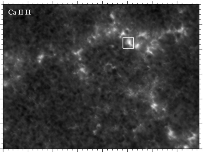
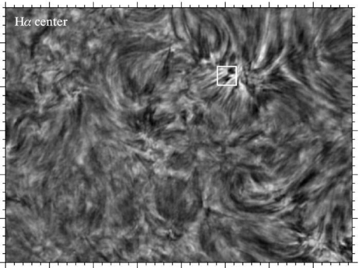
Figure 1: Images of the quiet-Sun network recorded by DOT on 19 October 2005. Top: the temporal mean of the Ca II H image sequence over its 71-min duration. Bottom: the H$\alpha$ image taken at 10:36:21 UT in the line center at the moment of the best seeing occurred in the $41^{\rm st}$ min after the start of the observation at 09:55:20 UT. The square defines the network element selected for this study and displayed in detail in Figs. 4–7. Field of view: 79 $\times$ 58 arcsec². Tickmark spacing: 2 arcsec.

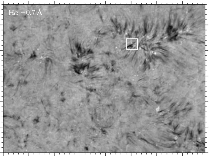
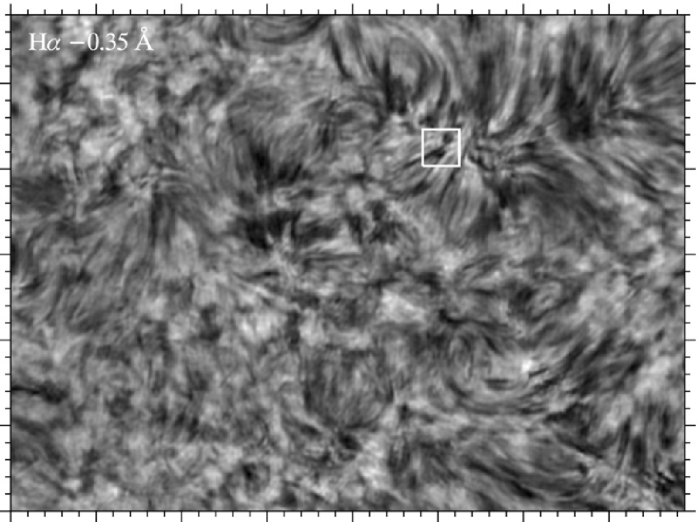
Figure 2: DOT H$\alpha$ images at $\Delta\lambda=-0.7$ Å (top) and $-0.35$ Å (bottom) from the line center corresponding to the H$\alpha$ line-center image in Fig. 1.

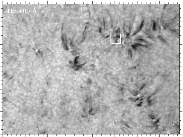
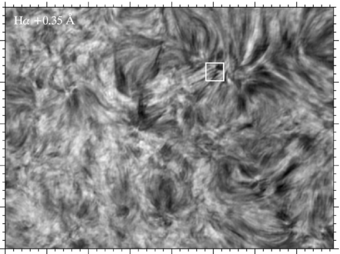
Figure 3: DOT H$\alpha$ images at $\Delta\lambda=+0.7$ Å (top) and +0.35 Å (bottom) from the line center corresponding to the H$\alpha$ images in Figs. 1 and 2.

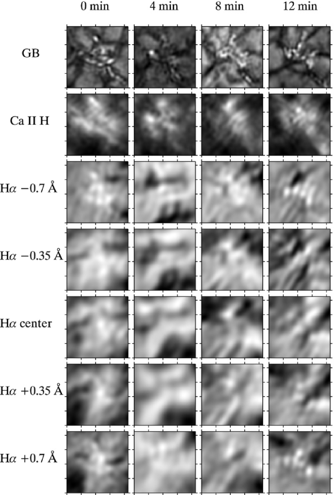
Figure 4: Temporal evolution of the selected network element seen simultaneously in the DOT G-band, Ca II H, and H$\alpha$ images taken at five wavelength settings of the H$\alpha$ Lyot filter. The time 0 min corresponds to the moment of the start of the observation at 09:55:20 UT. Field of view: 4.3 $\times$ 4.3 arcsec². Tickmark spacing: 1 arcsec.

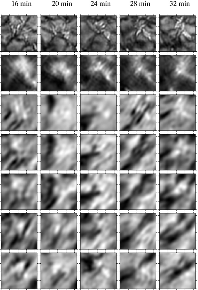
Figure 5: The same as in Fig. 4.

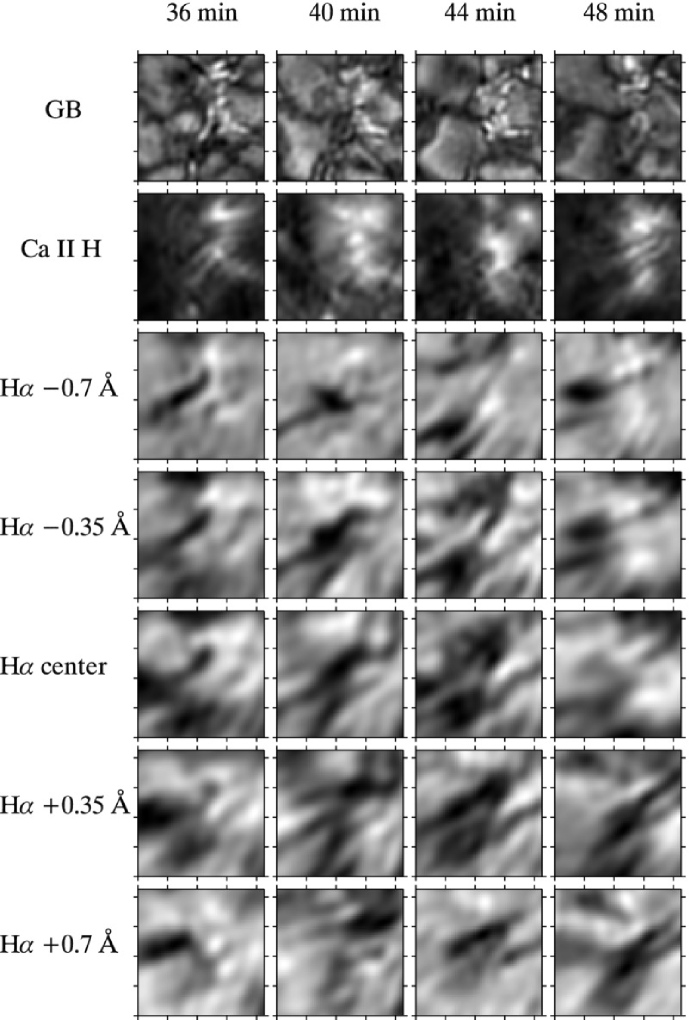
Figure 6: The same as in Fig. 4.

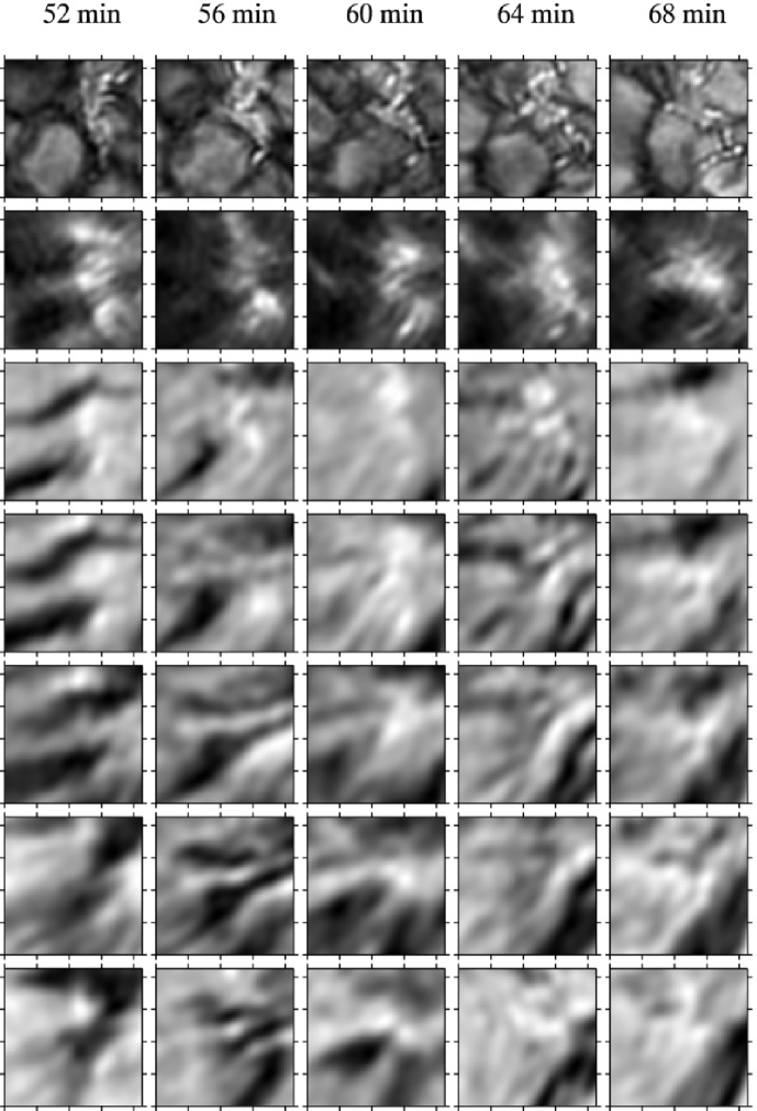
Figure 7: The same as in Fig. 4.

2 Observations

We use sequences of H$\alpha$ images of a very quiet area near the disk center ($\mu=0.91$) recorded by the Dutch Open Telescope (DOT) on 19 October 2005 from 09:55:20 UT to 11:05:47 UT by the tunable Lyot filter with a FWHM passband of 0.25 Å (Gaizauskas, 1976; Bettonvil et al., 2006). The sequence consists of scans taken in five wavelengths across the H$\alpha$ line profile: line center, $\pm 0.35$ Å and $\pm 0.7$ Å, followed by a single image in the line center. The zero wavelength of the filtergrams is centered on the minimum of an average profile taken before the observations over the field of view. A time step between the five-wavelength scans of the H$\alpha$ line profile and line center images is 30 s. Since the images at two subsequent wavelengths are separated by the 4-to-5-s intervals, one full 5-point scan of the H$\alpha$ profile took about 20-25 s. Within this interval no major changes of chromospheric scenery are assumed. The scans were taken in 20-frame bursts per particular wavelength setting and then speckle-reconstructed applying a Keller - von der Lühe two-channel reconstruction (Keller & von der Lühe, 1992). The line center images were obtained in 100-frame bursts restored by a full single-channel speckle reconstruction. In this study, we employ 71 H$\alpha$ scans at a regular 60-s cadence taken between 09:55:20 UT and 11:05:22 UT. The seeing was only fair, with the Fried parameter $r_{0}$ slightly increasing from about 7.5 at the beginning to 9 on average at the end of the observation. As a context data, we also use the sequences of 142 G-band and Ca II H images taken synchronously with the H$\alpha$ images at a regular 30-s cadence. The temporal mean of the Ca II H images and examples of the H$\alpha$ images taken during the period of the best seeing are shown in Figs. 1–3. The size of the Ca II H and H$\alpha$ images is $1112\times 818$ px², with the angular size of pixel of 0.071 arcsec. Details on the DOT, its tomographic multiwavelength imaging, speckle reconstruction, and standard reduction procedures are given in Hammerschlag & Bettonvil (1998) and Rutten et al. (2004).

The target area encompasses a full supergranular cell surrounded by a prominent network as seen in the temporal mean of the Ca II H sequence in Fig. 1. Visual comparison of both panels in Fig. 1 indicates that the brightest network elements coincide with roots of long chromospheric fibrils. These dominate H$\alpha$ scene and emanate out from the network elements outlining the structure of magnetic field at chromospheric levels. DOT H$\alpha$ scans render a tomographic view of the solar atmosphere from the photosphere (Figs. 2 and 3: $\pm 0.7$ Å) up to the chromosphere sampled by the images in the line center and $\pm 0.35$ Å off (Kontogiannis et al., 2010). In the H$\alpha$ $+0.7$ Å image (Fig. 3, top), we can clearly see granulation which is missing in the H$\alpha$ $-0.7$ Å image (Fig. 2, top) due to Doppler cancellation. Both images display dark elongated streaks which are highly-dopplershifted parts of fibrils seen better in the line center and $\pm 0.35$ Å images. Doppler cancellation enhances the visibility of magnetic elements seen as bright points in the H$\alpha$ $-0.7$ Å image (Fig. 2, top), studied in detail in Leenaarts et al. (2006). The square defines the network element selected for this study. The size of the square is $61\times 61$ px², corresponding to $4.3\times 4.3$ arcsec².

Figs. 4–7 show enlargements of the square providing a multispectral tomographic view on evolution of the selected network element unfolded in time with a 4-min timestep from the lower photosphere (G band) up to the chromosphere (H$\alpha$ line center). The G-band cutouts show a cluster of bright points constituting the network element. The selected area also involves two large granules, with maximum diameters larger than 2 arcsec, occurring in the lower half from 16 to 28 min (Fig. 5) and from 44 to 68 min (Figs. 6 and 7). The Ca II H cutouts show brightenings whose overall morphology is often very similar to that of the cluster of the G-band bright points. But the former are strongly diffuse because of resonance scattering within the solar atmosphere and through expansion of idealized magnetostatic fluxtubes with height (Leenaarts et al., 2006). The H$\alpha$ outer wing cutouts ($\pm 0.7$ Å) mix photospheric and chromospheric features because of a double-peak contribution function at H$\alpha$ wings (Schoolman, 1972; Leenaarts et al., 2006, 2012). Striking, almost one-to-one correspondence between the G-band bright points and the blue wing bright points seen in $-0.7$ Å (compare the G-band and H$\alpha$ $-0.7$ Å cutouts, e.g., at 0, 12, 32, 60, and 64 min) was explained in Leenaarts et al. (2006). The line center and $\pm 0.35$ Å cutouts bear still signatures of a network brightening, but modulated much with a fast-changing blanket of the dark fibrils occurring higher up.

3 Method, spectral characteristics, and their corrections

The coarse five-point sampling enables us to construct $1112\times 818\times 71$ instantaneous proxy profiles of the H$\alpha$ spectral line at each pixel. We fit the five-wavelength samples of the proxy profiles by a $4^{\rm th}$-order polynomial to derive the four basic profile measurements: the core intensity $I_{\rm C}$, the core velocity $v_{\rm C}$, the core width FW, and the bisector velocity $v_{\rm BI}$. The values of $I_{\rm C}$ and $v_{\rm C}$ represent the fit minimum and its Dopplershift, respectively. The core width is the wavelength separation of the two fit flanks at half of the intensity range between the fit minimum and the average of the endpoint intensities at $\pm 0.7$ Å. The core width is computed at the average intensity $I_{\rm FW}$ employing the reference intensity $I_{\rm RF1}$ defined by equations (3) and (4) in Paper I. Finally, the bisector velocity is the velocity equivalent of the wavelength separation between the midpoint of the fit at the average intensity $I_{\rm FW}$ and the fit minimum. A more detailed definition of the spectral characteristics is given in Paper I. In case of a large Dopplershift, when the average intensity is larger than the minimum of endpoint intensities, i.e., $I_{\rm FW}>{\rm min}(I_{\rm-0.7},I_{\rm+0.7})$, the fits are extrapolated beyond the range $\pm 0.7$ Å using the polynomial coefficients and the extrapolated fits are used for determining the spectral characteristics. In very rare cases of a polynomial undulation, with local maxima lower than the average intensity $I_{\rm FW}$, the algorithm switches to a parabolic fit of the five-point proxy profile to determine FW, while $I_{\rm C}$ and $v_{\rm C}$ are always from the $4^{\rm th}$-order-polynomial fit and $v_{\rm BI}$ is undefined. The extrapolation (Fig. 8) was invoked just in 0.024 % and the parabolic fit in $5\times 10^{-4}$ % out of all pixels. The intensities shown in Figs. 8 and 9 were normalized with respect to the mean intensities resulting from spatio-temporal averaging of the respective image cubes. The five mean intensities were converted to the atlas intensity scale convolving the H$\alpha$ atlas profile with the transmission profile of the DOT H$\alpha$ filter (Paper I, equation (1)). Therefore, the integrated intensities in Figs. 8 and 9 are in the wavelength unit.

The five intensity samples have an instrumental wavelength scale ranging from $-0.7$ to 0.7 Å. The wavelengths of particular core fit minima $\lambda_{\rm C}$ are measured with respect to this instrumental wavelength scale with milliångström resolution and then converted to the core velocity as: $v_{\rm C}=c(\lambda_{\rm C}-\lambda_{\rm R})/\lambda_{0}$ , where $c$ is the speed of light, $\lambda_{0}$ is the central wavelength of the H$\alpha$ line 6562.8 Å, and the reference wavelength $\lambda_{\rm R}$ is the spatio-temporal average of all $1112\times 818\times 71$ wavelengths of fit minima $\lambda_{\rm C}$ over all pixels within the field of view, making no distinction between network and internetwork pixels. The reference wavelength $\lambda_{\rm R}$ is about $-18$ mÅ. An adopted sign convention indicates a redshift of the line core fit for positive Dopplershift and $v_{\rm C}$. The bisector velocity $v_{\rm BI}$ quantifies an asymmetry of the line core fit with respect to its minimum. The sign convention adopted in Paper I suggests positive $v_{\rm BI}$ for a line core fit with a redward asymmetry.

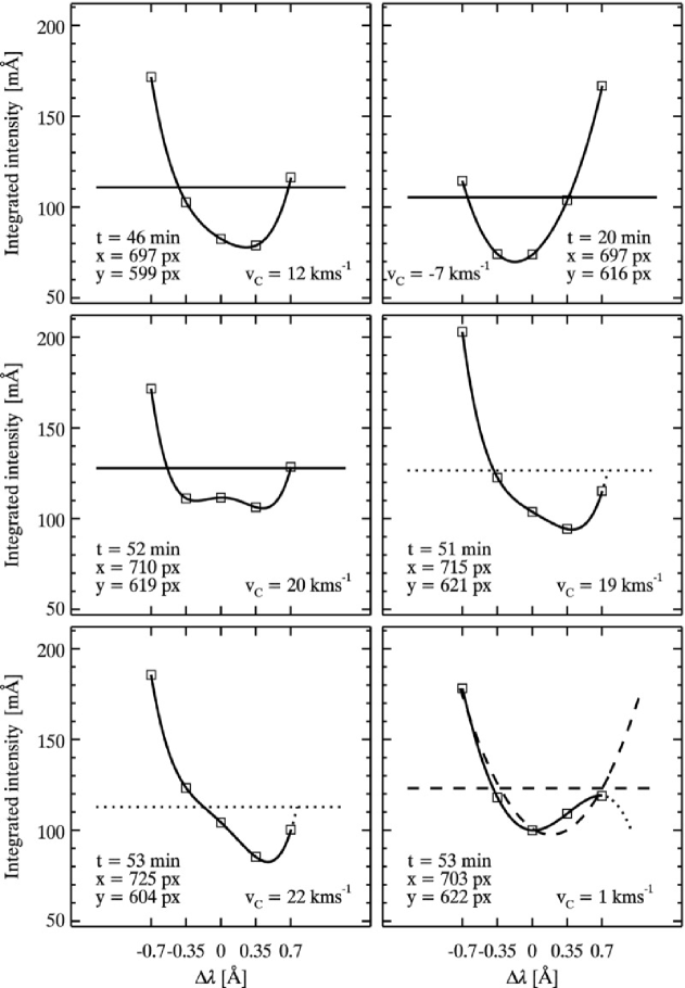
Figure 8: Examples of observed intensities (squares), their $4^{\rm th}$-order-polynomial (solid), extrapolated (dotted), and parabolic (dashed) fits taken from various locations $x,y$ over the selected network element at the indicated time $t$. The horizontal lines indicate the average intensity defining the fit width and the bisector velocity. Their solid, dotted, and dashed linestyles correspond to the $4^{\rm th}$-order-polynomial, extrapolated, and parabolic fits, respectively, used in determination of the fit width and the bisector velocity. The coordinates $x,y$ refer to the lower left corners of images. The selected samples do not represent majority, but rather rare cases with a high core velocity $v_{\rm C}$ and highly asymmetric profiles (the middle and bottom panels).

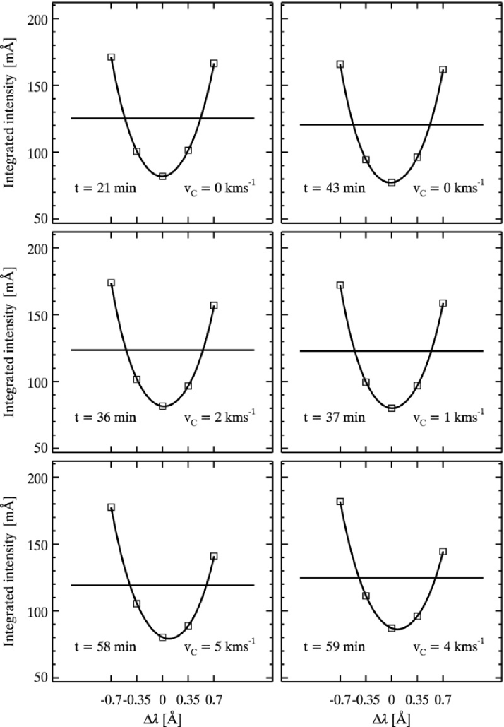
Figure 9: Examples of observed intensities (squares) averaged over the selected network element (Figs. 4–7) and their $4^{\rm th}$-order-polynomial fits (solid) at the given time $t$. The horizontal lines indicate the average intensity defining the fit width and the bisector velocity. The samples illustrate the fits with small (top), medium (middle), and high (bottom) redshift with the core velocity $v_{\rm C}$.

To eliminate the modulation of the spectral characteristics induced by the fast-changing blanket of dark fibrils, we construct 71 proxy H$\alpha$ profiles by spatial averaging of intensities within the selected network element (Figs. 4–7) at each wavelength. Fig. 9 shows examples of these spatially averaged intensities, their polynomial fits, average intensities, and core velocities. Spectral characteristics of these spatially averaged intensities are determined solely from their $4^{\rm th}$-order-polynomial non-extrapolated fits. To asses an influence of the averaging on the final results, we compare them with the instantaneous characteristics obtained by the spatial averaging of FW, $I_{\rm C}$, $v_{\rm C}$, and $v_{\rm BI}$ within the selected area (Figs. 4–7). Both, the instantaneous spectral characteristics inferred per pixel and also from the spatially averaged intensities are corrected for the deviations estimated in Paper I comparing the measurements of FW, $I_{\rm C}$, $v_{\rm C}$, and $v_{\rm BI}$ performed at the dopplershifted H$\alpha$ atlas profile convolved with the filter transmission with their reference values. Then the corrected core velocity $v_{\rm C}$ is the solution of the equation $f(v_{\rm C})+v_{\rm C}-\nu=0$ , where $f(v_{\rm C})$ is the absolute deviation $\Delta v$ and $\nu$ is the measured core velocity. The corrected FW results from the equation $FW=fw-\Delta FW(v_{\rm C})$ , where $fw$ is the measured fit width and $\Delta FW(v_{\rm C})$ is the absolute deviation $\Delta FW$, but interpolated on the corrected core velocity $v_{\rm C}$. The corrected $v_{\rm BI}$ is computed in the same way. Due to different intensity scales, the corrected $I_{\rm C}$ results from the equation $I_{\rm C}=i/(1+\Delta I_{\rm r}(v_{\rm C})/100)$ , where $i$ is the measured core intensity and $\Delta I_{\rm r}(v_{\rm C})$ is the relative deviation $\Delta I_{\rm r}$, but interpolated on the corrected core velocity $v_{\rm C}$.

4 Noise, data uncertainties, and references

Reliability of results inferred by fitting depends critically on the noise presented in the data and various intrinsic uncertainties. Therefore, in this section we give a brief account of uncertainties of the fitted intensities and the reference wavelength defining the core velocity.

We estimated the upper limit of the noise level $1\sigma_{\rm NOISE}$ presented in the H$\alpha$ filtergrams from $1\sigma$ of the temporal variations of the intensity at each pixel assuming that $1\sigma_{\rm NOISE}\leq 1\sigma/10$. In other words, we assumed that the noise level is about one order smaller than $1\sigma$ of the temporal variations of the intensity due to physical processes on the Sun within the 71-min observing period. This rough estimate points out that these $1\sigma_{\rm NOISE}$ errors of the intensities in Fig. 8 are smaller than the height of the square symbols and can therefore be neglected.

Similarly, we estimated the noise level of the spatially-averaged intensities in Fig. 9 from $1\sigma$ of the spatial variations of the intensity over the selected area. In other words, we assumed that the per-pixel noise level within the area is $1\sigma$ of intensity variations over the area. However, the spatial averaging of the intensities reduces their noise level by a factor of $1/\sqrt{N}$ or $1/61$, where $N$ is the number of averaged pixels. This again points out, that the errors of intensities in Fig. 9 are much smaller than the height of the square symbols and are thus insignificant.

In this paper, we define the reference wavelength $\lambda_{\rm R}$, or zero point of the core velocity, as the spatio-temporal average of the wavelengths $\lambda_{\rm C}$ of the core fit minima determined at each pixel. We estimated uncertainty or stability of $\lambda_{\rm R}$ during the 71-min observing period in two ways. First, we constructed 71 proxy H$\alpha$ profiles from instantaneous spatially-averaged intensities, determined the wavelengths of their core fit minima, and computed the median of their absolute differences from the total average. Second, we took 71 spatial averages of the wavelengths of core fit minima for each moment of the observation and computed again the median of their absolute differences from the total average. Both estimates gave consistent results, indicating that uncertainty of the reference wavelength $\lambda_{\rm R}$ of the core velocity is about $\pm 0.3$ km s^-1.

When determining the reference wavelength $\lambda_{\rm R}$ we made no distinction between the network and internetwork areas and this might be a source of a systematic offset. We checked this feature by selecting only large internetwork areas for determination of $\lambda_{\rm R}$. This one is blueshifted about 0.2 km s^-1 with respect to the reference wavelength from the whole field of view.

5 Results

This section presents a pictorial overview of results inferred from the data undergone various processing. Gray shades in Figs. 10 – 12 highlight differences between the uncorrected (gray) and corrected (black) data, while the different styles distinguish the results of intensity averaging (solid lines) and spatial averaging of spectral characteristics (symbols) over the network element.

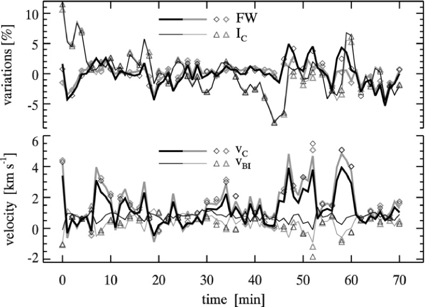
Figure 10: Temporal evolution of the fit width FW, the core intensity $I_{\rm C}$, the core velocity $v_{\rm C}$, and the bisector velocity $v_{\rm BI}$ of the line core fit of the H$\alpha$ spectral line in the network element (Figs. 4–7) derived by the $4^{\rm th}$-order polynomial. FW and $I_{\rm C}$ are shown as variations with respect to their temporal means (top panel). Positive $v_{\rm C}$ and $v_{\rm BI}$ signalize a redshift (middle and bottom panel). Gray and black lines indicate the uncorrected and corrected characteristics, respectively, derived from spatial means of the intensities. Gray and black symbols shown with the time step of 2 min indicate the uncorrected and corrected characteristics, respectively, derived as spatial means of particular values at each pixel.

5.1 Temporal evolution of the spectral characteristics

The top panel of Fig. 10 shows temporal evolutions of the relative variations of the fit width FW and the core intensity $I_{\rm C}$ of the line core fits of the H$\alpha$ spectral line in the network element (Figs. 4–7) with respect to their temporal means. The bottom panel shows temporal evolutions of the core velocity $v_{\rm C}$ and the bisector velocity $v_{\rm BI}$, whose positive values indicate redshift and redward asymmetry of the line core. All these characteristics were derived from the original H$\alpha$ datacubes downloaded from the DOT database. An application of the corrections (Paper I) increases apparently the amplitude of the FW variations after the $40^{\rm th}$ min, but decreases both velocities within the whole 71-min period. The values of FW and $I_{\rm C}$ seem to be largely insensitive to the choice of averaging for the size of the selected area, but this is not the case of $v_{\rm C}$ and $v_{\rm BI}$. Their corrected values resulting from spatial averaging over the network element (black diamonds and triangles in the bottom panel) differ systematically from the values inferred from spatial means of the intensities (black thick and thin lines). This is probably due to high non-linearity of the respective correcting functions shown in Paper I. The temporal evolutions of the characteristics do not show any apparent systematic trend and fast short-period variations dominate them. The variations of corrected FW are within the range $\pm 5$ % around the mean. The variations of $I_{\rm C}$ indicate a rapid darkening of the selected network element (Fig. 4) from 11 % above an average to average within the first 10 minutes. Later on, $I_{\rm C}$ variations lie within the range from $-9$ % to $+6$ %. The corrected $v_{\rm C}$ displays redshifts up to 4 km s^-1, with an average of 1.5 km s^-1 and a noticeable correlation with the corrected FW, most apparent after the fortieth minute. In the same period, a large expanding granule with the maximum diameter larger than 2 arcsec appeared in the low photosphere (see Figs. 6 and 7). Fig. 10 suggests also some similarity between the $v_{\rm C}$ and $I_{\rm C}$ variations. The Fourier cross correlation indicates that $I_{\rm C}$ lags behind $v_{\rm C}$ about 2.1 min on average. The H$\alpha$ core possesses mostly a redward asymmetry corresponding to an inverse-C bisector with the average bisector velocity of about 0.5 km s^-1 with excursions up to 1 km s^-1.

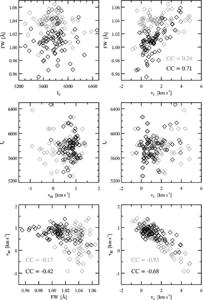
Figure 11: Scatter plots of the spectral characteristics shown in Fig. 10 – the case of spatial means of the intensities. Gray and black symbols indicate the uncorrected and corrected characteristics, respectively. Unlike Fig. 10, the plots show absolute values of FW and $I_{\rm C}$. Positive $v_{\rm C}$ and $v_{\rm BI}$ signalize a redshift. There are also shown the correlation coefficients CC for the pairs FW – $v_{\rm C}$, $v_{\rm BI}$ – FW, and $v_{\rm BI}$ – $v_{\rm C}$ for uncorrected (gray) and the corrected (black) values.

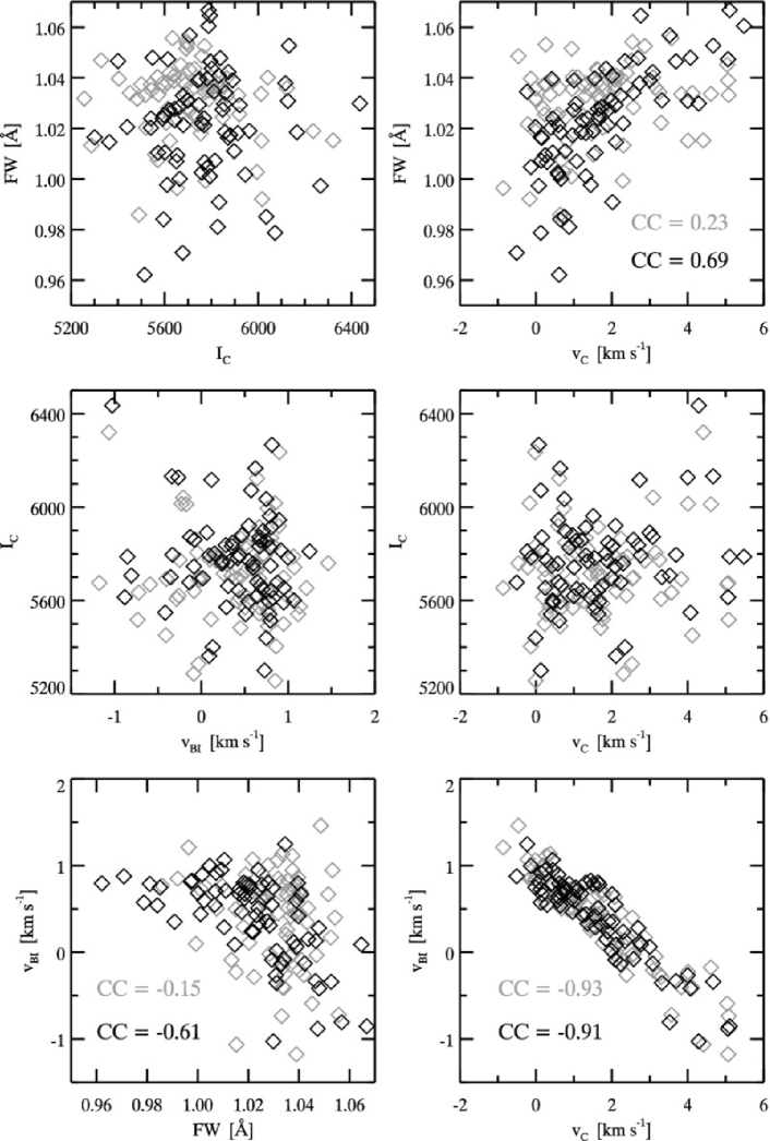
Figure 12: Scatter plots of the spectral characteristics shown in Fig. 10 – the case of spatial means of the spectral characteristics at each pixel. Gray and black symbols indicate the uncorrected and corrected characteristics, respectively. Unlike Fig. 10, the plots show absolute values of FW and $I_{\rm C}$. Positive $v_{\rm C}$ and $v_{\rm BI}$ signalize a redshift. There are also shown the correlation coefficients CC for the pairs FW – $v_{\rm C}$, $v_{\rm BI}$ – FW, and $v_{\rm BI}$ – $v_{\rm C}$ for the uncorrected (gray) and corrected (black) values.

5.2 Scatter plots

The spectral characteristics from Fig. 10 are displayed in the form of scatter plots in Figs. 11 and 12, showing separately the results of spatial averaging of the intensities and the spectral characteristics at each pixel, respectively. The top left panels show FW against $I_{\rm C}$ which do not correlate, neither uncorrected nor corrected. The top right panels suggest a positive correlation between FW and $v_{\rm C}$, which occurs only for the corrected values. The correlation implies that more redshifted profiles tend to be wider. The middle panels indicate that there is no apparent correspondence between $I_{\rm C}$ and the velocities. The values of $I_{\rm C}$ do not correlate with $v_{\rm C}$, not even after shifting $I_{\rm C}$ forward (i.e., to the left with respect to the zero of the time axis) about 2.1 min to compensate its apparent lag indicated in Fig. 10. The bottom left panel of Fig. 12 suggests an anticorrelation between $v_{\rm BI}$ and FW, which occurs only for the corrected values resulting from their spatial averaging at each pixel. The anticorrelation implies that while narrower H$\alpha$ cores display a redward asymmetry, the wider and more redshifted profiles (see the FW – $v_{\rm C}$ correlation above) display a blueward asymmetry. The bottom right panels also suggest a striking anticorrelation between $v_{\rm BI}$ and $v_{\rm C}$. Notably, the profiles with the zero Dopplershift display a redward asymmetry with $v_{\rm BI}$ = 1 km s^-1 and become symmetric for $v_{\rm C}$ of 2 km s^-1, but tend to display an increasing blueward asymmetry with further-increasing redshift.

6 Discussion

We derived spectral characteristics of the H$\alpha$ spectral line observed in the network element with the aim of seeking signatures of the Alfvén waves as reported in Jess et al. (2009). How do our findings compare to the results of these authors? While Jess et al. (2009) reported an average blueshift of 23 km s^-1 in a cluster of bright points seen in H$\alpha$, we found an average redshift of about 1.5 km s^-1. Obviously, this is a large discrepancy and we suspect that our particular choice of the reference wavelength of the core velocity might be partially responsible for that. We remind that we made no distinction between the network and internetwork (see Section 3). But as we showed in Section 4, selecting only internetwork areas shifts the reference wavelength blueward only insignificantly up to 0.2 km s^-1 and the value of the average redshift is significantly above the uncertainty of 0.3 km s^-1 of the reference wavelength. Further, Jess et al. (2009) reported an absence of any significant intensity variations in the cluster of bright points. However, there is some uncertainty whether they refer to the spectral intensity in the line core, or the integrated intensity. Our results suggest that the core width variations in the selected network element are associated with both the core velocity and core intensity variations. Finally, the authors detected FWHM oscillations of the H$\alpha$ spectral line with the strongest power in the 400-to-500 s interval. We postpone detailed cross correlation, Fourier, and wavelet analyzes of our results to a forthcoming paper. We conclude that, most likely, a different mechanism works in the selected network element than in the cluster of the bright points studied by Jess et al. (2009). The inverse-C bisector and the average redshift of the H$\alpha$ line core are more symptomatic for propagation of chromospheric shocks, as suggested in Uitenbroek (2006) and demonstrated in numerical simulations by Heggland et al. (2011). Then the lagging of the core intensity $I_{\rm C}$ behind the core velocity $v_{\rm C}$ variations about 2.1 min might be characteristic either for the p-mode oscillations leaking into the chromosphere, or for the shock wave propagation. Although there is an apparent similarity of their variations best seen after the fortieth minute (Fig. 10), shifting $I_{\rm C}$ forward about the 2-min lag does not improve the $I_{\rm C}$ – $v_{\rm C}$ correlations shown in the middle right panels of the scatter plots in Figs. 11 and 12, which may be ascribed to a variable phase shift which varies in time and/or frequency.

Since the standard DOT observations do not involve any precise wavelength calibration of the H$\alpha$ filtergrams, we refrained from interpreting straightforwardly redshifts and blueshifts as actual mass downflows and upflows, respectively. Despite these facts, we will try to reason that most of the positive values of $v_{\rm C}$ indicated by the redshifts of the H$\alpha$ core may represent the actual mass downflows. As we noted in Section 2, the zero wavelength of the filtergrams is centered on the minimum of an average profile taken before the observations over the field of view. Thus, the zero wavelength approximately corresponds to the H$\alpha$ solar disc-center wavelength of $\lambda_{\rm sol}=6562.81$ Å according to the spectral FTS atlas by Neckel (1999), whose wavelength scale was already corrected for the rotational and radial velocity of the Earth. Consequently, the reference wavelength given in Section 3 corresponds to $\lambda_{\rm R}=\lambda_{\rm sol}-0.018$ Å = 6562.79 Å. The local standard of rest at the solar surface for the H$\alpha$ spectral line is: $\lambda_{0}=\lambda_{\rm lab}(1+v_{\rm GR}/c)=6562.80$ Å, where $\lambda_{\rm lab}=6562.79$ Å is the air laboratory wavelength of H$\alpha$ adopted from the NIST database (Kramida et. al, 2012), $v_{\rm GR}=0.636$ km s^-1 is the solar gravitational redshift, and $c$ is the speed of light. Then the core velocities of H$\alpha$ measured within this study are offset only about $(\lambda_{0}-\lambda_{\rm R})c/\lambda_{0}=0.5$ km s^-1 with respect to the local standard of rest at the target area, with the following consequences:

• the zero of $v_{\rm C}$ and all values of $v_{\rm BI}$ in Fig. 10 should be shifted redward (i.e., up) about 0.5 km s^-1,

• the zeros of the $v_{\rm C}$ axes in Figs. 11 and 12 should be shifted redward (i.e., to the right) about 0.5 km s^-1,

• most of the positive values of $v_{\rm C}$ indicated by the redshifts of the H$\alpha$ core may represent the actual mass downflows.

7 Conclusions

A selected network element exhibits distinct spectral characteristics seen in their temporal evolutions and scatter plots correlating pairs of values from the same instant. In general, this involves:

• the fit width variations about $\pm 5$ %, i.e., a few tens of milliångströms with respect to the average of 1.01 Å,

• the core intensity variations about $\pm 10$ % with respect to the average,

• the core velocity variations from 0 to 4 km s^-1 about the average of 1.5 km s^-1, implying a redshift,

• the core asymmetry variations of the H$\alpha$ line core up to 1 km s^-1 about the average of 0.5 km s^-1, suggesting an inverse-C bisector.

The H$\alpha$ core width tends to correlate with the Dopplershift and anticorrelate with the asymmetry, suggesting that more redshifted H$\alpha$ profiles are wider and the broadening of the H$\alpha$ core is accompanied with a change of the core asymmetry from redward to blueward. We found also a striking anticorrelation between the core asymmetry and the Dopplershift, suggesting also a change of the core asymmetry from redward to blueward, with an increasing redshift of the H$\alpha$ core. A question is which of these patterns are unique just for the network and which are also common in the internetwork. This can be resolved in a stand-alone study, comparing the spectral characteristics of the H$\alpha$ line in the network and internetwork. Finally, an absence of blueshift and detected intensity and velocity variations probably exclude a presence of Alfvén waves in the selected network element according to the criteria given in Jess et al. (2009).

- [1] Mathioudakis, M., Jess, D.B., Erdélyi, R.: 2012, Space Sci. Rev., Online First, 94 \articleNeckel, H1999\sph184421 \articleOsterbrock, D.E.1961ApJ134347 \articleRutten, R.J., Hammerschlag, R.H., Bettonvil, F.C.M., Sütterlin, P., de Wijn, A.G.2004\aaa4131183 \articleSchoolman, S.A.1972\sph22344 \articleUitenbroek, H.2006ApJ639516