From Forbidden Coronal Lines to Meaningful Coronal Magnetic Fields

Abstract

We review methods to measure magnetic fields within the corona using the polarized light in magnetic-dipole (M1) lines. We are particularly interested in both the global magnetic-field evolution over a solar cycle, and the local storage of magnetic free energy within coronal plasmas. We address commonly held skepticisms concerning angular ambiguities and line-of-sight confusion. We argue that ambiguities are in principle no worse than more familiar remotely sensed photospheric vector-fields, and that the diagnosis of M1 line data would benefit from simultaneous observations of EUV lines. Based on calculations and data from eclipses, we discuss the most promising lines and different approaches that might be used. We point to the S-like [Fe XI] line (J=2 to J=1) at 789.2nm as a prime target line (for ATST for example) to augment the hotter 1074.7 and 1079.8 nm Si-like lines of [Fe XIII] currently observed by the Coronal Multi-channel Polarimeter (CoMP). Significant breakthroughs will be made possible with the new generation of coronagraphs, in three distinct ways: (i) through single point inversions (which encompasses also the analysis of MHD wave modes), (ii) using direct comparisons of synthetic MHD or force-free models with polarization data, and (iii) using tomographic techniques.

1 Introduction

s:Introduction

Measurement of solar magnetic-fields has been a goal of solar physics since the discovery of the Zeeman effect in sunspots by Hale (1908). Our purpose here is to review how magnetic-dipole (M1) lines, formed in coronal plasma, might be used to address particular questions in coronal and heliospheric physics: How does the coronal magnetic-field vector evolve over the solar sunspot cycle? Can we measure some of the free magnetic energy on observable scales in the corona, and its changes, say, before and after a flare?

Theoretical work by Charvin (1965) spurred experimental studies of the polarization of magnetic-dipole lines, such as [Fe XIII] $3p^{2}\ {}^{3}\!P_{1}\rightarrow 3p^{2}\ {}^{3}\!P_{0}$ at 1074.7 nm, as a way to constrain coronal magnetic-fields. The lines are optically thin in the corona; their intensities are $\lesssim 10^{-5}$ of the disk continuum intensities. Thus they can be observed only during eclipses or using coronagraphs that occult the solar disk.

Here, we review M1 emission-line polarization towards the specific goal of measuring the vector magnetic-field $[{\bf B}({\bf r};t)]$ throughout a sub-volume of the corona. To date, this has not been achieved. We have little idea of the true origin of CMEs, flares, and coronal heating. even though coronal plasma has been regularly observed since the 1930s. The latest of several decades of high-cadence images of coronal plasma from space reveal more details but are limited to studying effects, not causes, of coronal dynamics, since such instruments measure thermal, not magnetic, properties. To discover the cause of coronal dynamics we must measure ${\bf B}({\bf r};t)$ above the photosphere- the region of the atmosphere where free energy is stored and quickly released, since it is the free energy associated with electrical current systems within coronal plasmas that drives these phenomena. Measurements of ${\bf B}({\bf r};t)$ in the photosphere have been done for decades, but photospheric dynamics occurs under mixed $\beta$ conditions ($\beta=$ gas/magnetic pressure $\approx 1$). In contrast, the low-$\beta$ coronal plasma should exist in simpler magnetic configurations, perhaps more amenable to straightforward interpretation. In MHD the electrical currents are simply ${\bf j}={\rm curl}~{}{\bf B}({\bf r};t)$. Given sufficiently accurate measurements of ${\bf B}({\bf r};t)$ in the low-$\beta$ corona, both ${\bf j}$ and the free energy itself can in principle be derived.

Like all observational studies, this is bandwidth-limited exercise. We can investigate structures only from the smallest resolvable scales $\ell$ to the largest $\approx{\rm R}_{\odot}\approx 700$ Mm, and on time scales longer than the smallest time $\tau$ needed to acquire the data. The spatial range will be limited by forseeable observational capabilities to $\ell\gtrsim 1$Mm. Successful tomographic-inversions using solar rotation to slice through the 3D corona require $\tau\gtrsim 1$ day, during which the corona is viewed from angles differing by $\approx 1/4$ radian. Given our goal, it is clear that we will not be able to investigate either the dissipation scales of magnetic-fields, nor changes in magnetic-fields on rapid dynamical time scales $\lesssim{\rm R}_{\odot}/C_{A}\approx 350$ s of the inner corona (here $C_{A}\approx 2$ Mm s^-1 is the Alfvén speed). However, these limitations are not new. In any case coronal dynamics and flares involve a slow build-up and sudden release of magnetic free energy (Gold and Hoyle, 1960). This energy build-up can indeed, and should be, explored through new measurements of ${\bf B}({\bf r};t)$.

2 The Inverse Problem

sec:inversion

2.1 General Considerations

Consider a heliocentric coordinate system with Sun center at ${\bf r}\equiv(x,y,z)^{T}={\bf 0}$, with the line of sight along $z$, and $x,y$ being in the plane of the sky. Given a set of observations $\left[\{I_{i\ldots 4,\nu}(x,y,t)\}\right]$ of the four Stokes parameters [$IQUV$] at $n$ frequencies $[\nu]$ across a M1 line at time $t$, we seek solutions for ${\bf B}(x,y,z;t)$ over an observable sub-volume of the corona $\approx\Delta x\Delta y\Delta z$. We can write

$$\ilabel{eq:forward}I_{i,\nu}(x,y;t)=\int_{\Delta z}\varepsilon_{i}({\bf S}({\bf r};t))\,{\rm d}z=\Phi_{i}({\bf S}({\bf r};t)).$$ (1)

The M1 lines – having small oscillator strengths – are optically thin through the corona. Under these conditions $\varepsilon_{i}$ is a non-linear, but local function of a “source vector” $S_{j},j=1\ldots n$. The price for “optical thinness” is that $\Delta z$ encompasses the entire line of sight through the corona to the solar disk or into space. Tomography specifically takes advantage of this. There is, however, skepticism in the community concerning the magnetic-field measurements under optically thin conditions that we address in Section s:LOS. The non-linearity arises because the Stokes parameters ${\bf I}$ depend on the “atomic alignment” [$\sigma^{2}_{0}(\alpha_{0}J)$], a scalar quantity that is a linear combination of magnetic-substate populations. The alignment can be positive, negative, or zero, as discussed below. Ignoring the alignment would make the problem linear in the source term (like the standard emission measure problem for line intensities only).

The source [${\bf S}$] must be written as a function of ${\bf r}$ and time [$t$] in terms of necessary thermodynamic and magnetic parameters. At a minimum this means specifying

$${\bf S({\bf r};t)}=\left\{\rho({\bf r};t),{\bf v({\bf r};t)},T({\bf r};t),{\bf B}({\bf r};t)\right\},$$

for plasma with density $\rho$ moving with velocity ${\bf v}$ at temperature $T$. These quantities must be supplemented by calculations that give the local distributions of ionization states and electron density. Any formal “inverse” solution is of the form

$$\ilabel{eq:inverse}{\bf S}({\bf r};t)=\Phi^{-1}{\bf I}(x,y;t),$$ (2)

where ${\bf I}$ is the $4n$-long “vector” of observed Stokes parameters. Clearly, a 3D array of scalar and vector-fields such as ${\bf S}({\bf r};t)$ cannot be recovered from one set of measurements [${\bf I}(x,y;t)$] that are integrated over $\Delta z$. Additional information is needed.

A “good diagnostic” maps components of ${\bf I}$ into ${\bf S}$. If Equation (eq:forward) were linear (or were linearized) we could write (e.g., Craig and Brown, 1986)

$$\ilabel{eq:cb}{\bf S}={\bf\left(\Phi^{T}\Phi\right)}^{-1}{\bf\Phi^{T}\ I}.$$ (3)

The eigen-spectrum of matrix ${\bf\left(\Phi^{T}\Phi\right)}^{-1}$ measures the degree to which measurements of ${\bf I}$ can be used to determine ${\bf S}$. As usual, the formal operation given by Equation (eq:cb) should not be taken as an inverse solution, it is ill-posed (Craig and Brown, 1986).

2.2 Origin of Polarization of Magnetic-Dipole Coronal Lines

s:info

Polarization of spectral lines is generated in two ways (e.g., Casini and Landi Degl’Innocenti, 2008). Any process that produces unequal sub-level populations, such as anisotropy of illuminating radiation, also produces polarization of light in the emitted radiative transitions to/from a given atomic level. When magnetic-substate populations are equal, the state is “naturally populated” and light is unpolarized. The second way is to separate the substates in energy, so that spectroscopy can discriminate states of polarized light associated with the specific changes in energy of states with different sub-level quantum numbers $[M]$, no matter how the sub-levels are populated. Magnetic- and electric- fields thus are imprinted on spectral line polarization through the Zeeman and Stark effects. Since charge neutrality is a good approximation in coronal plasma (e.g. Parker, 2007), electric-fields and the associated stresses are far smaller than those for the magnetic-field, and in quasi-static situations can be ignored. We focus on the magnetic-fields.

Adopting the notation of Casini and Judge (1999), for M1 emission-lines between upper- and lower-levels with quantum numbers $\alpha J$ ($J=$ total angular momentum) and $\alpha_{0}J_{0}$, the $\varepsilon_{i}$ terms in Equation (eq:forward) are proportional to a term of the form

$$\epsilon_{JJ_{0}}={{h\nu}\over 4\pi}\,N_{\alpha_{0}J}\,A_{\alpha_{0}J\to\alpha_{0}J_{0}}.$$ (4)

This term is simply the emission coefficient (ignoring stimulated emission) for the unpolarized transfer problem, in units of erg cm^-3 sr^-1 s^-1. The population density of the upper-level can be factored as usual as

$$N_{\alpha_{0}J}\, = \frac{N_{\alpha_{0}J}\,}{N_{ion}}\,\frac{N_{ion}}{N_{el}}\,\frac{N_{el}}{N_{H}}\,\frac{N_{H}}{n_{\rm e}}\,n_{\rm e}\,.$$ (5)

We label the first factor on the RHS of the above equation $f$, it is the ratio of the upper-level population of the level emitting the photons to the total ion population. The remaining factors are, in order, the ionization fraction, element abundance, ratio of hydrogen nuclei number density to the electron number density $n_{\rm e}$, and lastly $n_{\rm e}$ itself. For strong lines (electric dipole or “E1” lines in the EUV/ soft X rays) $f\propto n_{\rm e}$ and $\exp(-h\nu/kT)$, so that $N_{\alpha_{0}J}\propto n_{\rm e}^{2}G(T)$ as usual. For M1 lines $f\propto n_{\rm e}^{\beta}$ with $0<\beta<1$, but generally $h\nu/kT\ll 1$, so the temperature dependence of $N_{\alpha_{0}J}$ enters mostly the ionization fraction. Under coronal ionization equilibrium conditions this factor is a function only of temperature $T$.

The polarized terms [$\varepsilon_{i}$] also depend on the anisotropy of the incident photospheric radiation, particle collisions, the strength and direction of the coronal magnetic-field, and the direction of the line of sight. M1 lines have large radiative lifetimes ($\tau_{R}\approx A_{\alpha_{0}J\to\alpha_{0}J_{0}}^{-1}\approx 10^{-1}$s). The Larmor frequency [$\nu_{\rm L}\approx\mu_{B}B/h$] is much larger than the inverse lifetime of the level, $\nu_{\rm L}\tau_{R}\gg 1$. This is the “strong field” (or “saturation”) limit of the Hanle effect. If the photospheric irradiation is rotationally symmetric and spectrally flat, the atomic polarization is in the special form of alignment [$\sigma^{2}_{0}(\alpha_{0}J)$] which in terms of substate populations is written

eqn:alignpop$$\sigma^{2}_{0}(\alpha J) = {\sqrt{5}\over\sqrt{J(J+1)(2J-1)(2J+3)}}\sum_{M}[3M^{2}-J(J+1)]\,\frac{N(\alpha_{0}{\scriptstyle JM})}{N(\alpha_{0}{\scriptstyle J})}$$ (7)

Circularly polarized light is generated only by the “$\sigma$”-components ($\Delta M=\pm 1$) of the Zeeman effect. The M1 emission coefficients $\varepsilon_{i}^{(j)}$ for Stokes parameter $i$ are (Section 4 of Casini and Judge, 1999):

$$\varepsilon_{0}^{(0)}(\nu,\hat{\bf k}) = \epsilon_{JJ_{0}}\,\phi(\nu_{0}-\nu)\left[1+D_{JJ_{0}}\,\sigma^{2}_{0}(\alpha_{0}J)\,{\cal T}^{2}_{0}(0,\hat{\bf k})\right]\;,$$ (8)

$$\varepsilon_{i}^{(0)}(\nu,\hat{\bf k}) = \epsilon_{JJ_{0}}\,\phi(\nu_{0}-\nu)\,D_{JJ_{0}}\,\sigma^{2}_{0}(\alpha_{0}J)\,{\cal T}^{2}_{0}(i,\hat{\bf k})\;,\qquad(i=1,2)$$ (9)

$$\varepsilon_{3}^{(1)}(\nu,\hat{\bf k}) = -{\textstyle\sqrt{2\over 3}}\,\nu_{\rm L}\,\epsilon_{JJ_{0}}\,\phi^{\prime}(\nu_{0}-\nu)\left[\bar{g}_{\alpha_{0}J,\alpha_{0}J_{0}}+E_{JJ_{0}}\,\sigma^{2}_{0}(\alpha_{0}J)\right]{\cal T}^{1}_{0}(3,\hat{\bf k}),$$ (10)

where $j$ in $\varepsilon_{i}^{(j)}$ is the leading order in the Taylor series expansion of the emission coefficient with frequency. $\phi(\nu_{0}-\nu)$ is the line profile [Hz^-1], $\phi^{\prime}(\nu_{0}-\nu)$ its first derivative with respect to $\nu$, remaining terms (except $\nu_{\rm L}$) are dimensionless. The factor $D_{JJ_{0}}$ depends only on angular momenta and $E_{JJ_{0}}$ also depends on the Landé g-factor of the transition: $\bar{g}_{\alpha_{0}J,\alpha_{0}J_{0}}$. The tensor ${\cal T}^{1,2}_{0}(i,\hat{\bf k})$ relates the angular distribution and polarization of emitted radiation to the direction of the observer. In terms of angles $\gamma_{B}$ and $\Theta_{B}$ defining the magnetic azimuth in the plane-of-the-sky and inclination along the line-of-sight, these are

${\cal T}^{2}_{0}(0,\hat{\bf k})_{\rm M1}$	=	${\textstyle{1\over 2\sqrt{2}}}(3\cos^{2}\!\Theta_{B}-1)$
${\cal T}^{2}_{0}(1,\hat{\bf k})_{\rm M1}$	=	${\textstyle{3\over 2\sqrt{2}}}\cos 2\gamma_{B}\sin^{2}\!\Theta_{B}$
${\cal T}^{2}_{0}(2,\hat{\bf k})_{\rm M1}$	=	$-{\textstyle{3\over 2\sqrt{2}}}\sin 2\gamma_{B}\sin^{2}\!\Theta_{B}$
${\cal T}^{1}_{0}(3,\hat{\bf k})_{\rm M1}$	=	${\textstyle\sqrt{3\over 2}}\cos\Theta_{B}$.

2.3 M1 Lines From One Point in the Corona

Sometimes coronal images are dominated by emission from one small region, such as from a small section of an active region loop at ${\bf r_{0}}=(x_{0},y_{0},z_{0})^{T}$. In this case the source ${\bf S}({\bf r};t)\,={\bf S}(t)\delta(x-x_{0})\delta(y-y_{0})\delta(z-z_{0})$ and the measured I is simply $\propto\varepsilon_{i}^{(j)}$ evaluated at ${\bf r}=(x_{0},y_{0},z_{0})^{T}$. By inspection of expressions for $\varepsilon_{i}$ we see that

1. The magnetic-field strength is encoded only in circular polarization through $\varepsilon_{3}^{(1)}(\nu,\hat{\bf k})$, via $\nu_{\rm L}$, and only as the product $B\cos\Theta_{B}$.

2. The usual weak-field “magnetograph formula” – taking the ratio of Equation (eqn:eps31) and the derivative of Equation (eqn:eps00) – does not only depend on the Landé g-factor $\bar{g}_{\alpha_{0}J,\alpha_{0}J_{0}}$. In the presence of a non-zero alignment, the ratio includes smaller terms including $\sigma^{2}_{0}(\alpha_{0}J)$ in both numerator and denominator.

3. The magnetic-field azimuth $\gamma_{B}$ is encoded in the linear polarization as $\gamma_{B}=$ $-\frac{1}{2}\arctan(\varepsilon_{2}^{0}/\varepsilon_{1}^{0})$.

Of course, in reality, measured quantities [I] are integrals of these elementary $\varepsilon_{i}^{(j)}$ coefficients along the line of sight.

2.4 “Long” Line of Sight Integrations

s:LOS

A concern sometimes expressed among solar physicists is that M1 coronal emission-lines form over such large distances that they have limited use in diagnosing magnetic-fields. The perceived problem is that the magnetic-field changes too much along the long lines of sight $L_{c}\approx{\rm R}_{\odot}$. Mathematically we might say

$${\ilabel{e:scales}}\left|\frac{\partial B_{i}}{\partial s}\right|L_{c}\gtrsim|\langle B_{i}\rangle|,$$ (11)

for magnetic vector component $B_{i}$.

Let us apply the same arguments to a familiar situation in which there is far less such preconceived skepticism: the solar photosphere. It is indeed a “thin” layer (500 km) compare with the solar radius, but this does not mean that it is “thin” (small $L_{\rm c}$) in the sense implied by Equation (e:scales). Photospheric magnetic-fields are highly intermittent in space and time. Consider formation of polarized light from a simple cylindrical “flux tube” of diameter 160 km in the solar photosphere (e.g. Steiner, 1994, left panel of Figure fig:ftcor). The photon mean free path [mfp] in the photosphere $L_{p}\approx H_{p}$ is $\approx 120$ km, as indicated by “mfp”. Clearly there is structure in the thermal and magnetic conditions well below the photon mfp. As discussed by Steiner and others, this leads to “peculiar” Stokes profiles – the “Stokes-$V$ area asymmetry” being one parameter of particular interest. The point here is not that peculiar Stokes profiles can be explained, but that in photospheric problems of interest, one must diagnose magnetic-fields in situations the inequality in Equation (e:scales) holds!

Consider next the second panel of Figure fig:ftcor, showing rays through an image of the corona during eclipse. The rays intercept many different structures, and again the condition in Equation (e:scales) applies. But this image mis-represents the LOS confusion because the structures shown are already integrated along the orthogonal LOS (in and out of the page). In 3D, the actual rays will intercept far fewer of these structures than is suggested by this image. It is by no means clear that the LOS integration is worse in the corona than in the photosphere, when it comes to trying to diagnose magnetic fields of interest.

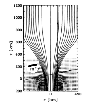
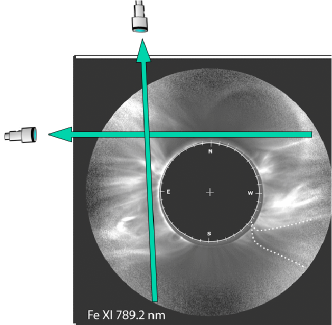
Figure 1.: Left: magnetic-field lines and velocity vectors for a flux tube extending from beneath the photosphere into the chromosphere, from Steiner (1994) but annotated with the photon mean free path. Two rays intercepting the boundary between magnetised plasma are shown, along which spectral lines are formed. Right: an image of the corona during the July 2011 eclipse in the Fe XI 789.2 nm line is shown, obtained by one of us (SH). Two integration rays are shown. Note that this image already has been integrated in one dimension, thus in 3D such rays intercept much less structure than this image might seem to suggest. fig:ftcor

2.5 Atomic Alignment

sec:align

A proper interpretation of M1 emission-lines requires knowledge of $\sigma^{2}_{0}(\alpha_{0}J)$, in an inversion it must be solved for as part of the solution for ${\bf S}({\bf r};t)$ (Judge, 2007). The alignment comes from solutions to atomic sub-level population calculations. Even in statistical-equilibrium, the equations are non-linear coupled multi-level systems requiring numerical solution. This presents a problem for inversions since this expands the solution space to include the alignment itself, which becomes non linear in the source parameters ${\bf S}({\bf r};t)=\left\{\rho({\bf r};t),{\bf v({\bf r};t)},T({\bf r};t),{\bf B}({\bf r};t)\right\}$.

To understand the non-linearities we can consider atomic models of increasing complexity. First consider a two–level atomic model for a $J=1\rightarrow J_{0}=0$ transition excited only by photospheric radiation, for which analytic solutions are available from, e.g., Casini and Landi Degl’Innocenti (2008). Their Equation 12.23 gives

$$\ilabel{eqn:twol}\sigma_{0}^{2}(1)=\frac{w}{2\sqrt{2}}\left(3\cos^{2}\vartheta_{B}-1\right),\ \ {\rm(two\ level\ atom},\ J=1\rightarrow J_{0}=0)$$ (12)

where $w$ measures the radiation anisotropy. Here, $\vartheta_{B}$ (different from $\Theta_{B}$) measures the local angle between the magnetic-field vector and solar gravity vector (central axis of the radiation cone). When the center-to-limb variation of the intensity is zero, $w=\frac{1}{2}(1+\cos\vartheta_{M})\cos\vartheta_{M}$ ($\vartheta_{M}$ is the angle subtended by the solar radius at a point [${\bf r}$] in the corona). In this case the alignment is generated by anisotropic but rotationally symmetric radiation in the transition itself.

The magnitude of alignment is reduced by processes tending to populate sub-levels naturally, making $\frac{N(\alpha_{0}{\scriptstyle JM})}{N(\alpha_{0}{\scriptstyle J})}\rightarrow 1/(2J+1)$ and so $|\sigma^{2}_{0}(\alpha J)|\rightarrow 0$ in Equation (eqn:alignpop). Collisions with particles having isotropic distribution functions thus reduce the magnitude of any existing alignment. Such collisions tend to leave the angular dependence of existing alignment essentially unchanged. This result is demonstrated through the multi-level calculations for Fe XIII by Judge (2007), where the alignment of the upper-levels ($3p^{2}\,{}^{3}\!P_{J=2,1}$) of the 1074.7 and 1079.8 nm lines of Fe XIII were found to factorize as

$$\ilabel{eqn:alignf0}\sigma^{2}_{0}(\alpha_{0}J)\approx k_{J}(T_{\rm e},n_{\rm e},\vartheta_{\rm M})\,{1\over 2}(3\cos^{2}\vartheta_{\rm B}-1)\,,$$ (13)

to within $0.7\,\%$ and $3.2\,\%$ respectively. The level-dependent term $k_{J}(T_{\rm e},n_{\rm e},\vartheta_{\rm M})$, an approximate generalization of the factor $\frac{w}{\sqrt{2}}$ in Eq. (eqn:twol), is a positive definite factor depending only on local thermal conditions and the nature of the disk irradiation through $\vartheta_{\rm M}$. It is not linear in any of these variables. The factor $k_{J}(T_{\rm e},n_{\rm e},\vartheta_{\rm M})$ thus determines the magnitude of the alignment for any orientation of the coronal magnetic field given by the other factor in variable $\vartheta_{\rm B}$. In Equations (eqn:eps00) and (eqn:eps31) it enters expressions for Stokes-$I$ and $V$ only as small first order corrections that leave the signs of these terms unchanged.

As a general rule the magnitude of $k_{J}(T_{\rm e},n_{\rm e},\vartheta_{\rm M})$ is smaller for larger values of $J$, since the number of sub states [$2J+1$] is larger. Thus the 1079.8 nm transition of Fe XIII ($J=2\rightarrow J=1$) has a smaller linear polarization than the 1074.7 nm ($J=1\rightarrow 0$) transition. Transitions such as 1079.8 nm with small $k_{J}(T_{\rm e},n_{\rm e},\vartheta_{\rm M})$ will therefore be useful since then the non-linear terms are commensurately smaller in the Stokes-$I$ and $V$ parameters.

For the $J=1$ level, Equation (eqn:twol) represents an upper limit to Equation (eqn:alignf0), a limit which applies when collisions are negligible (e.g., $n_{\rm e}\rightarrow 0$). The alignment generated by anisotropic irradiation is reduced by sum of all the collisions coupling the $J=1$ sub-levels to others in the 26-level atom. This behavior is expected in many other M1 lines of interest.

If the alignment can be shown to be zero, there is no linear polarization and only the Stokes-$I$, $V$ profiles can be used to get a “standard” line-of-sight magnetogram for $B\cos\Theta$. If it is finite, it can take either sign because of the factor $(3\cos^{2}\vartheta_{B}-1)$, and it leads directly to linear polarization. Observed minima in linear polarization, obtained for example with the Coronal Multi-channel Polarimeter [CoMP] (Tomczyk et al., 2008), often reflect the Van Vleck condition $(3\cos^{2}\vartheta_{B}=1)$, giving a direct indication of part of the magnetic-field’s geometry. Passing across such minima one finds a 90^∘ change in direction of the linear polarization vector as $(3\cos^{2}\vartheta_{B}-1)$ and the alignment changes sign, according to Equation (eqn:epsi0). This is a tell-tale sign of the Van Vleck effect even under the presence of significant intergrations along the line-of-sight (LOS).

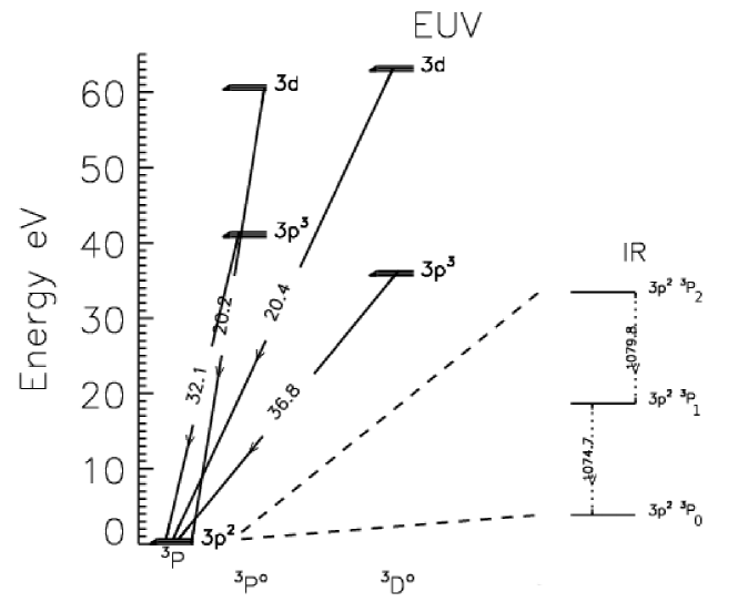
Figure 2.: Term diagram for Fe XIII showing the strongest E1 transitions of each multiplet, and the M1 lines among the levels of the ground term. The 1074.7 nm line has upper-level $J=1$, lower $J=0$. Each configuration shown has EUV line ratios sensitive to density and photospheric radiation field as a result of the competition for sub-level populations in the ground term. fig:fe13˙td

With these arguments we can summarize the role of the alignment as follows (e.g. Judge, 2007):

1. The magnetic-field azimuth has the well-known $90^{\circ}$ ambiguity, unless the sign of $\sigma^{2}_{0}(\alpha_{0}J)$ can be determined, in which case there remains a 180^∘ ambiguity.

2. The magnitude and sign of the alignment $\sigma^{2}_{0}(\alpha_{0}J)$ affects all four Stokes parameters.

3. Measurements of electron-density-sensitive lines at IR and EUV wavelengths will help determine $|\sigma^{2}_{0}(\alpha_{0}J)|$ and should be included as part of the vector of observables ${\bf I}$.

4. Measurements of M1 lines from $J>1$ levels (e.g. Fe XI 782.9 nm, Fe XIII 1079.8 nm) with their smaller alignment $|\sigma^{2}_{0}(\alpha_{0}J)|$, will make inversions more linear. In comparison with strongly aligned transitions (Fe XIII 1074.7 nm for example), such transitions have smaller $|\sigma^{2}_{0}(\alpha_{0}J)|$ non-linear factors for $I$ and $V$ in Equations (eqn:eps00) and (eqn:eps31).

2.6 Selection of Lines for Inversion

Judge (2007) has examined how the alignment might be constrained – even determined – from observations, in the simplest case where a single point dominates all emission from an M1 coronal line. For a given set of such measurements [I], he has shown that there are generally multiple roots to the governing Equations for the atomic alignment. The solutions correspond to different scattering geometries that are compatible with data (see his Table 2). Even in principle there is no unique solution.

Table 1.: An example of a set of lines in Fe XIII for magnetic inversionstbl:1

$\lambda$	Type	Data	Transition and Comments
[nm]		needed
1074.7	M1	IQUV	${3p^{2}}\,^{3}\!P_{1}-3p^{2}\,{}^{3}\!P_{0}$,  large $|\sigma^{2}_{0}(\alpha_{0}J)|$
1079.8	M1	IQUV	${3p^{2}}\,^{3}\!P_{2}-3p^{2}\,{}^{3}\!P_{1}$, small $|\sigma^{2}_{0}(\alpha_{0}J)|$
35.97	E1	I	${3s3p^{3}}\,^{3}\!D^{0}_{1,2}-3p^{2}\,{}^{3}\!P_{1}$, blend of two lines
34.82	E1	I	${3s3p^{3}}\,^{3}\!D^{0}_{1}-3p^{2}\,{}^{3}\!P_{0}$
20.38	E1	I	$3p3d\,^{3}\!D^{0}_{3}-3p^{2}\,{}^{3}\!P_{2}$
20.20	E1	I	$3p3d\,^{3}\!P^{0}_{1}-3p^{2}\,{}^{3}\!P_{0}$

However, Judge considered a dataset consisting of just one M1 line. From section sec:align, it is clear that the inversion problem will benefit from more data that can restrict the range of thermal conditions that, at each point in the corona, are compatible with data. In effect this will limit the level-dependent factor [$k_{J}(T_{\rm e},n_{\rm e},\vartheta_{\rm M})$] in $\sigma^{2}_{0}(\alpha_{0}J)$.

Both M1 and E1 EUV spectral lines contain temperature- and density- sensitive lines which can be used to help determine $k_{J}(T_{\rm e},n_{\rm e},\vartheta_{\rm M})$, thereby helping resolve ambiguities inherent in using single M1 lines. Thus the data to be inverted should be expanded to include a variety of lines. Let us focus on Fe XIII as a concrete example. A term diagram is shown in Figure fig:fe13_td. Fe XIII (Si - like) has a density-sensitive pair of M1 lines (1074.7 and 1079.8 nm) as well as various pairs in the EUV. These arise mainly because of the competing roles of radiative excitation, de-excitation, and collisions in determining the (sub) level populations among the ground ${}^{3}\!P_{J=0,1,2}$ term. Figure fig:fe13dens shows ratios of EUV lines for Fe XIII that are sensitive to the radiation field and electron density, together with the range of densities expected in the low corona from Section 84 of Allen (1973). Table tbl:1 lists various transitions that might be observed and put into the “vector of observations” [${\bf I}$] for inversion. Joint CoMP and EUV measurements with the EIS instrument on the Hinode spacecraft have already been made in August and November 2012, including the Fe XIII lines of 1074.7, 10798., 20.38 and 20.20 nm. Since CoMP observes almost daily, there will be other observations where yet more Fe XIII lines are available for analysis.

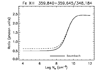
Figure 3.: Typical density-sensitive line intensity ratios computed for Fe XIII. Left panel: intensity ratios from a blend of two lines near 35.97 nm to another line, all within the $3s3p^{3}\,{}^{3}\!D^{o}-3s^{2}3p^{2}\,{}^{3}\!P$ multiplet. Right panel: a ratio of two lines within the $3s^{2}3p3d\,^{3}\!D^{o}-3s^{2}3p^{2}\,{}^{3}\!P$ multiplets. Dashed lines include radiative excitation, solid lines do not. Note that the ratios are sensitive in a density regime of interest [$n_{\rm e}\approx 10^{8}$ cm^-3]. Note that the wavelengths are in Å units not nm in the figure, and that atomic alignment is ignored in these calculations. The line marked “Baumbach” shows typical variations in electron density 1.005 to about 1.4 ${\rm R}_{\odot}$ as given by Baumbach in Allen (1973). fig:fe13dens

Other suitable ions (from the bright lines computed by Judge, 1998) include S-like Fe XI with an M1 line near 789.2 nm, B-like Mg VIII (3028 nm), C-like Si IX (3934 nm), and of course the red and green coronal lines (Cl-like Fe X and Al-like Fe XIV respectively). There are various pros/cons with the selection of lines. For example Fe XI 789.2 nm shows remarkable structure in eclipse images (Habbal et al., 2011), it lies in the near infrared so has low stray light and reasonable sensitivity to the Zeeman effect. It is formed at lower temperatures than Fe XIII and hence may be useful in cooler regions of the corona, say over coronal holes. As noted, this line is expected to have a small atomic alignment so that although the linear polarization will be small in 789.2 nm, so will the alignment corrections to the emission coefficients for Stokes-$I$ and $V$. It should therefore be considered as a prime target for future observations. A term diagram for Fe XI is shown in Figure fig:fe11_td. Cases can also be made for the other strong lines of various ions discussed by Judge (1998).

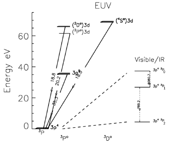
Figure 4.: Term diagram for S-like Fe XI. Unlike Si-like Fe XIII, the ground level has $J=2$, the 789.2 nm transition occurs between the upper $J=1$ level and the ground level. The $J=0\rightarrow J=1$ is at the anomalously large wavelength near 6082 nm because the Fe XI ion’s levels are close together as $jj$ coupling competes with $LS$ coupling (see Judge 1998). fig:fe11˙td

3 Tomographic-Inversions

Slicing through the volume containing magnetic-fields by observing lines of sight at different angles opens up the possibility of full 3D vector-field recovery. Some studies of vector tomography have been made by Kramar et al. (2006); Kramar and Inhester (2007). These are preliminary in that they explore either $I,V$ or $I,Q,U$, not the full Stokes vector. Further, just one theoretical emission-line was “inverted” so that the observed data contain limited information on the alignment $\sigma^{2}_{0}(\alpha_{0}J)$. They conclude however that

“We are confident that this data set is also sufficient to yield a realistic coronal magnetic-field model. This, however, has to be verified in future [numerical] experiments.”

Their method attempts to handle the existence of null spaces in the inversion by standard techniques of adding a “regularization” parameter. Thus far they have investigated the minimization of the functional

$$\ilabel{eq:functional}L({\bf B})=\mu({\bf I_{\rm OBS}-I_{\rm SIM}})\cdot({\bf I_{\rm OBS}-I_{\rm SIM}})+\int{\rm div^{2}}\,{\bf B}\,{\rm d}^{3}V$$ (14)

where the integral is over the coronal volume. Minimization of $L({\bf B})$ simply forces the selection of a 3D magnetic-field to minimize the differences between observed ${\bf I}_{\rm OBS}$ and computed ${\bf I}_{\rm SIM}$ intensities and polarized Stokes parameters, subject to the additional constraint depending on $\mu$. $\mu$ is a parameter that determines how much of the solution is determined by the data ($\mu$ large) and by the physically imposed divergence constraint ($\mu$ small). (Note that $\mu$ should include the estimates of the observed uncertainties for each component of the vector of observables too).

The divergence constraint alone means that the space of curl-free vector-fields is a null space: potential field components along the LOS are invisible to Stokes-$IV$. They speculate that by adding the force-free constraint into the regularization (as $\int|{\bf J\times B}|^{2}{\rm d}^{3}V$), this null space might be eliminated.

It should be remembered that such inversions rely on stereoscopic observations of coronal M1 lines (not currently possible) or on the assumption that the corona is a solidly rotating body, observed from the Earth over periods of at least a day.

If we combine our understanding from section sec:inversion with tomography, we see that with a general forward modeling code such as that written by Judge and Casini (2001), we can in principle invert a vector of observations including M1 lines with large and small alignment factors and selected E1 lines, to obtain the desired solutions for ${\bf B}({\bf r};t)$. Key to this effort will be the regular detection of the Stokes-$V$ parameters of M1 lines, something that has not yet been achieved owing to the small apertures of coronagraphs currently used. Unpublished work by Judge using the prototype CoMP instrument ($d=20$ cm) acquired in February 2012 gives an upper limit of 0.15 % for the maximum ratio of $V/I$ in 1079.8 nm. In 70 minute integrations and a low (20^′′) spatial resolution, Lin et al. (2004) achieved a sensitivity below 0.01%, leading to a Stokes-$V$ amplitude over an active region of about $0.0001I$, with a 0.46 m diameter coronagraph.

Clearly, bigger telescopes are needed at excellent sites for this kind of work to succeed. The COronal Solar Magnetism Observatory [COSMO] offers one possible solution.

4 Discussion

The tomographic-inversion scheme outlined above is the only way to invert formally data vectors to recover the coronal ${\bf B}({\bf r};t)$. The scheme relies on solar rotation and assuming the coronal structures are stationary over periods of a day or longer, or on the future availability of stereoscopic measurements both from earth and from a spacecraft (like the Solar TErrestrial RElations Observatory [STEREO]) at a significant elongation from the earth. The latter possibility has yet to be discussed at all and so is decades away. The former is naturally limited, but should be pursued once regular observations of the weak Stokes-$V$ signal are available. The CoMP instrument is a prototype for larger instruments which should achieve this goal (e.g., the Advanced Technology Solar Telescope [ATST], COSMO).

4.1 Local Analyses of Coronal Loops

It seems prudent also to relax our goal of reconstructing ${\bf B}({\bf r};t)$ via tomography and look to other ways that we might make progress in this area. One possibility is to assume that we can identify a single plasma loop in an M1 transition, as routinely done for EUV or X-ray data. In such a case the source vector [${\bf S}$] only has contributions predominantly from lines of sight that intersect the loop. Also let us assume that observations from another viewpoint (EUV data from STEREO for example) are available that fix the heliocentric coordinates of the plasma loop. This additional information enables us to diagnose magnetic-fields beyond what is possible from an isolated measurement of the Stokes profiles of a single point (Judge, 2007). However, as for EUV lines, no useful information outside the plasma loop volume is available. Nevertheless this should be pursued.

4.2 Direct Synthesis vs Observations

Another avenue to explore adding information to the data is to assume that we know more about the current-carrying structures that we are looking for. Thus, by building synthetic maps of M1 lines from models of the magnetic field and coronal plasma, and comparing them directly with observations, one can hope to extract meaningful information. It may be possible to argue that the data are inconsistent with a class of model (“i”), whereas another class (“ni”) is not inconsistent. Science advances often by identifying models of class (i), those of class (ni) being acceptable subject to further investigation. This will be a fruitful approach; already some initial comparisons reveal models of type (ni) (Rachmeler, 2012, in this volume) but as of yet we are not aware interesting cases in class (i). There are obvious cases where potential fields, extrapolated from the lower atmosphere fall into class (i), but this finding serves merely to show that some free magnetic energy appears necessary to describe coronal structures. This is something we have known for decades through other arguments (e.g. Gold and Hoyle, 1960).

These are early days though. The main issue with this approach is that

There are more things in heaven and earth, Horatio, than are dreamt of in your philosophy. – Hamlet

4.3 Closing thoughts on the “line-of-sight problem”

Consider the idea that in highly conducting plasma, one can trace magnetic-fields by looking at morphology of plasma loops. This was a motivation for the Transition Region and Coronal Explorer [TRACE] mission (hence its name) and it has yielded many such morphological analysis of “coronal magnetism”, including seismology (one nice example is that of Aschwanden et al., 1999). Apparently the LOS issues do not present special challenges in these analyses of coronal-intensity measurements. One might argue that these are seen against the dark solar disk (any EUV continuum emission from the low temperature photosphere/low chromosphere is very dark), whereas the M1 coronal lines must be observed above the limb against a dark background. But even in this case, isolated bright plasma loops organized into an active region offer no greater path lengths for integration than observations on the disk. Indeed, the discovery of MHD wave modes in the M1 Fe XIII 1074.7 nm line Tomczyk et al. (2007) indicates that, just as for EUV work, line of sight confusion is not an overwhelming problem.

We conclude that, as in all remotely sensed magnetic data, line of sight issues are important but not intractable. Often, using M1 lines we will be interested in the coronal magnetic-fields above active regions. These present themselves as bright isolated plasma loops in M1 coronal lines just as the EUV and X ray lines do (Bray et al., 1991), dominating the contributions to the Stokes vectors along the line of sight.

5 Conclusions

s:Conclusions

Scientific skepticism is healthy, and we certainly need to be skeptical of interpretations of all remotely sensed data of an object like the Sun. We have shown that the optically thin forbidden coronal lines suffer from the same kinds of interpretational problems as do other diagnostics of solar magnetism. We have suggested several ways to augment the data of isolated points in the corona - for which we have vast null spaces of unexplorable parameters - using tomography and traditional ideas concerning the smoothness and continuity of magnetic-fields in coronal structures, applied universally to EUV and X-ray intensity data.

It will be interesting to see how a full vector inversion including lines sensitive to thermodynamic parameters – both visible/IR M1 lines and EUV lines – will serve to further constrain tomographic-inversions. Certain schemes (especially “direct [matrix] inversions”) can be very fast, but these require linear Equations which is manifestly not the case (see the Equations above). It is, however, possible that the non-linearities introduced by the alignment into these equations can be treated to some degree by a formal (Newton-Raphson- style) linearization scheme. This seems promising given that we have lines with quite different alignment factors (1074.7 vs. 1079.8 or 798.2 nm) and thus different non-linear amplitudes, but this is an area that remains to be explored.

Several ways forward are reviewed while we await the arrival of high-sensitivity ($\lesssim 10^{-4}$) polarization data from telescopes (ATST, COSMO) needed for tomographic inversions that can recover the vector-field throughout volumes of the corona.

References

- Allen (1973) Allen, C.W.: 1973, Astrophysical Quantities, Athlone.
- Aschwanden et al. (1999) Aschwanden, M.J., Fletcher, L., Schrijver, C.J., Alexander, D.: 1999, Coronal Loop Oscillations Observed with the Transition Region and Coronal Explorer, Astrophys. J. 520, 880.
- Bray et al. (1991) Bray, R.J., Cram, L.E., Durrant, C.J., Loughhead, R.E.: 1991, Plasma Loops in the Solar Corona, Cambridge University Press.
- Casini and Judge (1999) Casini, R., Judge, P.G.: 1999, Spectral Lines for Polarization Measurements of The Coronal Magnetic Field. II. Consistent Theory of The Stokes Vector for Magnetic Dipole Transitions, Astrophys. J. 522, 524.
- Casini and Landi Degl’Innocenti (2008) Casini, R., Landi Degl’Innocenti, E.: 2008, in Plasma Polarization Spectroscopy, ed. Fujimoto, T. Iwamae, A., 247, Springer.
- Charvin (1965) Charvin, P.: 1965, Étude de la polarisation des raies interdites de la couronne solaire. Application au cas de la raie verte , Ann. Astrophys. 28, 877.
- Craig and Brown (1986) Craig, I. J.D., Brown, J.C.: 1986, Inverse problems in astronomy, Hilger
- Gold and Hoyle (1960) Gold, T., Hoyle, F.: 1960, On the origin of solar flares, Mon. Not. Roy. Astron. Soc. 120, 89.
- Habbal et al. (2011) Habbal, S.R., Druckmüller, M., Morgan, H., Ding, A., Johnson, J., Druckmüllerová, H., Daw, A., Arndt, M.B., Dietzel, M., Saken, J.: 2011, Thermodynamics of the Solar Corona and Evolution of the Solar Magnetic Field as Inferred from the Total Solar Eclipse Observations of 2010 July 11, Astrophys. J. 734, 120.
- Hale (1908) Hale, G.E.: 1908, On the Probable Existence of a Magnetic Field in Sun-Spots, Astrophys. J. 28, 315.
- Judge (1998) Judge, P.G.: 1998, Spectral Lines for Polarization Measurements of The Coronal Magnetic Field. I. Theoretical Intensities, Astrophys. J. 500, 1009.
- Judge (2007) Judge, P.G.: 2007, Spectral Lines for Polarization Measurements of the Coronal Magnetic Field. V. Information Content of Magnetic Dipole Lines, Astrophys. J. 662, 677.
- Judge and Casini (2001) Judge, P.G., Casini, R.: 2001, A Synthesis Code for Forbidden Coronal Lines, in Sigwarth, M., (ed.), Advanced Solar Polarimetry- Theory, Observation, and Instrumentation, CS-236, Astron. Soc. Pac. 503.
- Kramar and Inhester (2007) Kramar, M., Inhester, B.: 2007, Inversion of coronal Zeeman and Hanle observations to reconstruct the coronal magnetic field, Mem. S. A. It. 78, 120.
- Kramar et al. (2006) Kramar, M., Inhester, B., Solanki, S.K.: 2006, Vector tomography for the coronal magnetic field. I. Longitudinal Zeeman effect measurements, Astron. Astrophys. 456, 665.
- Lin et al. (2004) Lin, H., Kuhn, J.R., Coulter, R.: 2004, Coronal Magnetic Field Measurements, Astrophys. J. Lett. 613, L177.
- Parker (2007) Parker, E.N.: 2007, Conversations on Electric and Magnetic Fields in the Cosmos, Princeton.
- Rachmeler (2012) Rachmeler, L. et al.: 2012, this volume.
- Steiner (1994) Steiner, O.: 1994, Theoretical models of magnetic flux tubes: structure and dynamics, in J.T. Jefferies, D. Deeming, & D.R. Rabin (Eds.), Infrared Solar Physics, Proceedings IAU Symposium 154 (Tucson), Kluwer, Dordrecht, 407.
- Tomczyk et al. (2008) Tomczyk, S., Card, G.L., Darnell, T., Elmore, D.F., Lull, R., Nelson, P.G., Streander, K.V., Burkepile, J., Casini, R., Judge, P.G.: 2008, An Instrument to Measure Coronal Emission Line Polarization, Solar Phys. 247, 411.
- Tomczyk et al. (2007) Tomczyk, S., McIntosh, S.W., Keil, S.L., Judge, P.G., Schad, T., Seeley, D.H., Edmondson, J.: 2007, Alfvén Waves in the Solar Corona, Science 317, 1192.