Lattice Study of Radiative $J/\psi$ Decay to a Tensor Glueball

Abstract

The radiative decay of $J/\psi$ into a pure gauge tensor glueball is studied in the quenched lattice QCD formalism. With two anisotropic lattices, the multipole amplitudes $E_{1}(0)$, $M_{2}(0)$ and $E_{3}(0)$ are obtained to be $0.114(12)(6)$ GeV, $-0.011(5)(1)$ GeV, and $0.023(8)(1)$ GeV, respectively. The first error comes from the statistics, the $Q^{2}$ interpolation, and the continuum extrapolation, while the second is due to the uncertainty of the scale parameter $r_{0}^{-1}=410(20)$ MeV. Thus, the partial decay width $\Gamma(J/\psi\rightarrow\gamma G_{2^{++}})$ is estimated to be $1.01(22)(10)$ keV, which corresponds to a large branch ratio $1.1(2)(1)\times 10^{-2}$. The phenomenological implication of this result is also discussed.

Glueballs are exotic hadron states made up of gluons. Their existence is permitted by QCD but has not yet been finally confirmed by experiment. In contrast to the scalar glueball, whose possible candidate can be $f_{0}(1370)$, $f_{0}(1500)$, or $f_{0}(1710)$, the experimental evidence for the tensor glueball is more obscure. Quenched lattice QCD studies predict the tensor glueball mass to be in the range 2.2-2.4 GeV prd56 ; prd60 ; prd73 , which is also supported by a recent $2+1$ flavor full-QCD lattice simulation Gregory:2012 . In this mass region, Mark III Baltrusaitis:1986 and BES Bai:1996 have observed a narrow tensor meson $\xi(2230)$ [now as $f_{J}(2220)$ in PDGPDG2012 ] in the $J/\psi$ radiative decays with a large production rate, whose features favor the interpretation of a tensor glueball. However, it was not seen in the inclusive $\gamma$ spectrum Kopke:1989 by the Crystal Ball Collaboration and in $p\bar{p}$ annihilations to pseudoscalar pairs Barnes:1993 ; Hasan:1992 ; Hasan:1996 ; Bardin:1987 ; Sculli:1987 ; Evangelista:1997 ; Evangelista:1998 ; Buzzo:1997 . So, the existence of $\xi(2230)$ [$f_{J}(2220)$] needs confirmation by new experiments, especially by the BESIII experiment with the largest $J/\psi$ sample.

It is well known that the production of glueballs is favored in $J/\psi$ decays because of the gluon-rich environment. The radiative decay is of special importance, owing to its cleaner background. So, the production rate of the tensor glueball in the decay can be an important criterion for its identification. The decay has been studied only in a few theoretical works Li1981 ; Li:1987 ; Tenzo:1988 ; Melis:2004 . In these works, the tree-level perturbative QCD approach is employed. Under certain assumptions, the helicity amplitudes of the decay are related to the coupling of the two gluons to the tensor glueball. This coupling has been determined with the quenched lattice QCD prd73 ; Meyer2009 . Based on results of Refs. Li1981 ; Li:1987 ; Tenzo:1988 the branch ratio is estimated as $2\times 10^{-3}$ Li:2009 , but the theoretical uncertainties are not under control.

In fact, the decay can be investigated directly from the numerical lattice QCD studies dudek06 ; Gui:2013 , which provide first principles calculations from the QCD Lagrangian, especially in quenched lattice QCD. Quenched lattice QCD can be taken as a theory which only consists of heavy quarks and gluons. In this theory amplitudes of the decay do not have an absorptive part because of masses of states. Hence, the amplitudes can be directly calculated in the theory in Euclidian space. It should be noted that it is still a challenging task for the full-QCD lattice study of the decay because glueballs can be mixed with states of light quark pairs. Nevertheless, the study of the decay in quenched QCD will give important information about nonperturbative properties of glueballs.

At the lowest order of QED, the amplitude for the radiative decay $J/\psi\rightarrow\gamma G_{2^{++}}$ is given by

$$M_{r,r_{\gamma},r_{G}}=\epsilon_{\mu}^{*}(\vec{q},r_{\gamma})\langle G(\vec{p}_{f},r_{G})|j^{\mu}(0)|J/\psi(\vec{p}_{i},r)\rangle,$$ (1)

where $\vec{q}=\vec{p}_{i}-\vec{p}_{f}$ is the momentum of the real photon, and $r$, $r_{\gamma}$, and $r_{G}$ are the quantum numbers of the polarizations of $J/\psi$, the photon, and the tensor glueball, respectively. $\epsilon_{\mu}(\vec{q},r_{\gamma})$ is the polarization vector of the photon, and $j^{\mu}$ is the electromagnetic current operator. The hadronic matrix element appearing in the above equation can be obtained directly from a lattice QCD calculation of corresponding three-point functions. On the other hand, these matrix elements can be expressed (in Minkowski space-time) in terms of multipole form factors as follows:

$$\langle G(\vec{p}_{f},r_{G})|j^{\mu}(0)|J/\psi(\vec{p}_{i},r)\rangle=\alpha_{1}^{\mu}E_{1}(Q^{2})+\alpha_{2}^{\mu}M_{2}(Q^{2})$$

$$+\alpha_{3}^{\mu}E_{3}(Q^{2})+\alpha_{4}^{\mu}C_{1}(Q^{2})+\alpha_{5}^{\mu}C_{2}(Q^{2})$$ (2)

where $\alpha_{i}^{\mu}$ are Lorentz-covariant kinematic functions of $p_{i}$ and $p_{f}$ (and specific polarizations of the states), whose explicit expressions can be derived exactly Dudek2009 ; Yang:2012 , and $E_{1}(Q^{2})$, $M_{2}(Q^{2})$, $E_{3}(Q^{2})$, $C_{1}(Q^{2})$, and $C_{2}(Q^{2})$ are the form factors which depend only on $Q^{2}=-(p_{i}-p_{f})^{2}$. Since $C_{1}(Q^{2})$ and $C_{2}(Q^{2})$ vanish at $Q^{2}=0$, we focus on the extraction of the first three which are involved in the calculation of the decay width $\Gamma(J/\psi\rightarrow\gamma G_{2^{++}})$ as

$$\Gamma=\frac{4\alpha|\vec{p}_{\gamma}|}{27M_{J/\psi}^{2}}[|E_{1}(0)|^{2}+|M_{2}(0)|^{2}+|E_{3}(0)|^{2}],$$ (3)

where $\alpha$ is the fine structure constant, and $\vec{p}_{\gamma}$ is the photon momentum with $|\vec{p}_{\gamma}|=(M_{J/\psi}^{2}-M_{G}^{2})/(2M_{J/\psi})$.

We use the tadpole-improved gauge action prd56 to generate gauge configurations on anisotropic lattices with the aspect ratio $\xi=a_{s}/a_{t}=5$, where $a_{s}$ and $a_{t}$ are the spatial and temporal lattice spacings, respectively. Two lattices $L^{3}\times T=8^{3}\times 96(\beta=2.4)$ and $12^{3}\times 144(\beta=2.8)$ are applied to check the effect of the finite lattice spacings. The relevant input parameters are listed in Table 1, where $a_{s}$ values are determined from $r_{0}^{-1}=410(20)$ MeV. Since glueball relevant study needs quite a large statistics, the spatial extensions of both lattices are properly chosen to be $\sim 1.7$ fm according to the study of the finite volume effect study of Ref. prd73 , which is a compromise of the computational resource requirement and negligible finite volume effects both for glueballs prd73 and charmonia. In the practice, we generated 5000 configurations for each lattice. The charm quark propagators are calculated using the tadpole-improved clover action for anisotropic lattices chuan1 ; chuan2 with the bare charm quark masses set by the physical mass of $J/\psi$, $M_{J/\psi}=3.097$ GeV, through which the spectrum of the $1S$ and $1P$ charmonia are well reproduced Yang:2012 . In practice, disconnected diagrams due to the charm and quark-antiquark annihilation are expected to be unimportant according to the Okubo-Zweig-Iizuka rule and therefore are neglected in the calculation of relevant two-point and three-point functions.

Table 1: The input parameters for the calculation. Values for the coupling $\beta$, anisotropy $\xi$, the lattice size, and the number of measurements are listed. $a_{s}/r_{0}$ is determined by the static potential, and $a_{s}$ is estimated by $r_{0}^{-1}=410(20)$ MeV.

$\beta$	$\xi$	$a_{s}/r_{0}$	$a_{s}$(fm)	$La_{s}$(fm)	$L^{3}\times T$	$N_{\rm conf}$
2.4	5	0.461(4)	0.222(2)(11)	$\sim 1.78$	$8^{3}\times 96$	5000
2.8	5	0.288(2)	0.138(1)(7)	$\sim 1.66$	$12^{3}\times 144$	5000

The calculations in this Letter are performed in the rest frame of the tensor glueball. One of the key issues in our calculation is to construct optimal interpolating field operators which couple dominantly to the pure gauge tensor glueball. This is realized by applying completely the same scheme as that in the calculations of the glueball spectrum prd60 ; prd73 . On the cubic lattice, a tensor ($J=2$) state corresponds to the $E$ and $T_{2}$ irreducible representations of the lattice symmetry group $O$. So, we build the $E$ and $T_{2}$ operators from a set of prototype Wilson loops. By using different gauge-link smearing techniques, an operator set $\{\phi_{\alpha}^{(i)},\alpha=1,2,\ldots,24\}$ of 24 different gluonic operators is constructed for each component of the $T_{2}^{++}$ and $E^{++}$ representations, where the superscript $i$ labels the three components of $T_{2}$ and two components of $E$. Finally, for each component, an optimal operator $\Phi^{(i)}(t)=\sum v_{\alpha}\phi_{\alpha}^{(i)}(t)$ for the ground state tensor glueball is obtained with the combinational coefficients $v_{\alpha}$ determined by solving the generalized eigenvalue problem

$$\tilde{C}^{(i)}(t_{D}){\bf v}^{(R)}=e^{-t_{D}\tilde{m}(t_{D})}\tilde{C}^{(i)}(0){\bf v}^{(R)},$$ (4)

at $t_{D}=1$, where $\tilde{C}^{(i)}(t)$ is the correlation matrix of the operator set

$$\tilde{C}_{\alpha\beta}(t)=\frac{1}{N_{t}}\sum\limits_{\tau}\langle 0|{\phi}^{(i)}_{\alpha}(t+\tau){\phi}^{(i)}_{\beta}(\tau)|0\rangle.$$ (5)

In addition, the glueball two-point functions are normalized as

$$C^{i}(t) = \frac{1}{T}\sum\limits_{\tau}\langle\Phi^{(i)}(t+\tau)\Phi^{(i)\dagger}(\tau)\rangle$$ (6)

$$\approx \frac{|\langle 0|\Phi^{(i)}(0)|T_{i}\rangle|^{2}}{2M_{T}V_{3}}e^{-M_{T}t}\approx e^{-M_{T}t},$$

where $|T_{i}\rangle$ refers to $i$th component of the $T_{2}^{++}$ and $E^{++}$ glueball states. We are assured that $C^{i}(t)$ can be well described by a single exponential $C(t)=We^{-M_{T}t}$, with $W$ usually deviating from one by a few percents. It should be noted that the $SO(3)$ rotational symmetry is broken on the lattice with a finite lattice spacing, and consequently the masses of $T_{2}$ and $E$ glueballs are not necessarily the same, even though they converge to the same tensor glueball mass in the continuum limit when the rotational invariance is restored. However, with the two lattice spacings we used in this Letter, we observe that the difference of the two masses is not distinguishable within errors, which implies that the effects of the rotational symmetry breaking are not important. So, in the following, we neglect this symmetry breaking and assume that the five components of the $T_{2}$ and $E$ and that of the corresponding spin-two state can be connected by a normal transformation.

We calculate the three-point functions in the rest frame of the tensor glueball with $J/\psi$ moving with a definite momentum $\vec{p}_{f}=2\pi\vec{n}/La_{s}$, where $\vec{n}$ ranges from $(0,0,0)$ to $(2,2,2)$. In order to increase the statistics additionally, for each configuration, we calculate $T$ charm quark propagators $S_{F}(\vec{x},t;\vec{0},\tau)$ by setting a point source on each time slice $\tau$, which permits us to average over the temporal direction when calculating the three-point functions

$$\Gamma_{i,\mu,j}^{(3)}(\vec{q};t_{f},t) = \frac{1}{T}\sum\limits_{\tau=0}^{T-1}\sum\limits_{\vec{y}}e^{-i\vec{q}\cdot\vec{y}}\langle\Phi^{(i)}(t_{f}+\tau)$$ (7)

$$\times J_{\mu}(\vec{y},t+\tau)O_{V,j}(\vec{0},\tau)\rangle$$

$$= \sum\limits_{T,V,r}\frac{e^{-M_{T}(t_{f}-t)}e^{-E_{V}(\vec{q})t}}{2M_{T}V_{3}2E_{V}(\vec{q})}$$

$$\times\langle 0|\Phi^{(i)}(0)|T_{i}\rangle\langle T_{i}|J_{\mu}(0)|V(\vec{q},r)\rangle$$

$$\times\langle V(\vec{q},r)|O_{V,j}^{\dagger}(0)|0\rangle,$$

where $J_{\mu}(x)=\bar{c}(x)\gamma_{\mu}c(x)$ is the vector current operator, $O_{V,j}=\bar{c}\gamma_{j}c$ is the conventional interpolation field for $J/\psi$, and the summation in the last equality is over all the possible states with different polarizations. In the rest frame of the tensor glueball, the momentum of the initial $J/\psi$ is the same as that of the current operator, say, $\vec{p}_{V}=\vec{q}$. The vector current $J_{\mu}(x)$, which is conserved in the continuum limit, is no longer conserved on the lattice and requires a multiplicative renormalization. The renormalization constant of spatial components of the vector current is determined to be $Z_{V}^{(s)}=1.39(2)$ for $\beta=2.4$ and $Z_{V}^{(s)}=1.11(1)$ for $\beta=2.8$ Gui:2013 using a nonperturbative scheme dudek06 .

The matrix elements $\langle T_{i}|J_{\mu}(0)|V(\vec{q},r)\rangle$ can be extracted from the above three-point functions along with the two-point function of the glueball $C^{i}(t)$ and that of $J/\psi$ $\Gamma_{j}^{(2)}(\vec{q},t)$,

$$\Gamma_{j}^{(2)}(\vec{q},t)=\sum\limits_{\vec{x}}e^{-i\vec{q}\cdot\vec{x}}\langle 0|O_{V,j}(\vec{x},t)O_{V,j}^{\dagger}(\vec{0},0)|0\rangle,$$ (8)

which provide the information of $M_{T}$, $E_{V}(\vec{q})$, and the other two matrix elements. According to Eq. (6), one has approximately

$$\langle 0|\Phi^{(i)}(0)|T_{i}\rangle\approx\sqrt{2M_{T}V_{3}}.$$ (9)

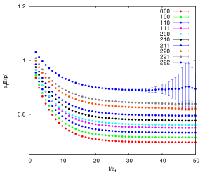
Figure 1: The effective energy plot for $J/\psi$ with different spatial momenta. From top to bottom are the plateaus for momentum modes, $\vec{p}=2\pi\vec{n}/L$, with $\vec{n}=(2,2,2)$, $(2,2,1)$, $(2,2,0)$, $(2,1,1)$, $(2,1,0)$, $(2,0,0)$, $(1,1,1)$, $(1,1,0)$, $(1,0,0)$, and $(0,0,0)$.

$M_{T}$ and $E_{V}(\vec{q})$ can be determined precisely from the two-point functions. Figure 1 shows the nice effective energy plateaus of $J/\psi$ for typical momentum modes at $\beta=2.4$. We also check the dispersion relation of $J/\psi$ and find the largest deviation of squared speed of light $c^{2}$ from one is less than 4%. The matrix elements $\langle V(\vec{q},r)|O_{V,j}^{\dagger}(0)|0\rangle$ are included implicitly in the three-point and two-point functions and can be canceled out by taking a ratio $R_{i,\mu,j}(\vec{q},t)$ for some specific $\{i,\mu,j\}$ combinations

$$R_{i,\mu,j}(\vec{q},t) = \Gamma^{(3)}_{i,\mu,j}(\vec{q},t_{f},t)\times$$

$$\frac{\sqrt{4V_{3}M_{T}E_{V}(\vec{q})}}{C^{i}(t_{f}-t)}\sqrt{\frac{\Gamma^{(2)}_{j}(\vec{q},t_{f}-t)}{\Gamma^{(2)}_{j}(\vec{q},t)\Gamma^{(2)}_{j}(\vec{q},t_{f})}},$$

which is expected to suppress the contamination from excited states of vector charmonia and should be insensitive to the variation of $t$ in a time window. As such, the desired matrix elements can be derived by the fit form

$$R_{i,\mu,j}(\vec{q},t)=\sum\limits_{r}\langle T_{i}|J_{\mu}(0)|V(\vec{q},r)\rangle\epsilon_{j}(\vec{q},r)+\delta f(t),$$ (11)

where $\vec{\epsilon}(\vec{q},r)$ is the polarization vector of $J/\psi$ and $\delta f(t)=ae^{-mt}$ accounts for the residual contamination from excited states.

In the data analysis, the 5000 configurations are divided into 100 bins and the average of 50 measurements in each bin is taken as an independent measurement. For the resultant 100 measurements, the one-eliminating jackknife method is used to perform the fit for the matrix elements ($M_{T}$ and $E_{V}$ determined from two-point functions are used as known parameters). Generally speaking, the time separations $t$ and $t_{f}-t$ should be kept large for the saturation of the ground state, but we have to fix $t_{f}-t=1$ because of the rapid damping of the glueball signal with respect to the noise. Fortunately this is justified to some extent by the optimal glueball operators, which couple almost exclusively to the ground state. The second step of the data analysis is to extract the form factors $E_{1}(Q^{2})$, $M_{2}(Q^{2})$, and $E_{3}(Q^{2})$ at different $Q^{2}=2E_{V}(\vec{q})M_{T}-M_{V}^{2}-M_{T}^{2}$ according to Eq. (Lattice Study of Radiative $J/\psi$ Decay to a Tensor Glueball). Since the matrix elements are measured from the same configuration ensemble, we carry out a correlated data fitting to get these three form factors simultaneously with a covariance matrix constructed from the jackknife ensemble described above. The symmetric combinations of the indices $\{i,\mu,j\}$ and the momentum $\vec{q}$ which gives the same $Q^{2}$ are averaged to increase the statistics. In order to get the form factor at $Q^{2}=0$, we carry out a correlated polynomial fit to the three form factors from $Q^{2}=-0.5$ to 2.7 ${\rm GeV}^{2}$,

$$F_{i}(Q^{2})=F_{i}(0)+a_{i}Q^{2}+b_{i}Q^{4},$$ (12)

where $F_{i}$ refers to $E_{1}$, $M_{2}$ or $E_{3}$. Figure 2 shows the results of $F_{i}(Q^{2})$ for $\beta=2.4$ (upper panel) and $\beta=2.8$ (lower panel), where the data points are the calculated values with jackknife errors, and the curves are the polynomial fits with jackknife error bands. The corresponding interpolated $F_{i}(0)$’s are listed in Table 2. Note that the renormalization constant $Z_{V}^{(s)}$ of the spatial components of the vector current is applied to the final numerical values. We also fit the form factors by functions either linear in $Q^{2}$ in the range $-0.5\,{\rm GeV^{2}}<Q^{2}<1.0\,{\rm GeV^{2}}$, or by adding a $Q^{6}$ term to Eq. (12) in the range $-0.5\,{\rm GeV^{2}}<Q^{2}<2.7\,{\rm GeV^{2}}$. The resultant $F_{i}(0)$’s are consistent with that of Eq. (12) within errors.

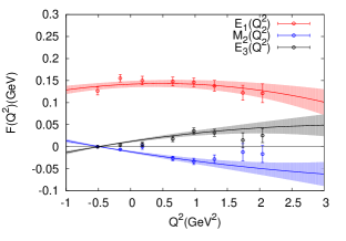
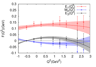
Figure 2: The extracted form factors $E_{1}(Q^{2})$, $M_{2}(Q^{2})$, and $E_{3}(Q^{2})$ in the physical units. The upper panel is for $\beta=2.4$ and the lower one for $\beta=2.8$. The curves with error bands show the polynomial fit with $F_{i}(Q^{2})=F_{i}(0)+a_{i}Q^{2}+b_{i}Q^{4}$.

The last step is the continuum extrapolation using the two lattice systems. After performing a linear extrapolation in $a_{s}^{2}$, the continuum limits of the three form factors are determined to be $E_{1}(0)=0.114(12)$ GeV, $M_{2}(0)=-0.011(5)$ GeV, and $E_{3}(0)=0.023(8)$ GeV, respectively. Considering the uncertainty of the scale parameter $r_{0}^{-1}=410(20)$ MeV, which also introduces $5\%$ error, the final result of the form factors is

$$E_{1}(0) = 0.114(12)(6)\,{\rm GeV}$$

$$M_{2}(0) = -0.011(5)(1)\,{\rm GeV}$$

$$E_{3}(0) = 0.023(8)(1)\,{\rm GeV}.$$ (13)

Note that there is a pattern $|E_{1}(0)|\gg|M_{2}(0)|\sim|E_{3}(0)|$; hence, the decay width is dominated by the value of $E_{1}(0)$. For the continuum value of the tensor glueball mass, we get $M_{G}=2.37(3)(12)$ GeV (the second error is due to the uncertainty of $r_{0}$), which is compatible with that in Ref. prd73 . Thus, according to Eq. (3), we finally get the decay width $\Gamma(J/\psi\rightarrow\gamma G_{2^{++}})=1.01(22)(10)$ keV. With the total width of $J/\psi$, $\Gamma_{\rm tot}=92.9(2.8)$ keV PDG2012 , the corresponding branching ratio is

$$\Gamma(J/\psi\rightarrow\gamma G_{2^{++}})/\Gamma_{\rm tot}=1.1(2)(1)\times 10^{-2}.$$ (14)

Table 2: The tensor glueball masses $M_{T}$ as well as the form factors $E_{1}(0)$, $M_{2}(0)$ and $E_{3}(0)$ for the two lattices with $\beta=2.4$ and 2.8. The last row gives the continuum extrapolation. The uncertainty of the scale parameter $r_{0}$ has not been incorporated yet.

$\beta$	$M_{T}$(GeV)	$E_{1}$ (GeV)	$M_{2}$ (GeV)	$E_{3}$ (GeV)
2.4	2.360(20)	0.142(07)	-0.012(2)	0.012(2)
2.8	2.367(25)	0.125(10)	-0.011(4)	0.019(6)
$\infty$	2.372(28)	0.114(12)	-0.011(5)	0.023(8)

The determined branching ratio is rather large. We admit that the calculation is carried out in the quenched approximation, whose systematical uncertainty cannot be estimated easily without unquenched calculations. A recent full-QCD lattice study of the mass spectrum of glueballs in Ref. Gregory:2012 indicates that there is no substantial correction of the masses of the scalar and tensor glueball. Based on this fact, if the form factors also show similar behavior as the masses, the unquenching effects might not change our result drastically. Of course, a full-QCD lattice calculation would be very much welcome.

In experiments, the narrow state $f_{J}(2220)$ observed by Mark III and BES in the $J/\psi$ decay was once interpreted as a candidate for the tensor glueball. But, the analysis of the processes $p\bar{p}\rightarrow\pi\pi(K\bar{K})$ yields no indication of the narrow $f_{J}(2220)$ and sets an upper bound for the branch ratios ${\rm Br}(f_{J}\rightarrow p\bar{p}){\rm Br}(f_{J}\rightarrow\pi\pi,K\bar{K})$ (see the review article Ref. Crede:2009 and the references therein). Combining this with the results of Mark III and BES, a lower bound for the branching ratio is obtained to be ${\rm Br}[J/\psi\rightarrow\gamma f_{J}(2220)]>2.5\times 10^{-3}$ PDG2012 , which seems compatible with our result. However, BESII with substantially more statistics does not find the evidence of a narrow structure around 2.2 GeV of the $\pi\pi$ invariant mass spectrum in the processes $J/\psi\rightarrow\gamma\pi\pi$ Ablikim06 , and BABAR does not observe it in $J/\psi\rightarrow\gamma(K^{+}K^{-},K_{S}K_{S})$ Sanchez:2010 . Recently, based on 225 million $J/\psi$ events, the BESIII Collaboration performs a partial wave analysis of $J/\psi\rightarrow\gamma\eta\eta$ and also finds no evident narrow peak for $f_{J}(2220)$ in the $\eta\eta$ mass spectrum Ablikim:2012 . So the existence of $f_{J}(2220)$ is still very weak. Another possibility also exists that the tensor glueball is a broad resonance and readily decays to light hadrons. Our result motivates a serious joint analysis of the radiative $J/\psi$ decay into tensor objects in $VV$, $PP$, $p\bar{p}$, and $4\pi$ final states (where $V$ and $P$ stand for vector and pseudoscalar mesons, respectively), among which $VV$ channels may be of special importance since they are kinematically favored in the decay of a tensor meson.

To summarize, we have carried out the first lattice study on the $E_{1}$, $M_{2}$, and $E_{3}$ multipole amplitudes for $J/\psi$ radiatively decaying into the pure gauge tensor glueball $G_{2^{++}}$ in the quenched approximation. With two different lattice spacings, the amplitudes are extrapolated to their continuum limits. The partial decay width and branch ratio for $J/\psi\rightarrow\gamma G_{2^{++}}$ are predicted to be $1.01(22)(10)$ keV and $1.1(2)(1)\times 10^{-2}$, respectively, which imply that the tensor glueball can be copiously produced in the $J/\psi$ radiative decays if it does exist. To date, the existence of $f_{J}(2220)$ needs confirmation and a broad tensor glueball is also possible. Hopefully, the BESIII data will be able to clarify the situation.

This work is supported in part by the National Science Foundation of China (NSFC) under Grants No.10835002, No.11075167, No.11021092, No.11275169, and No.10975076. Y. C. and C. L. also acknowledge the support of the NSFC and DFG (CRC110).

References

- (1) C.J. Morningstar and M. Peardon, Phys. Rev. D 56, 4043 (1997).
- (2) C.J. Morningstar and M. Peardon, Phys. Rev. D 60, 034509 (1999).
- (3) Y. Chen et al., Phys. Rev. D 73, 014516 (2006).
- (4) E. Gregory, A. Irving, B. Lucini, C. McNeile, A. Rago, C. Richards, and E. Rinaldi, J. High Energy Phys. 10 (2012) 170.
- (5) R.M. Baltrusaitis et al., Phys. Rev. Lett. 56, 107 (1986).
- (6) J.Z. Bai et al.(BES Collaboration), Phys. Rev. Lett. 76, 3502 (1996).
- (7) J. Beringer et al. (Particle Data Group), Phys. Rev. D 86, 010001 (2012).
- (8) L. Kopke and N. Wermes, Phys. Rep. 174, 67 (1989).
- (9) P.D. Barnes et al., Phys. Lett. B 309, 469 (1993).
- (10) A. Hasan et al., Nucl. Phys. B378, 3 (1992).
- (11) A. Hasan and D.V. Bugg, Phys. Lett. B 388, 376 (1996).
- (12) G. Bardin et al., Phys. Lett. B 195, 292 (1987).
- (13) J. Sculli, J.H. Christenson, G.A. Kreiter, P. Nemethy, and P. Yamin, Phys. Rev. Lett. 58, 1715 (1987).
- (14) C. Evangelista et al. (JETSET Collaboration), Phys. Rev. D 56, 3803 (1997).
- (15) C. Evangelista et al. (JETSET Collaboration), Phys. Rev. D 57, 5370(1998).
- (16) A. Buzzo et al. (JETSET Collaboration), Z. Phys. C 76, 475 (1997).
- (17) B.A. Li and Q.X. Shen, Phys. Lett. 126B, 125 (1983).
- (18) B.A. Li, Q.X. Shen, and K.-F. Liu, Phys. Rev. D 35, 1070 (1987).
- (19) K. Ishikawa, I. Tanaka, K.-F. Liu and B.A. Li, Phys. Rev. D 37, 3216 (1988).
- (20) M. Melis, F. Murgia, and J. Parisi, Phys. Rev. D 70, 034021 (2004).
- (21) H.B. Meyer, J. High Energy Phys. 01 (2009) 071.
- (22) G. Li, Y. Chen, B.-A. Li, and K.-F. Liu (unpublished).
- (23) L.-C. Gui, Y. Chen, G. Li, C. Liu, Y.-B. Liu, J.-P. Ma, Y.-B. Yang, and J.-B. Zhang, Phys. Rev. Lett. 110 021601 (2013).
- (24) J.J. Dudek, R.G. Edwards, and D.G. Richards, Phys. Rev. D 73, 074507 (2006).
- (25) Y.-B. Yang, Y. Chen, L.-C. Gui, C. Liu, Y.-B. Liu, Z. Liu, J.-P. Ma, and J.-B. Zhang, Phys. Rev. D 87, 014501 (2013).
- (26) J.J. Dudek, R.G. Edwards, and C.E. Thomas, Phys. Rev. D 79, 094504 (2009)
- (27) C. Liu, J. Zhang, Y. Chen, and J.P. Ma, Nucl. Phys. B624, 360 (2002).
- (28) S. Su, L. Liu, X. Li, and C. Liu, Int. J. Mod. Phys. A 21, 1015 (2006); Chin. Phys. Lett. 22, 2198 (2005).
- (29) V. Crede and C.A. Meyer, Prog. Part. Nucl. Phys. 63, 74 (2009).
- (30) M. Ablikim et al.(BES Collaboration), Phys. Lett. B 642, 441 (2006).
- (31) P. del Amo Sanchez et al. (BABAR Collaboration), Phys. Rev. Lett. 105, 172001 (2010).
- (32) M. Ablikim et al.(BES Collaboration), Phys. Rev. D 87, 092009 (2013).