Stability theory for difference approximations
of Euler Korteweg equations
and application to thin film flows

Abstract

We study the stability of various difference approximations of the Euler Korteweg equations. This system of evolution PDEs is a classical isentropic Euler system perturbed by a dispersive (third order) term. The Euler equations are discretized with a classical scheme (e.g. Roe, Rusanov or Lax Friedrichs scheme) whereas the dispersive term is discretized with centered finite differences. We first prove that a certain amount of numerical viscosity is needed for a difference scheme to be stable in the Von Neumann sense. Then we consider the entropy stability of difference approximations. For that purpose, we introduce an additional unknown, the gradient of a function of the density. The Euler Korteweg system is transformed into a hyperbolic system perturbed by a second order skew symmetric term. We prove entropy stability of Lax Friedrichs type schemes under a suitable Courant-Friedrichs-Levy condition. In addition, we propose a spatial discretization of the Euler Korteweg system seen as a Hamiltonian system of evolution PDEs. This spatial discretization preserves the Hamiltonian structure and thus is naturally entropy conservative. We validate our approach numerically on a shallow water system with surface tension which models thin films.

1 Introduction

This paper is motivated by the numerical simulation of the so-called Euler Korteweg system, which arises in the modeling of capillary fluids: these comprise liquid-vapor mixtures (for instance highly pressurized and hot water in nuclear reactors cooling system) [JTB], superfluids (Helium near absolute zero) [HAC], or even regular fluids at sufficiently small scales (think of ripples on shallow water or other thin films) [LG]. In one space dimension, the most general form of the Euler Korteweg system we consider is

$$\begin{array}[]{ll}{\displaystyle\partial_{t}\rho+\partial_{x}(\rho u)=0,}\\ {\displaystyle\partial_{t}(\rho u)+\partial_{x}\left(\rho u^{2}+P(\rho)\right)=\partial_{x}\left(\rho\kappa(\rho)\partial_{xx}\rho+(\rho\kappa^{\prime}(\rho)-\kappa(\rho))\frac{(\partial_{x}\rho)^{2}}{2}\right),}\end{array}$$ (1)

where $\rho$ denotes the fluid density, $u$ the fluid velocity$,P(\rho)$ the fluid pressure and $\kappa(\rho)>0$ the capillary coefficient. We assume that $P^{\prime}(\rho)>0$ for all $\rho>0$ so that the Euler system is always hyperbolic. In quantum hydrodynamics, the capillary coefficient is chosen so that $\rho\kappa(\rho)=constant$ [CDS] whereas for classical applications, like thin film flows, it is often chosen to be constant [BDK]. The Euler Korteweg system (1) falls in the class of abstract Hamiltonian systems of evolutions PDEs when it is written with variables $\rho,u$:

$${\displaystyle\partial_{t}U=\mathcal{J}\left({\rm E}\mathcal{H}[U]\right),}$$ (2)

with $U=(\rho,u)^{T}$, $\mathcal{J}=\partial_{x}{\rm J}$,

$${\displaystyle{\rm J}=\left(\begin{array}[]{cc}0&-1\\ -1&0\end{array}\right),\quad\mathcal{H}[U]=\frac{\rho u^{2}}{2}+F(\rho)+\kappa(\rho)\frac{(\partial_{x}\rho)^{2}}{2}=\frac{\rho u^{2}}{2}+\mathcal{E}(\rho,\partial_{x}\rho),}$$

and ${\rm E}$ denotes the Euler operator

$${\displaystyle{\rm E}\mathcal{H}[U]=\left(\begin{array}[]{c}{\displaystyle\frac{u^{2}}{2}+{\rm E}_{\rho}\mathcal{E}(\rho,\partial_{x}\rho)}\\ \rho u\end{array}\right),\>{\rm E}_{\rho}\mathcal{E}(\rho,\partial_{x}\rho)=F^{\prime}(\rho)+\kappa^{\prime}(\rho)\frac{(\partial_{x}\rho)^{2}}{2}-\partial_{x}(\kappa(\rho)\partial_{x}\rho).}$$

The pressure $P$ is related to $F$ through the relation $\rho F^{\prime}(\rho)-F(\rho)=P(\rho)$. Due to the invariance of the equations with respect to spatial and time translations, the system (2) admits, via Noether’s theorem, two additional conservation laws which are nothing but the conservation of momentum (the second equation of (1)) and the conservation of energy:

$${\displaystyle\partial_{t}\left(\frac{1}{2}\rho u^{2}+\mathcal{E}(\rho,\partial_{x}\rho)\right)+\partial_{x}\left(\frac{1}{2}\rho u^{3}+\rho u{\rm E}_{\rho}\mathcal{E}(\rho,\partial_{x}\rho)+\kappa(\rho)\partial_{x}(\rho u)\partial_{x}\rho\right)=0.}$$ (3)

As a consequence, if the system (1) is set on the real line or with periodic boundary conditions, the “entropy” $\mathcal{H}$ is conserved. Therefore, it is desirable from a numerical point of view that a difference approximation of (1) or (2) preserves the energy or, at least, dissipates energy. In the first case, the difference approximation is an “entropy conservative” scheme and in the later case, it is an “entropy stable” scheme.

There are two possible strategies to tackle this problem. The first one consists in considering (1) as a dispersive perturbation of the classical isentropic Euler equations. This is the point of view adopted e.g. in [LMR]. Here the authors construct fully discrete entropy conservative scheme for systems of conservation laws (hyperbolic or hyperbolic-elliptic) endowed with an entropy-entropy flux pair. These difference approximations are second and third order accurate and can in turn be used to construct a numerical method for the computation of weak solutions containing non- classical regularization-sensitive shock waves. In particular, the authors considered dissipative/dispersive regularizations that are linear in the entropy variables

$${\displaystyle\partial_{t}u(v^{\varepsilon})+\partial_{x}f(u(v^{\varepsilon}))=\varepsilon B_{2}\partial_{xx}v^{\varepsilon}+\varepsilon^{2}B_{3}\partial_{xxx}v^{\varepsilon},\quad 0<\varepsilon\ll 1}$$

with $B_{i}$ constant symmetric matrices, $B_{2}$ being positive definite. Thus the dispersive terms do not contribute in the energy equation:

$$\partial_{t}\int_{\mathcal{D}}U(u^{\varepsilon})\leq 0$$

where $\mathcal{D}=\mathbb{R}$ or $\mathcal{D}=\mathbb{R}/L\mathbb{Z}$ ($L>0$) and $U$ is the entropy associated to the system of conservation laws

$${\displaystyle\partial_{t}u+\partial_{x}f(u)=0.}$$

This situation contrasts with the one met in the Euler Korteweg system where the dispersive terms have a contribution in the energy balance

$${\displaystyle\partial_{t}\int_{\mathcal{D}}\frac{1}{2}\rho u^{2}+F(\rho)+\kappa(\rho)\frac{(\partial_{x}\rho)^{2}}{2}\,dx=0.}$$

As a consequence, an entropy conservative or entropy stable scheme for the isentropic Euler equations coupled with a centered approximation of dispersive terms may not provide an entropy conservative nor entropy stable scheme for the Euler Korteweg system. This issue was considered in [CL] where Euler Korteweg equations are written in lagrangian coordinates of mass: by introducing an extended formulation of the system, the authors derived a family of high order and entropy conservative semi-discrete schemes. With these high order approximations schemes in hand, the authors then computed kinetic relations for Van der Waals fluids. In [HR], an alternative reduction of order of the Euler Korteweg system in lagrangian coordinates of mass is introduced to derive a semi-discrete entropy conservative scheme based on local Galerkin discontinuous methods. Though, the lagrangian coordinates of mass can not be used in dimension $d$ with $d\geq 2$ and one has to consider an alternative extended formulation in Eulerian coordinates: this latter point of view will be expanded here, based on the extended formulation found in [BDD, BDDd].

In section 2, we consider the stability of various difference approximations of Euler Korteweg equations in the Von Neumann sense. We shall prove that even at that linear level, the Godunov scheme (explicit and implicit in time) is always unstable. In this direction, we checked the stability of Lax Friedrichs type schemes: we show that it is stable in the Von Neumann sense under a suitable Courant-Friedrichs-Levy (CFL) condition for explicit forward Euler (resp. Runge Kutta) time discretization for first order (resp. second order) difference schemes. This analysis provides necessary conditions of stability for the simulations of the fully nonlinear system. Finally we show that the backward Euler and Crank Nicolson time discretization is always stable for Lax Friedrichs type schemes.

In section 3, we move to the entropy (nonlinear) stability problem. It is a hard problem to obtain directly entropy stability from nonlinear difference approximation of Euler Korteweg equations since discrete integration by parts and time discretization do not commute. Here, we introduce an additional variable $w=\sqrt{\kappa(\rho)}\partial_{x}\rho/\sqrt{\rho}$ and derive a conservation law for $w$. In this new formulation, the capillary term appears as an anti dissipative term in the system for $(u,w)$ and one can prove the well posedness of the Euler Korteweg system [BDD]. Moreover, the derivation of the energy estimate follows the same line as a classical energy estimate in the isentropic Euler equations. In that setting, we show that difference approximations made of a Lax Friedrichs type (entropy stable) scheme for the hyperbolic part and centered difference for the anti-diffusive part are entropy stable under a suitable CFL condition for explicit forward Euler time discretization and always stable for implicit backward Euler time discretization. We also introduce an alternative method to obtain directly entropy conservative scheme. For that purpose, we write the Euler Korteweg system as a Hamiltonian system of PDEs: by discretizing directly the Hamiltonian, we obtain a semi discrete scheme that is also Hamiltonian and entropy is trivially preserved. Then, one is left with the problem of time discretization: the explicit forward Euler is always unstable and one has to consider implicit time discretization to obtain an entropy stable scheme

Finally, in section 4, we carry out numerical simulations of shallow water equations with surface tension which is a particular case of the Euler Korteweg equations. We first consider thin film flow over a flat bottom and neglect source terms so as to compare entropy stability of difference approximations for shallow water in original form and for its new formulation counterpart. The numerical simulations clearly show that the discretization of the extended formulation of shallow water equations has better entropy stability properties. Then, we consider the difference approximation of the shallow water equations written as a Hamiltonian system of evolution PDEs. The numerical simulation of this Hamiltonian system shows that the dynamical behavior is completely changed in comparison to entropy stable schemes. Indeed, this Hamiltonian difference approximation has no numerical viscosity, so that one can observe the formation of so called “dispersive shock waves” [E, EGK, EGS]. Here, the classic hyperbolic shocks are regularized by dispersive effects and an oscillatory zone appear and grows with time. We conclude this section with numerical simulation of a Liu Gollub experiment [LG] modeled by a consistent shallow water model with source term derived in [NV]. The numerical simulation show very good agreement with the experiments in [LG].

2 Von Neumann stability of difference schemes

In this section, we study the Von Neumann stability of various difference approximations. We consider two classes of spatial discretizations, namely Godunov and Lax Friedrichs schemes for the first order part of the equations whereas the dispersive term is discretized with classical centered difference approximations. We also consider second order accurate schemes, namely MUSCL scheme with a Lax Friedrichs type flux for spatial discretization together with Runge Kutta (second order accurate) or Crank Nicolson time discretization.

2.1 Stability of first order accurate schemes

In this section, we prove that Godunov space discretization are always unstable whereas Lax Friedrichs type scheme are stable under CFL conditions.

2.1.1 Formulation of the stability problem

In order to study the Von Neumann stability, we first linearize the Euler Korteweg equations about a constant state $(\rho,q)=(\bar{\rho},\bar{\rho}\bar{u})$:

$$\partial_{t}v+A\partial_{x}v=B\partial_{xxx}v,\quad A=\left(\begin{array}[]{cc}0&1\\ \bar{c}^{2}-\bar{u}^{2}&2\bar{u}\end{array}\right),\quad B=\left(\begin{array}[]{cc}0&0\\ \bar{\sigma}&0\end{array}\right)$$ (4)

with $v=(\rho,q)^{T}$, $\bar{\sigma}=\bar{\rho}\kappa(\bar{\rho})$ and $\bar{c}=\sqrt{P^{\prime}(\bar{\rho})}$. We discretize space and denote $v_{j}(t)$ the approximate value of $v(t,j\delta x),j\in\mathbb{Z}$ and $\delta x>0$. We also introduce the Fourier transform of a sequence $v\in l^{2}(\mathbb{Z})$:

$$\hat{v}(\theta)=\sum_{k\in\mathbb{Z}}e^{ik\theta}v_{k},\qquad\|v\|_{l^{2}(\mathbb{Z})}=\|\hat{v}\|_{L^{2}_{per}(0,2\pi)}.$$

In what follows, we consider Godunov, Lax Friedrichs and Rusanov discretization of the first order part whereas the capillary term is discretized with centered difference. These schemes have the common formulation

$$\displaystyle\frac{dv_{j}}{dt}+\frac{A}{2\delta x}\left(v_{j+1}-v_{j-1}\right) = \frac{Q}{2\delta t}\left(v_{j+1}-2v_{j}+v_{j-1}\right)$$ (5)

$$+\frac{B}{2\delta x^{3}}\left(v_{j+2}-2v_{j+1}+2v_{j-1}-v_{j-2}\right),$$

with $Q={\rm Id}$ for Lax Friedrichs scheme, $Q=(1/2){\rm Id}$ for the modified Lax Friedrichs scheme, $Q=(\delta t/\delta x)\rho(A)$ for Rusanov ($\rho(A)=\max\{|\lambda|,\lambda\in{\rm Sp}(A)\}$), $Q=(\delta t/\delta x)|A|$ for Godunov scheme with

$$|A|=\frac{1}{2\bar{c}}\left(\begin{array}[]{cc}\displaystyle|\bar{u}-\bar{c}|(\bar{u}+\bar{c})-|\bar{u}+\bar{c}|(\bar{u}-\bar{c})&|\bar{u}+\bar{c}|-|\bar{u}-\bar{c}|,\\ \displaystyle(\bar{c}^{2}-\bar{u}^{2})\left(|\bar{u}+\bar{c}|-|\bar{u}-\bar{c}|\right)&|\bar{u}+\bar{c}|(\bar{u}+\bar{c})-|\bar{u}-\bar{c}|(\bar{u}-\bar{c})\end{array}\right)$$

We apply the Fourier Transform to (5): $\hat{v}$ satisfies the differential system:

$$\frac{d\hat{v}}{dt}=i\frac{2\sin(\theta/2)\cos(\theta/2)}{\delta x}A\hat{v}-\frac{\delta x^{2}}{2\delta t}\left(\frac{2\sin(\theta/2)}{\delta x}\right)^{2}Q\hat{v}+i\cos(\theta/2)\left(\frac{2\sin(\theta/2)}{\delta x}\right)^{3}B\hat{v}.$$

We introduce the Fourier variable $\xi=2\sin(\theta/2)/\delta x$ so that $\hat{v}$ satisfies

$$\frac{d\hat{v}}{dt}=\left(\sqrt{1-\frac{(\xi\delta x)^{2}}{4}}\left(i\xi A+i\xi^{3}B\right)-\xi^{2}\left(\frac{\delta x^{2}}{2\delta t}\right)Q\right)\hat{v}:=i\xi M(\xi,\delta x)\hat{v},$$ (6)

with matrix $M(\xi,\delta x)$ defined as

$$M(\xi,\delta x)=\zeta\left(A+\xi^{2}B\right)+i\xi\frac{\delta x^{2}}{2\delta t}Q,\quad\zeta=\sqrt{1-\frac{(\xi\delta x)^{2}}{4}}.$$

In what follows, we consider the stability of the forward Euler, backward Euler and $\Theta$ scheme time discretization of (6): it reads, respectively, for all $n\geq 0$

$$\begin{array}[]{lll}\displaystyle\hat{v}^{n+1}=\left({\rm Id}+i\xi\delta tM(\xi,\delta x)\right)\hat{v}^{n},\qquad(FE),\\ \displaystyle\hat{v}^{n+1}=\left({\rm Id}-i\xi\delta tM(\xi,\delta x)\right)^{-1}\hat{v}^{n},\qquad(BE),\\ \displaystyle\hat{v}^{n+1}=\left({\rm Id}-i\Theta\xi\delta tM(\xi,\delta x)\right)^{-1}\left({\rm Id}+i(1-\Theta)\xi\delta tM(\xi,\delta x)\right)\hat{v}^{n},\qquad(\Theta\,S).\end{array}$$

We denote $\Lambda_{\pm}(\xi,\delta x)=R_{\pm}(\xi,\delta x)+iI_{\pm}(\xi,\delta x)$ the eigenvalues of $M(\xi,\delta x)$. The proof of the following proposition is straightforward and left to the reader:

Proposition 1.

A necessary condition for the (FE), (BE) and $(\Theta S)$ time discretizations to be stable is

$$\xi I_{\pm}(\xi,\delta x)\geq 0,\quad\forall\xi\in\left[-\frac{2}{\delta x},\,\frac{2}{\delta x}\right].$$ (7)

This condition is sufficient for (BE) scheme and $(\Theta S)$ scheme for all $\Theta\geq 1/2$. The $(\Theta S)$ and (FE) scheme (which corresponds to the $0S$ scheme) are stable under the condition:

$$\delta t\leq\frac{2\xi\,I_{\pm}(\xi,\delta x)}{(1-2\Theta)\xi^{2}(R_{\pm}^{2}(\xi,\delta x)+I_{\pm}^{2}(\xi,\delta x))},\quad\forall\xi\in\left[-\frac{2}{\delta x},\,\frac{2}{\delta x}\right].$$ (8)

Remark. Note that for $\delta x\to 0$, the condition $\xi I_{\pm}(\xi,0)\geq 0$ for all $\xi\in\mathbb{R}$ is nothing but the dissipativity of the operator $Mv:=-A\partial_{x}v+(\delta x^{2}\,Q/(2\delta t))\partial_{xx}v+B\partial_{xxx}v$.

2.1.2 Stability/Instability of first order schemes

We are now in a position to prove the instability of Godunov/Roe type scheme. In this section, we will have to consider various Courant-Friedrichs-Lewy conditions (denoted CFL condition): we introduce $\lambda_{j}=\delta t/\delta x^{j}$ for $j=1,2,3$.

Proposition 2.

Assume $Q=\lambda_{1}|A|$ (Roe/Godunov scheme), then for $\xi\delta x>0$ fixed and as $|\xi|\to\infty$, one has

$$\xi I_{\pm}(\xi,\delta x)\sim\pm\xi|\xi|\left(\sqrt{\bar{\sigma}^{2}\zeta^{4}+2\bar{\sigma}\zeta\sqrt{1-\zeta^{2}}|A|_{12}}-\bar{\sigma}\zeta^{2}\right).$$

As a consequence, the Godunov/Roe space discretization is always unstable regardless to the (FE), (BE) and $(\Theta S)$ time discretizations.

Remark The previous proposition also proves that the PDE

$$\partial_{t}v+A\partial_{x}v=\frac{\delta x}{2}|A|\partial_{xx}v+B\partial_{xxx}v$$

is ill-posed in $L^{2}(\mathbb{R})$, it is therefore hopeless to find a stable scheme for Godunov/Roe spatial discretizations. This is the main difference between the scalar case where the numerical viscosity induces dissipation and the system case where numerical viscosity interacts with surface tension and leads to instability/ill-posedness.

Proof.

Set $\displaystyle\zeta=\sqrt{1-\frac{\xi^{2}\delta x^{2}}{4}}$ and $q_{ij}=\delta x|A|_{ij}/2$, then the eigenvalues $\Lambda_{\pm}(\delta x,\xi)$ of $M(\xi,\delta x)$ are written as

$$\displaystyle\Lambda_{\pm}(\xi,\delta x) = \zeta\bar{u}+i\xi\frac{q_{11}+q_{22}}{2}\pm\sqrt{\Delta},$$

$$\displaystyle\Delta = \zeta^{2}(\bar{c}^{2}+\bar{\sigma}\xi^{2})-\xi^{2}\left(\frac{(q_{11}-q_{22})^{2}}{4}+q_{12}q_{21}\right)$$

$$+i\xi\zeta\left(\bar{u}(q_{22}-q_{11})+q_{21}+q_{12}(\bar{c}^{2}-\bar{u}^{2})+\bar{\sigma}q_{12}\xi^{2}\right).$$

As $\delta x\to 0$, $\Lambda_{\pm}(\xi,\delta x)$ expands as

$$\Lambda_{\pm}(\xi,\delta x)=\pm\sqrt{\bar{\sigma}\zeta}\sqrt{\zeta+i\sqrt{1-\zeta^{2}}|A|_{12}}|\xi|+O(1).$$

Then, one finds

$$\xi I_{\pm}(\xi,\delta x)=\pm\xi|\xi|\left(\sqrt{\bar{\sigma}^{2}\zeta^{4}+2\bar{\sigma}\zeta\sqrt{1-\zeta^{2}}|A|_{12}}-\bar{\sigma}\zeta^{2}\right)+O(\xi).$$

This completes the proof of the instability of Godunov/Roe space discretization ∎

Let us now consider the stability of Lax Friedrichs type schemes. We will assume that $Q=\lambda_{1}q\,{\rm Id}$ with $q=1/\lambda_{1}$ for the Lax Friedrichs scheme, $q=1/(2\lambda_{1})$ for the modified one and $q=\rho(A)$ for the Rusanov scheme. It is an easy computation to show that

$$\Lambda_{\pm}(\xi,\delta x)=\zeta(\bar{u}\pm\sqrt{\bar{c}^{2}+\bar{\sigma}\xi^{2}})+i\frac{\xi\delta x}{2}q,\quad\zeta=\sqrt{1-\frac{\xi^{2}\delta x^{2}}{4}}.$$

Proposition 3.

Assume $Q=\displaystyle\lambda_{1}q{\rm Id}$, then the (BE) and $(\Theta S)$ time discretization are unconditionally stable for all $\Theta\geq 1/2$. If $\Theta<1/2$, the $(\Theta S)$ scheme is stable under the condition.

$$\left((1-s)\left(\bar{u}\pm\sqrt{\bar{c}^{2}+\frac{4\bar{\sigma}s}{\delta x^{2}}}\right)^{2}+sq^{2}\right)\frac{\lambda_{1}}{q}\leq\frac{2}{1-2\Theta},\quad\forall s\in\left[0,1\right].$$

One can derive a, simpler, sufficient condition of stability: indeed, it is easily seen that the above condition is satisfied if

$$\max\left(\left(|\bar{u}|+\sqrt{\bar{c}^{2}+\frac{4\bar{\sigma}}{\delta x^{2}}}\right)^{2},\>q^{2}\right)\frac{\lambda_{1}}{q}\leq\frac{2}{1-2\Theta}$$

Corollary 4.

The Lax Friedrichs scheme $q=1/\lambda_{1}$ is stable if

$$(|\bar{u}|+|\bar{c}|)\lambda_{1}+2\sqrt{\bar{\sigma}}\lambda_{2}\leq\sqrt{\frac{2}{(1-2\Theta)}}.$$

The modified Lax Friedrichs scheme $q=1/(2\lambda_{1})$ is stable if

$$(|\bar{u}|+|\bar{c}|)\lambda_{1}+2\sqrt{\bar{\sigma}}\lambda_{2}\leq\sqrt{\frac{1}{(1-2\Theta)}}.$$

The Rusanov scheme $q=\rho(A)$ is stable if

$$\max\left(\left(|\bar{u}|\delta x+\sqrt{\bar{c}^{2}\delta x^{2}+4\bar{\sigma}}\right)^{2}\lambda_{3},\rho(A)^{2}\lambda_{1}\right)\leq\frac{2\rho(A)}{1-2\Theta}.$$

One can show formally that the (CFL) condition $\delta t=O(\delta x^{2})$ for Lax Friedrichs scheme is sharp. The wave speeds of (4) are $s(\xi)=\bar{u}\pm\sqrt{\bar{c}^{2}+\bar{\sigma}\xi^{2}}$. Hence, in the limit $|\xi|\to\infty$, one has $s(\xi)\leq\bar{C}|\xi|$. Heuristically, it is necessary for a numerical scheme to be stable that the domain of dependence of the numerical solution contains the domain of dependence of the exact solution. This condition reads $s(\xi)\,\delta t/\delta x<1$. On a spatial grid with stepsize $\delta x$, one has $s(\xi)\leq\bar{C}/\delta x$ since the largest wavenumber is $O(1/\delta x)$. As a consequence, one obtains a (formal) CFL condition $\bar{C}\delta t/\delta x^{2}<1$ which is precisely the CFL condition for the Lax Friedrichs scheme. The (CFL) found for the Rusanov scheme shows that this condition is not sufficient.

Note that if $\Theta=1/2$ (Crank Nicolson scheme), one can choose $Q=0$ and consequently a spatial centered scheme. This corresponds to the numerical schemes used for the practical simulation of thin film flows down an inclined plane in the presence of surface tension [KRSV].

2.2 Second order accurate schemes

Hereafter, we consider second order accurate schemes. For the time discretization, we consider the (second order) Runge Kutta and the Crank Nicolson methods. We discretize (4) in space by using a MUSCL scheme [Col, VL] for the first order differential operator without nonlinear monotony correction of the slope (it does not operate in the smooth monotone area of the solution), and centered approximation of third order differential terms:

$$\displaystyle\frac{dv_{j}}{dt} = \frac{A\left(v_{j+2}-6v_{j+1}+6v_{j-1}-v_{j-2}\right)}{8\delta x}$$ (9)

$$+ \frac{Q}{2\delta t}\frac{\left(-v_{j+2}+4v_{j+1}-6v_{j}+4v_{j-1}-v_{j-2}\right)}{8}$$

$$+ \frac{B}{2\delta x^{3}}\left(v_{j+2}-2v_{j+1}+2v_{j-1}-v_{j-2}\right)$$

with $j\in\mathbb{Z}$. In Fourier variables, the equation (9) now reads

$$\frac{d\hat{v}}{dt}=i\xi\mathcal{M}(\xi,\delta x)\hat{v},\quad\mathcal{M}(\xi,\delta x)=\zeta\left((1+\frac{\xi^{2}\delta x^{2}}{4})A+\xi^{2}B\right)+i\xi\left(\frac{\xi^{2}\delta x^{4}}{16\delta t}Q\right).$$ (10)

In what follows, we only consider second order accurate time discretization. First, the second order accurate Runge Kutta time discretization reads

$$\hat{v}^{n+1}=\left({\rm Id}+i\xi\delta t\mathcal{M}(\xi,\delta x)-\frac{\xi^{2}\delta t^{2}}{2}\mathcal{M}(\xi,\delta x)^{2}\right)\hat{v}^{n}.$$ (11)

Assume $Q=\lambda_{1}q{\rm Id}$: the eigenvalues $\Lambda_{\pm}(\xi,\delta x)$ are given by

$$\Lambda_{\pm}(\xi,\delta x)=\zeta(2-\zeta^{2})\left(\bar{u}\pm\sqrt{\bar{c}^{2}+\frac{\bar{\sigma}}{2-\zeta^{2}}\xi^{2}}\right)+iq\frac{\xi\delta x}{4}(1-\zeta^{2}).$$

Then, the Runge Kutta scheme is stable if and only if

$${\displaystyle{\left|1+i\xi\delta t\Lambda_{\pm}(\xi,\delta x)-\frac{\xi^{2}\delta t^{2}}{2}\Lambda_{\pm}(\xi,\delta x)^{2}\right|\leq 1}}$$

The proof of the following proposition is straightforward

Proposition 5.

The second order accurate scheme with MUSCL type discretization in space and Runge Kutta time discretization is stable if and only if $0<q\lambda_{1}\leq 2$ and, for all $s=1-\zeta^{2}\in[0,1]$

$$\left(|\bar{u}|+\sqrt{\bar{c}^{2}+\frac{s}{1+s}\frac{4\bar{\sigma}}{\delta x^{2}}}\right)^{2}\lambda_{1}^{2}\leq\frac{q\lambda_{1}s(2-q\lambda_{1}s^{2})+2\sqrt{2q\lambda_{1}-(q\lambda_{1})^{2}s^{2}}}{4(1+s)(1-s)}$$ (12)

From this proposition, we deduce the following simplified (CFL) conditions:

Corollary 6.

The classical Lax Friedrichs scheme with MUSCL space and Runge Kutta time discretization is stable in the Von Neumann sense if

$${\lambda_{1}{\displaystyle\left(\bar{u}+\sqrt{\bar{c}^{2}+\frac{2\bar{\sigma}}{\delta x^{2}}}\right)\leq 1}}$$

When $\delta x$ is sufficiently small one finds the following condition:

$$\frac{\delta t}{\delta x{}^{\frac{7}{3}}}\leq\left(\frac{\sqrt{\left(\bar{u}+\bar{c}\right)}}{\bar{\sigma}}\right)^{\frac{2}{3}}\frac{7^{\frac{7}{6}}\sqrt{3}}{24}+O\left(\delta x\right)+O\left(\sqrt{\lambda_{1}}\right)$$

for the Rusanov scheme with MUSCL space discretization

Note that we get an improved (CFL) condition $\delta t=O(\delta x^{7/3})$ for the Rusanov scheme that is almost sharp in comparison to first order accurate schemes. We finish this section by checking the stability of the Crank Nicolson scheme ($\Theta$-scheme with $\Theta=1/2$).

Proposition 7.

The difference approximation with Crank Nicolson type time discretization and second order accurate in space (MUSCL with Lax Friedrichs fluxes) is stable for all $Q\geq 0$.

Proof.

In Fourier variables, the Crank Nicolson scheme for 9 reads

$${\displaystyle{\hat{v}^{n+1}=\left(1-\frac{i\xi\delta t}{2}\mathcal{M}(\xi,\delta x)\right)^{-1}\left(1+\frac{i\xi\delta t}{2}\mathcal{M}(\xi,\delta x)\right)\hat{v}^{n}.}}$$

It is stable if and only if

$$\left|1+\frac{i\xi\delta t}{2}\Lambda_{\pm}(\xi,\delta x)\right|\leq\left|1-\frac{i\xi\delta t}{2}\Lambda_{\pm}(\xi,\delta x)\right|.$$

It is easily seen that this condition is equivalent to $\Im(\xi\Lambda_{\pm}(\xi,\delta x))\geq 0$ which obviously holds true for any $q\geq 0$, and this concludes the proof of the proposition.∎

3 Entropy stability of difference approximations

In this section, we study the entropy stability of difference approximations for Euler Korteweg equations (1). In order to simplify the discussion, we assume that (1) is set on a bounded interval $[0,L]$ with periodic boundary conditions. Recall that $(\rho,u)$ solution of (1) satisfies the energy estimate

$${\displaystyle\partial_{t}\int_{\mathcal{D}}\rho\frac{u^{2}}{2}+F(\rho)+\kappa(\rho)\frac{(\partial_{x}\rho)^{2}}{2}dx=0,}$$ (13)

with $\mathcal{D}=\mathbb{R}/L\mathbb{Z}$. The surface tension plays a significant role in the energy estimate and the previous section illustrates that it is a non trivial task to obtain a numerical scheme which conserves or, at least, dissipates the energy, even at the linearized level.

In this section, we introduce a new unknown $w=\sqrt{\kappa(\rho)}\partial_{x}\rho/\sqrt{\rho}$ and derive an evolution equation for $w$. The system of evolution PDEs for $(\rho,\rho u,\rho w)$ is made of a first order hyperbolic part perturbed by a second order anti dissipative term. This latter term is discretized by centered finite differences. We show that any entropy dissipative schemes for the hyperbolic part (in the sense defined by Tadmor in [T]), provides an entropy dissipative scheme for the “augmented” Euler Korteweg system.

In addition, we introduce an alternative discretization of (1) by writing this system as a Hamiltonian system of PDEs. By discretizing the Hamiltonian and writing the associated Hamiltonian system of ODEs, we find a consistent semi discrete scheme that is naturally entropy conservative.

3.1 Extended formulation of the Euler-Korteweg system

We start from the system (1). Following [BDD], we introduce $w=\sqrt{\kappa(\rho)}\partial_{x}\rho/\sqrt{\rho}$. One finds:

$${\displaystyle\partial_{t}\rho+\partial_{x}(\rho u)} = 0,$$ (14)

$${\displaystyle\partial_{t}(\rho u)+\partial_{x}(\rho u^{2}+P(\rho))} = \partial_{x}\left(\mu(\rho)\partial_{x}w\right),$$ (15)

$${\displaystyle\partial_{t}(\rho w)+\partial_{x}(\rho u\,w)} = -\partial_{x}\left(\mu(\rho)\partial_{x}u\right),$$ (16)

with $\mu(\rho)=\rho^{3/2}\sqrt{\kappa(\rho)}$. The equation (16) is derived by multiplying (14) by $\sqrt{\rho\kappa(\rho)}$ and deriving the resulting equation with respect to $x$. Let us set $v=(\rho,\rho u,\rho w)^{T}$ and $f(v)=(\rho u,\rho u^{2}+P(\rho),\rho uw)^{T}$: the system (14-16) now reads

$${\displaystyle\partial_{t}v+\partial_{x}f(v)=\partial_{x}\left(B(\rho)\partial_{x}\,z\right),}$$ (17)

where $B(\rho)$ denotes the skew-symmetric matrix

$${\displaystyle B(\rho)=\left(\begin{array}[]{ccc}0&0&0\\ 0&0&\mu(\rho)\\ 0&-\mu(\rho)&0\end{array}\right),}$$

and $z=\nabla_{v}U(v)$ with $\displaystyle U(v)=\rho\frac{u^{2}+w^{2}}{2}+F(\rho)$. Note that we performed in fact a reduction of order of the Euler Korteweg system: the extended system only contains second order derivatives with respect to $x$. It is important to note that the operator $B(\rho)$ is skew symmetric with respect to $z$ which are nothing but the entropy variables. This strategy is rather different from the one found in [YS] and [HR] for generalized Korteweg de Vries equations and $p$ system with surface tension: in these papers, the equations are written as a first order system of ODEs with respect to $x$ and a local discontinuous Galerkin method is used to discretize equations. Though the analysis is rather delicate to get entropy stable schemes and it is only proved at the semi discretized level. We prove here that our strategy extends rather easily to the fully discrete problem and involves only classical schemes for the first order part.

The first order part of (17) ($B=0$) admits an entropy-entropy flux pair $(U,G_{0})$ with $G_{0}(v)=u\left(U(v)+P(\rho)\right)$ whereas the extended system (17) admits an additional conservation law

$$\partial_{t}U(v)+\partial_{x}G(v,\partial_{x}u,\partial_{x}w)=0,\quad G(v,\partial_{x}u,\partial_{x}w)=G_{0}(v)-\mu(\rho)(u\partial_{x}w-w\partial_{x}u).$$ (18)

We consider difference approximations of (17) in the conservative form

$${\displaystyle\frac{d}{dt}v_{j}(t)+\frac{f_{j+\frac{1}{2}}-f_{j-\frac{1}{2}}}{\delta x}=\frac{1}{\delta x^{2}}\left(B(\rho_{j+\frac{1}{2}})\left(z_{j+1}-z_{j}\right)-B(\rho_{j-\frac{1}{2}})\left(z_{j}-z_{j-1}\right)\right).}$$ (19)

Following the terminology of [T], we enquire when the difference schemes (19) are entropy stable in the sense that there exists a numerical flux $\mathcal{G}_{j+\frac{1}{2}}$, that is consistent with the full flux $G$, so that

$${\displaystyle\frac{d}{dt}U(v_{j}(t))+\frac{\mathcal{G}_{j+\frac{1}{2}}-\mathcal{G}_{j-\frac{1}{2}}}{\delta x}\leq 0.}$$ (20)

The difference approximation (19) is entropy conservative if the inequality in (20) is an equality. Note that any entropy-stable scheme satisfies the entropy inequality of the original system (1) in a weaker sense since $w_{j}(t)$ is an approximation of $\sqrt{\kappa(\rho)}\partial_{x}\rho/\sqrt{\rho}$ at point $x_{j}=j\,\delta x$. In the last part of the section, we will use the Hamiltonian structure of (1) to obtain a semi-discrete entropy conservative scheme. In what follows, we prove the following proposition.

Proposition 8.

Let us consider the finite difference scheme

$${\displaystyle\frac{d}{dt}v_{j}(t)+\frac{f_{j+\frac{1}{2}}-f_{j-\frac{1}{2}}}{\delta x}=0,}$$ (21)

which is a semi discretization of (17) with $B=0$ and is entropy stable. That is, there exists a numerical flux $\mathcal{G}_{0,j+\frac{1}{2}}$ which is consistent with $G_{0}$ so that

$${\displaystyle\frac{d}{dt}U(v_{j}(t))+\frac{\mathcal{G}_{0,j+\frac{1}{2}}-\mathcal{G}_{0,j-\frac{1}{2}}}{\delta x}\leq 0.}$$

Then the difference scheme (19) is entropy stable.

Proof.

The difference approximation (21) is entropy stable: there exists a numerical entropy flux $\mathcal{G}^{0}_{j+\frac{1}{2}}$ which is consistent with $G_{0}$ so that

$${\displaystyle\nabla_{v}U(v_{j})^{T}\frac{f_{j+\frac{1}{2}}-f_{j-\frac{1}{2}}}{\delta x}=\frac{\mathcal{G}_{0,j+\frac{1}{2}}-\mathcal{G}_{0,j-\frac{1}{2}}}{\delta x}+\mathcal{R}_{j},}$$

with $\mathcal{R}_{j}\geq 0$ (see [T] for more details). We multiply (19) by $\nabla_{v}U(v_{j})^{T}$:

$$\displaystyle\frac{d}{dt}U(v_{j}) + \frac{\mathcal{G}_{0,j+\frac{1}{2}}-\mathcal{G}_{0,j-\frac{1}{2}}}{\delta x}+\mathcal{R}_{j}$$

$$= \frac{\nabla_{v}U(v_{j})^{T}}{\delta x^{2}}\left(B(\rho_{j+\frac{1}{2}})\big{(}z_{j+1}-z_{j}\big{)}-B(\rho_{j-\frac{1}{2}})\big{(}z_{j}-z_{j-1}\big{)}\right):=\mathcal{K}_{j},$$

We focus on the capillary term $\mathcal{K}_{j}$: it is written as

$${\displaystyle\delta x^{2}\mathcal{K}_{j}} = u_{j}\left(\mu_{j+\frac{1}{2}}(w_{j+1}-w_{j})-\mu_{j-\frac{1}{2}}(w_{j}-w_{j-1})\right)$$

$$-w_{j}\left(\mu_{j+\frac{1}{2}}(u_{j+1}-u_{j})-\mu_{j-\frac{1}{2}}(u_{j}-u_{j-1})\right)$$

$$= \mu_{j+\frac{1}{2}}\left(u_{j}w_{j+1}-u_{j+1}w_{j}\right)-\mu_{j-\frac{1}{2}}\left(u_{j-1}w_{j}-u_{j}w_{j-1}\right).$$

Now, we introduce the entropy flux $\mathcal{G}_{j+\frac{1}{2}}$:

$${\displaystyle\mathcal{G}_{j+\frac{1}{2}}=\mathcal{G}_{0,j+\frac{1}{2}}-\mu_{j+\frac{1}{2}}\frac{u_{j}w_{j+1}-u_{j+1}w_{j}}{\delta x}.}$$

This numerical entropy flux is clearly consistent with the continuous one given by

$${\displaystyle{G}(v,\partial_{x}u,\partial_{x}w)=G_{0}(v)-\mu(\rho)\left(u\partial_{x}w-w\partial_{x}u\right).}$$

Moreover, we have the following semi discrete entropy estimate

$${\displaystyle\frac{d}{dt}U(v_{j})+\frac{\left(\mathcal{G}_{j+\frac{1}{2}}-\mathcal{G}_{j-\frac{1}{2}}\right)}{\delta x}=-\mathcal{R}_{j}\leq 0.}$$

This completes the proof of the proposition. ∎

By applying proposition 8, one finds that many of the classical three points (first order) schemes (Rusanov, Lax Friedrichs and Harten-Lax-van Leer schemes) provide natural entropy stable schemes for the augmented system (14-16). The Roe and Godunov schemes are stable as well for the semi discretized problem and stable for the fully discretized scheme with Backward Euler time discretization. We checked the Von Neumann stability of the Forward Euler time discretization together with Roe/Godunov space discretization: one can prove that it is unstable in the Von Neumann sense. For application purposes, we check the entropy stability of fully discrete schemes associated to Lax-Friedrichs type space discretizations..

3.2 Entropy stability of fully-discrete schemes

In this section, we consider the entropy stability of fully discrete schemes. We restrict our discussion to first order Forward/Backward Euler schemes which read, respectively:

$$\displaystyle v_{j}^{n+1}-v_{j}^{n} + \lambda_{1}\left(f_{j+\frac{1}{2}}^{n+1}-f_{j-\frac{1}{2}}^{n+1}\right)$$ (22)

$$= \lambda_{2}\left(B(\rho_{j+\frac{1}{2}}^{n+1})\left(z_{j+1}^{n+1}-z_{j}^{n+1}\right)-B(\rho_{j-\frac{1}{2}}^{n+1})\left(z_{j}^{n+1}-z_{j-1}^{n+1}\right)\right).$$

$$\displaystyle v_{j}^{n+1}-v_{j}^{n} + \lambda_{1}\left(f_{j+\frac{1}{2}}^{n}-f_{j-\frac{1}{2}}^{n}\right)$$ (23)

$$= \lambda_{2}\left(B(\rho_{j+\frac{1}{2}}^{n})\left(z_{j+1}^{n}-z_{j}^{n}\right)-B(\rho_{j-\frac{1}{2}}^{n})\left(z_{j}^{n}-z_{j-1}^{n}\right)\right).$$

We first prove the entropy stability of the implicit backward Euler time discretization.

Proposition 9.

Assume that the semi discretized scheme

$${\displaystyle\frac{d}{dt}v_{j}(t)+\frac{f_{j+\frac{1}{2}}-f_{j-\frac{1}{2}}}{dx}=0,}$$ (24)

is an entropy stable approximation of (17) with $B=0$. That is, there exists an entropy flux $\mathcal{G}_{0,j+\frac{1}{2}}$ which is consistent with $G_{0}$ so that

$$\frac{d}{dt}U(v_{j}(t))+\frac{\mathcal{G}_{0,j+\frac{1}{2}}-\mathcal{G}_{0,j-\frac{1}{2}}}{\delta x}\leq 0.$$

Then the scheme (22) is entropy stable: define $\mathcal{G}_{j+\frac{1}{2}}^{n}$ as

$${\displaystyle\mathcal{G}_{j+\frac{1}{2}}^{n}=\mathcal{G}_{0,j+\frac{1}{2}}(v^{n+1})-\mu_{j+\frac{1}{2}}^{n+1}\frac{u_{j}^{n+1}w_{j+1}^{n+1}-u_{j+1}^{n+1}w_{j}^{n+1}}{\delta x}}$$

Then, the following discrete entropy inequality is satisfied:

$${\displaystyle U(v_{j}^{n+1})-U(v_{j}^{n})+\frac{\delta t}{\delta x}(\mathcal{G}_{j+\frac{1}{2}}^{n}-\mathcal{G}_{j-\frac{1}{2}}^{n})\leq 0,\forall j\in\mathbb{Z},\quad\forall n\in\mathbb{N}.}$$ (25)

Proof.

Since $\rho F^{\prime\prime}(\rho)=P^{\prime}(\rho)>0$, the entropy $U$ is a convex function of $v$ as long as $\rho>0$. Then, one has

$${\displaystyle U(v_{j}^{n+1})\leq U(v_{j}^{n})+\nabla_{v}U(v_{j}^{n+1})^{T}(v_{j}^{n+1}-v_{j}^{n}).}$$ (26)

The semi-discrete scheme (24) is entropy stable so that (see [T] for more details)

$${\displaystyle U_{v}(v_{j}^{n+1})^{T}(f_{j+\frac{1}{2}}^{n+1}-f_{j-\frac{1}{2}}^{n+1})=\mathcal{G}_{0,j+\frac{1}{2}}(v^{n+1})-\mathcal{G}_{0,j-\frac{1}{2}}(v^{n+1})+\delta x\mathcal{R}_{j}^{n},}$$

for some $\mathcal{R}_{j}^{n}\geq 0$. Moreover, one has

$${\displaystyle U_{v}(v_{j}^{n+1})^{T}\Big{(}B(\rho_{j+\frac{1}{2}}^{n+1})\big{(}z_{j+1}^{n+1}-z_{j}^{n+1}\big{)}} - B(\rho_{j-\frac{1}{2}}^{n+1})\big{(}z_{j}^{n+1}-z_{j-1}^{n+1}\big{)}\Big{)}$$

$${\displaystyle=\mu_{j+\frac{1}{2}}^{n+1}\left(u_{j}^{n+1}w_{j+1}^{n+1}-u_{j+1}^{n+1}w_{j}^{n+1}\right)} - \mu_{j-\frac{1}{2}}^{n+1}\left(u_{j-1}^{n+1}w_{j}^{n+1}-u_{j}^{n+1}w_{j-1}^{n+1}\right).$$ (27)

Now we introduce the entropy flux $\mathcal{G}_{j+\frac{1}{2}}^{n}$:

$${\displaystyle\mathcal{G}_{j+\frac{1}{2}}^{n}=\mathcal{G}_{0,j+\frac{1}{2}}(v^{n+1})-\mu_{j+\frac{1}{2}}^{n+1}\frac{u_{j}^{n+1}w_{j+1}^{n+1}-u_{j+1}^{n+1}w_{j}^{n+1}}{\delta x}}$$

Then, by inserting (22) into (26) and using the definition of $\mathcal{G}_{j+\frac{1}{2}}^{n}$, one obtains

$${\displaystyle U(v_{j}^{n+1})-U(v_{j}^{n})+\lambda_{1}(\mathcal{G}_{j+\frac{1}{2}}^{n}-\mathcal{G}_{j-\frac{1}{2}}^{n})\leq-\lambda_{1}\mathcal{R}_{j}^{n}\leq 0.}$$

This completes the proof of the proposition. ∎

Next, we consider the entropy stability of the explicit scheme (23). We restrict our attention to the schemes with numerical fluxes in the form which admit the viscosity form:

$${\displaystyle f_{j+\frac{1}{2}}=\frac{f(v_{j+1})+f(v_{j})}{2}-\frac{1}{2}Q_{j+\frac{1}{2}}({z}_{j+1}-{z}_{j}).}$$ (28)

The matrix $Q_{j+\frac{1}{2}}$ is a symmetric matrix whereas ${z}=\nabla_{v}U(v)$ represent the entropy variables. It is easily seen that $z_{2}=u$ and $z_{3}=w$. Here the conservative variables $v$ are considered as functions of the entropy variables: in particular $v_{j}=v({z}_{j})$. In this setting, there exists a viscosity matrix $Q^{*}_{j+\frac{1}{2}}$ so that the scheme

$$\frac{dv_{j}^{*}}{dt}+\frac{f^{*}_{j+\frac{1}{2}}-f^{*}_{j-\frac{1}{2}}}{\delta x}=0,$$ (29)

is exactly entropy conservative. More precisely, by setting

$${\displaystyle Q_{j+\frac{1}{2}}^{*}=\int_{-1/2}^{1/2}2\xi\,\nabla_{z}g\left(\frac{{z}_{j+1}+{z}_{j}}{2}+\xi({z}_{j+1}-{z}_{j})\right)d\xi},\quad g(z)=f(v(z)),$$

one proves that there exists a numerical flux $\mathcal{G}^{*}_{0,j+\frac{1}{2}}$ consistent with $G_{0}$ so that

$$\frac{d}{dt}U(v_{j}^{*}(t))+\frac{\mathcal{G}^{*}_{0,j+\frac{1}{2}}-\mathcal{G}^{*}_{0,j-\frac{1}{2}}}{\delta x}=0.$$

The classical Lax Friedrichs and Rusanov scheme are particular cases of (28). Indeed, these schemes have the particular form

$${\displaystyle f_{j+\frac{1}{2}}=\frac{f(v_{j+1})+f(v_{j})}{2}-\frac{1}{2}p_{j+\frac{1}{2}}(v_{j+1}-v_{j}),}$$ (30)

with $p_{j+\frac{1}{2}}\geq 0$. The flux (30) is a particular case of (28) by setting

$${\displaystyle Q_{j+\frac{1}{2}}=p_{j+\frac{1}{2}}\int_{0}^{1}\nabla_{z}v({z}_{j}+\xi({z}_{j+1}-{z}_{j}))d\xi}$$

with $Q_{j+\frac{1}{2}}=Q_{j+\frac{1}{2}}^{T}$. Following [T], (Corollary 5.1 p. 472-473), one can compare any conservative scheme

$$\frac{dv_{j}}{dt}+\frac{f_{j+\frac{1}{2}}-f_{j-\frac{1}{2}}}{\delta x}=0,$$

the flux $f_{j+\frac{1}{2}}$ being defined by (28), with the entropy conservative scheme (29) through the relation:

$${\displaystyle\langle\nabla_{v}U(v_{j}),f_{j+\frac{1}{2}}-f_{j-\frac{1}{2}}\rangle}=\mathcal{G}_{0,j+\frac{1}{2}}-\mathcal{G}_{0,j-\frac{1}{2}}$$ (31)

$$+ \frac{1}{4}\left(\langle({z}_{j+1}-{z}_{j}),D_{j+\frac{1}{2}}({z}_{j+1}-{z}_{j})\rangle+\langle({z}_{j}-{z}_{j-1}),D_{j-\frac{1}{2}}({z}_{j}-{z}_{j-1})\rangle\right),$$

with $D_{j+\frac{1}{2}}=Q_{j+\frac{1}{2}}-Q_{j+\frac{1}{2}}^{*}$ and $\mathcal{G}_{0,j+\frac{1}{2}}$ is a consistent entropy flux given by

$$\mathcal{G}_{0,j+\frac{1}{2}}=\left\langle\frac{z_{j}+z_{j+1}}{2};f_{j+\frac{1}{2}}\right\rangle-\frac{1}{2}\left(\psi(z_{j})+\psi(z_{j+1})\right),\quad\psi(z)=\langle z,g(z)\rangle-G_{0}(v(z)).$$

We prove the following proposition.

Proposition 10.

The finite difference scheme

$$\begin{array}[]{ll}{\displaystyle v_{j}^{n+1}-v_{j}^{n}+\lambda_{1}(f^{n}_{j+\frac{1}{2}}-f^{n}_{j-\frac{1}{2}})=\lambda_{2}\left(B_{j+\frac{1}{2}}^{n}(z_{j+1}^{n}-z_{j}^{n})-B_{j-\frac{1}{2}}^{n}(z_{j}^{n}-z_{j-1}^{n})\right),}\\ {\displaystyle f_{j+\frac{1}{2}}^{n}=\frac{f(v_{j+1}^{n})+f(v_{j}^{n})}{2}-\frac{1}{2}Q_{j+\frac{1}{2}}^{n}(z_{j+1}^{n}-z_{j}^{n})}\end{array}$$ (32)

is entropy stable, i.e. there exists a numerical entropy flux $\mathcal{G}_{j+\frac{1}{2}}^{n}$ so that

$${\displaystyle U(v_{j}^{n+1})-U(v_{j}^{n})+\lambda_{1}(\mathcal{G}_{j+\frac{1}{2}}^{n}-\mathcal{G}_{j-\frac{1}{2}}^{n})\leq 0,}$$

under the following CFL condition

$${\displaystyle M_{j}^{n}\left(\lambda_{1}N_{j+\frac{1}{2}}^{n}+\lambda_{2}\|B_{j+\frac{1}{2}}^{n}\|\right)^{2}\leq\lambda_{1}\min({\rm Sp}(D_{j+\frac{1}{2}}^{n})),}$$

with $M_{j}^{n},N_{j+\frac{1}{2}}^{n}$ defined as

$$\begin{array}[]{ll}{\displaystyle M_{j}^{n}=\sup_{\xi\in(0,1)}\|\nabla^{2}_{v}U(v_{j}^{n}+\xi(v_{j}^{n+1}-v_{j}^{n}))\|,}\\ {\displaystyle N_{j+\frac{1}{2}}^{n}=\int_{0}^{1}\|\nabla_{z}g\left({z}_{j}^{n}+\xi({z}_{j+1}^{n}-{z}_{j}^{n})\right)\|d\xi+\|Q_{j+\frac{1}{2}}^{n}\|.}\end{array}$$

Proof.

We first apply the Taylor Lagrange formula to $U$:

$${\displaystyle U(v_{j}^{n+1})} = U(v_{j}^{n})+\nabla_{v}U(v_{j}^{n})^{T}(v_{j}^{n+1}-v_{j}^{n})$$

$$+ \int_{0}^{1}(1-\xi)(v_{j}^{n+1}-v_{j}^{n})^{T}\nabla^{2}_{v}U(v_{j}^{n}+\xi(v_{j}^{n+1}-v_{j}^{n}))(v_{j}^{n+1}-v_{j}^{n})d\xi.$$

Then, by using (31) and a relation similar to (27), one finds

$$U(v_{j}^{n+1})-U(v_{j}^{n})+\lambda_{1}\left(\mathcal{G}_{j+\frac{1}{2}}^{n}-\mathcal{G}_{j-\frac{1}{2}}^{n}\right)=$$

$$\int_{0}^{1}(1-\xi)(v_{j}^{n+1}-v_{j}^{n})^{T}\nabla^{2}_{v}U(v_{j}^{n}+\xi(v_{j}^{n+1}-v_{j}^{n}))(v_{j}^{n+1}-v_{j}^{n})d\xi$$

$$-\frac{\lambda_{1}}{4}\left(({z}_{j+1}^{n}-{z}_{j}^{n})^{T}D_{j+\frac{1}{2}}^{n}({z}_{j+1}^{n}-{z}_{j}^{n})+({z}_{j}^{n}-{z}_{j-1}^{n})^{T}D_{j-\frac{1}{2}}^{n}({z}_{j}^{n}-{z}_{j-1}^{n})\right).$$ (33)

with

$$\mathcal{G}_{j+\frac{1}{2}}^{n}=\mathcal{G}_{0,j+\frac{1}{2}}^{n}-\mu_{j+\frac{1}{2}}^{n}\frac{u_{j}^{n}w_{j+1}^{n}-u_{j+1}^{n}w_{j}^{n}}{\delta x}.$$

The first term in the right hand side of (33) is positive and corresponds to entropy production due to the forward explicit Euler time discretization whereas the second term corresponds to entropy dissipation due to the spatial discretization. Next, we estimate the entropy production: in order to simplify notations, we set

$${\displaystyle\mathcal{I}_{j}^{n}=\int_{0}^{1}(1-\xi)(v_{j}^{n+1}-v_{j}^{n})^{T}\nabla^{2}_{v}U(v_{j}^{n}+\xi(v_{j}^{n+1}-v_{j}^{n}))(v_{j}^{n+1}-v_{j}^{n})d\xi.}$$

One has

$${\displaystyle\mathcal{I}_{j}^{n}\leq\frac{1}{2}\sup_{\xi\in(0,1)}\|\nabla^{2}_{v}U(v_{j}^{n}+\xi(v_{j}^{n+1}-v_{j}^{n}))\|\|v_{j+1}^{n}-v_{j}^{n}\|^{2}:=\frac{1}{2}M_{j}^{n}\|v_{j+1}^{n}-v_{j}^{n}\|^{2}.}$$

Next, we estimate $\|v_{j}^{n+1}-v_{j}^{n}\|$ by using (32): one finds

$${\displaystyle\|v_{j}^{n+1}-v_{j}^{n}\|\leq\lambda_{1}\|f_{j+\frac{1}{2}}^{n}-f_{j-\frac{1}{2}}^{n}\|+\lambda_{2}\left(\|B_{j+\frac{1}{2}}^{n}\|\,\|z_{j+1}^{n}-z_{j}^{n}\|+\|B_{j-\frac{1}{2}}^{n}\|\|z_{j}^{n}-z_{j-1}^{n}\|\right).}$$

On the other hand, one has

$${\displaystyle f_{j+\frac{1}{2}}^{n}-f_{j-\frac{1}{2}}^{n}} = \left(\int_{0}^{1}\nabla_{z}g\left({z}_{j}^{n}+\xi({z}_{j+1}^{n}-{z}_{j}^{n})\right)d\xi-Q_{j+\frac{1}{2}}^{n}\right)({z}_{j+1}^{n}-{z}_{j}^{n})$$

$$+ \left(\int_{0}^{1}\nabla_{z}g\left({z}_{j}^{n}+\xi({z}_{j}^{n}-{z}_{j-1}^{n})\right)d\xi+Q_{j-\frac{1}{2}}^{n}\right)({z}_{j}^{n}-{z}_{j-1}^{n}).$$

Then, by setting $N_{j+\frac{1}{2}}^{n}=\int_{0}^{1}\|\nabla_{z}g\left({z}_{j}^{n}+\xi({z}_{j+1}^{n}-{z}_{j}^{n})\right)\|d\xi+\|Q_{j+\frac{1}{2}}^{n}\|$, one obtains

$${\displaystyle\|f_{j+\frac{1}{2}}^{n}-f_{j-\frac{1}{2}}^{n}\|\leq N_{j+\frac{1}{2}}^{n}\|{z}_{j+1}^{n}-{z}_{j}^{n}\|+N_{j-\frac{1}{2}}^{n}\|{z}_{j}^{n}-{z}_{j-1}^{n}\|.}$$

As a result, one finds that

$${\displaystyle\mathcal{I}_{j}^{n}} \leq M_{j}^{n}\left(\lambda_{1}N_{j+\frac{1}{2}}^{n}+\lambda_{2}\|B_{j+\frac{1}{2}}^{n}\|\right)^{2}\|{z}_{j+1}^{n}-{z}_{j}^{n}\|^{2}$$ (34)

$$+M_{j}^{n}\left(\lambda_{1}N_{j-\frac{1}{2}}^{n}+\lambda_{2}\|B_{j-\frac{1}{2}}^{n}\|\right)^{2}\|{z}_{j}^{n}-{z}_{j-1}^{n}\|^{2}.$$

Next, we set $\Gamma_{j+\frac{1}{2}}^{n}=\min\left({\rm Sp}(D_{j+1}^{n})\right)$. Furthermore, we assume that

$${\displaystyle M_{j}^{n}(\lambda_{1}N_{j+\frac{1}{2}}^{n}+\lambda_{2}\|B_{j+\frac{1}{2}}^{n}\|)^{2}\leq\lambda_{1}\Gamma_{j+\frac{1}{2}}^{n}.}$$ (35)

Then, by using (35) together with (34) and (33), one obtains entropy stability for the explicit forward Euler time discretization

$${\displaystyle U(v_{j}^{n+1})-U(v_{j}^{n})+\lambda_{1}(\mathcal{G}_{j+\frac{1}{2}}^{n}-\mathcal{G}_{j-\frac{1}{2}}^{n})\leq 0.}$$

This completes the proof of the proposition. ∎

Let us consider Lax Friedrichs schemes: by applying proposition 10, we prove

Corollary 11.

Assume there exists $K>0$ so that $K^{-1}\leq M_{j}^{n}\leq K$ for all $j,n$ and $p_{j+\frac{1}{2}}^{n}=\tilde{p}_{j+\frac{1}{2}}^{n}+\max\left(|{\rm Sp}(\nabla_{v}f(v_{j+1}^{n}))|,|{\rm Sp}(\nabla_{v}f(v_{j}^{n}))|\right).$ The Lax Friedrichs scheme, $\tilde{p}_{j+\frac{1}{2}}^{n}={\displaystyle(2\lambda_{1})^{-1}}$, is entropy stable if ${\displaystyle K(\lambda_{1}M_{1}(K)+\lambda_{2}M_{2}(K))^{2}\leq 1/2,}$ for some constants $M_{j}(K),j=1,2$. The Rusanov type scheme, $\tilde{p}_{j+\frac{1}{2}}^{n}=\rho>0$, is entropy stable under the CFL condition ${\displaystyle K(\lambda_{1}M_{1}(K)+\lambda_{2}M_{2}(K))^{2}\leq\rho\lambda_{1}.}$

Remark: The previous result states that the classical Lax Friedrichs scheme is entropy stable if $\delta t=O(\delta x^{2})$ whereas the Rusanov scheme is entropy stable only if $\delta t=O(\delta x^{3})$ which are the Von Neumann stability criterion found in section 2.

3.3 A semi-discrete entropy conservative scheme

In this section, we use the Hamiltonian structure of the Euler Korteweg equations to construct an entropy conservative scheme. For that purpose, we will write a semi discretized form of the Euler Korteweg system which respects its Hamiltonian structure so that the entropy is automatically satisfied. We consider the Euler Korteweg equations with periodic boundary conditions and, for $(\varrho,{\rm u})=(\rho_{i},u_{i})_{i=1,\cdots,N}$, we introduce the discrete Hamiltonian

$${\displaystyle{\rm H}(\varrho,{\rm u})=\sum_{i=1}^{N}\rho_{i}\frac{u_{i}^{2}}{2}+F(\rho_{i})+\frac{1}{2}\kappa(\rho_{i})\left(\frac{\rho_{i+1}-\rho_{i}}{\delta x}\right)^{2}.}$$ (36)

We also introduce the symmetric matrix $J$

$${\displaystyle J=\left(\begin{array}[]{cc}0&-{\rm I}_{N}\\ -{\rm I}_{N}&0\end{array}\right),}$$

and the difference operator $D$, defined in the space of $N$-periodic sequences in $\mathbb{R}^{N}$ as $Du_{i}=\displaystyle\frac{u_{i+1}-u_{i-1}}{2\delta x}$ (the associated matrix $D\in M_{N}(\mathbb{R})$ is skew symmetric). Then, we introduce the Hamiltonian system

$${\displaystyle\frac{d}{dt}\left(\begin{array}[]{c}\varrho\\ {\rm u}\end{array}\right)=J\left(\begin{array}[]{c}D\nabla_{\varrho}{\rm H}(\varrho,{\rm u})\\ D\nabla_{{\rm u}}{\rm H}(\varrho,{\rm u})\end{array}\right).}$$ (37)

It is clearly a consistent and first order discretization of the original system (2). Due to the loss of translation invariance, the momentum is not exactly preserved. Though, we do not expect formation of discontinuities and in return we expect convergence of the momentum. Anyway, by construction, one has $\displaystyle{\rm H}(\varrho,{\rm u})(t)={\rm H}(\varrho,{\rm u})(0).$ In contrast to the entropy conservative schemes proposed by Tadmor [T], this scheme has no numerical viscosity which makes possible the numerical simulation of dispersive shock waves [E, EGK]. Moreover one can go one step further and derive naturally higher order entropy conservative scheme like in [CL], a task far from being trivial in the frame proposed in [T]. Indeed, one easily improves the order of accuracy of 37 by considering a higher order approximation of the Hamiltonian and a higher order difference operator.
As a consequence, one is left with the problem of finding a time discretization that preserves the Hamiltonian structure. It is easily seen that an explicit forward Euler time integration is unstable whereas the backward implicit Euler time integration is entropy stable. In the linearized case, the Crank Nicolson scheme preserves exactly the Hamiltonian. It would be interesting to consider various symplectic integration schemes in time and in particular, consider various symplectic splitting strategies as it is now classical for the nonlinear Schrodinger equation seen as an Hamiltonian PDE.

Note that the hamiltonian difference scheme derived here is based on centered difference and it is well known that for hyperbolic conservation laws, this could be a source of numerical instabilities or spurious oscillatory modes. Though, the scheme considered here also provide a control on the gradient of the density and thus on oscillatory modes in addition of being more stable.

4 Numerical Simulations

4.1 Entropy stability: original vs new formulation

Before carrying out a numerical simulation of an experiment by Liu and Gollub [LG] with the full shallow water system (39), we have considered the more simple situation of a fluid over an horizontal plane without friction at the bottom. The shallow water system reads

$${\displaystyle\partial_{t}h+\partial_{x}(hu)=0,\quad\partial_{t}(hu)+\partial_{x}(hu^{2}+g\frac{h^{2}}{2})=\kappa h\partial_{xxx}h,}$$ (38)

where $g=9.8m.s^{-2}$ and $\kappa=\sigma/\rho$. The fluid under consideration in [LG] is an aqueous solution of glycerin with density $\rho=1.134\,g.cm^{-3}$ and capillarity $\sigma=67\,dyn.cm^{-1}$. We first tested the entropy stability of (second order accurate) difference approximations for the shallow water equations (38) and for its extended counterpart. We work on a finite interval of length $X=80cm$ with periodic boundary conditions. At time $t=0$, the fluid velocity $u=0$ and the fluid height is given by ${\displaystyle h|_{t=0}=h_{N}\left(1+0.3\exp(-2000(x-0.4)^{2})\right)}$ with $h_{N}=1mm$ (the characteristic fluid height in experiments by Liu and Gollub). In order to capture correctly the capillary ripples, we have chosen $\delta x=0.25mm$ and $\delta t=120\delta x^{2}$. In figure 1, we draw the profile of the surface of the fluid at time $T=1s$.

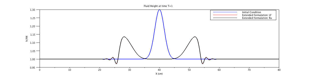
Fig. 1: Profile of the surface of the fluid at time $T=1$

In figure 2, we have drawn the relative entropy $\frac{U}{U|_{t=0}}$ as a function of time: the picture clearly indicates that the difference approximation of the extended formulation have better entropy stability properties than difference approximation of (38).

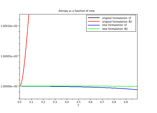
Fig. 2: Entropy as a function of time: Comparison of the various discretizations of (38).

A natural question arises about the new formulation: indeed one may ask whether the relation $hw=\frac{2}{3}\sqrt{\kappa}\partial_{x}(h^{3/2})$ is satisfied for all time. If not, it does not make sense to compare the performance with respect to entropy stability since it would represent two distinct quantities. In figure 3, we draw the relative error at time $T=1$ and defined as

$${\displaystyle err_{j}=\frac{|(hw)_{j}-\sqrt{\kappa}\frac{h_{j+1}^{3/2}-h_{j-1}^{3/2}}{3\delta x}|}{\|hw\|},\quad j=1,\dots,N.}$$

The numerical simulations show very good agreement, especially for the less dissipative scheme, Rusanov, than for Lax Friedrichs scheme. We have also implemented an alternative scheme where the relation $hw=\frac{2}{3}\sqrt{\kappa}\partial_{x}(h^{3/2})$ is enforced at each time step: we have not noticed any change in the numerical solution.

The CFL condition found for Rusanov scheme is of the form $\delta t=O(\delta x^{7/3})$ that is rather close to the “optimal” heuristic CFL condition $\delta t=O(\delta x^{2})$. Therefore, we can conclude that a difference approximation of the extended formulation of (38) with a Rusanov flux and second order accurate both in time and space is a natural candidate to perform numerical simulations of falling films experiments by Liu and Gollub [LG].

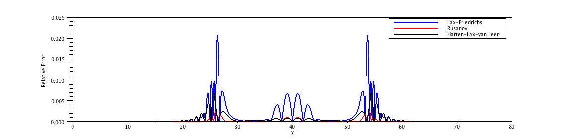
Fig. 3: Consistency of the new formulation: relative error between the new variable $hw$ and $\frac{2}{3}\sqrt{\kappa}\partial_{x}(h^{3/2})$. The Rusanov scheme and the Harten Lax Van Leer scheme have comparable consistency properties. In regards, the Lax Friedrichs scheme is less efficient to preserve consistency

4.2 Hamiltonian discretization and dispersive shock waves

In what follows, we have tested the difference hamiltonian approximation of (38). The initial conditions are the same than in the previous section. In order to be entropy stable it is necessary to employ an implicit method: we have used here an implicit backward Euler time discretization. Due to the nonlinearity of the problem, the Crank Nicolson, second order accurate, time discretization does not guarantee entropy stability. Therefore, we did not try to compare with other schemes tested in the previous section. An important remark is that now there is no numerical viscosity: a drawback is that the dynamical behavior is completely changed as shown in figure 4 in comparison to what is found in the presence of numerical viscosity (figure 1).

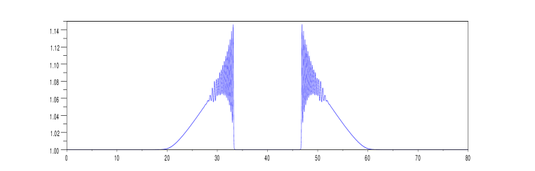
Fig. 4: Fluid height profile at time T=0.66: the oscillatory zone is increasing with time, characteristic of a dispersive shock wave

In order to see whether it is a numerical artifact, we checked the entropy stability of the difference hamiltonian approximation: the entropy remains clearly bounded with time. Indeed, these oscillations are not a numerical artifact and can be explained (formally) by the theory of dispersive shock waves. Here, the classical hyperbolic shocks are smoothed by disperses effects: the oscillatory zone grows up in time and the oscillations are described by the Whitham modulations equations. This picture is not valid anymore in the presence of a slight amount of viscosity: there are still some oscillations but the width of the oscillatory zone stops growing after some time: see [J] and [EGK] for a detailed analysis respectively in the case of the Korteweg de Vries/Burgers equation and in the case of the Kaup system perturbed by a viscous term. Here the physical viscosity is replaced by numerical viscosity.

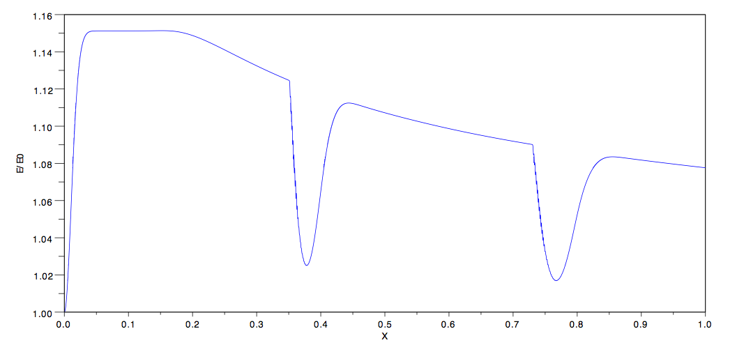
Fig. 5: Entropy as a function of time. The behavior is rather similar to difference approximations in original variables: the entropy first increases then decreases with time: the “holes” in the decreasing part of the curve correspond to times when the bumps interact

4.3 Simulation of a Liu-Gollub experiment

In this section, we show a numerical simulation for a shallow water model derived for thin film flows down an inclined plane. The model is written as (see [BN] for more details)

$$\begin{array}[]{ll}\displaystyle\partial_{t}h+\partial_{x}(hu)=0,\\ \displaystyle\partial_{t}(hu)+\partial_{x}\left(hu^{2}+P(h)\right)=\frac{2}{9\varepsilon Re}(h-\frac{u}{h})+\frac{\varepsilon}{We}h\partial_{xxx}h+\frac{6\varepsilon}{Re}\partial_{xx}(hu),\end{array}$$ (39)

with $P(h)$ is a pressure term given by $\displaystyle P(h)=\frac{h^{2}}{2F^{2}}+\frac{2h^{5}}{25}.$ The non dimensional $Re$, $F^{2}$, $We$ and $\varepsilon$ are, respectively the Reynolds, Froude and Weber numbers and the aspect ratio. Once $Re$ is fixed, we define $h_{N},u_{N},F^{2}$ and $We$ as

$$h_{N}=\left(\frac{2Re\nu^{2}}{g\sin\theta}\right)^{\displaystyle\frac{1}{3}},u_{N}=\nu\frac{Re}{h_{N}},\quad F^{2}=\frac{2}{9}Re\tan(\theta),\quad We=\frac{\rho\lambda u_{N}^{2}}{\sigma}$$

with $\lambda$ a characteristic wavelength of the flow, $\sigma$ represents the surface tension of the fluid, $\nu$ its viscosity and $\rho$ its density. Since the capillary ripples found in [LG] are of order $1cm$, we choose $\lambda=0.01$. The characteristic time scale is $T_{N}=\lambda/u_{N}$. In [LG], the Reynolds number in the experiment is $Re=29$ whereas $g=9.8$, $\rho=1134$, $\theta=6.4^{o}$, $\sigma=6.7\times 10^{-2}$ and $\nu=6.28\times 10^{-6}$. Then, one finds

$$h_{N}\approx 1.28\times 10^{-3},\>\>u_{N}\approx 9.49\times 10^{-2},\>\>T_{N}\approx 0.105,\>\>F^{2}\approx 0.723,\>\>We\approx 1.52.$$

Note that the viscous term $(6\varepsilon/Re)\partial_{xx}(hu)$ is only heuristic so that the model is not a second order accurate model (with respect to the aspect ratio $\varepsilon=h_{N}/\lambda$).The frequency of the perturbation at the inlet is $f=1.5Hz$. At time $t=0$, the fluid height and velocity are constant $h=1$ and $u=1$. Following the conclusions of our study, we have chosen to carry out numerical simulations with a fully second order accurate scheme of the extended formulation of (39) and used a Rusanov flux for the first order part. Our numerical results show a good agreement with the experiment by Liu and Gollub [LG].

Up to now, the choice of boundary conditions for the Euler Korteweg equations on a finite interval is an open problem so that we have chosen rather arbitrary boundary conditions. Furthermore, since the difference scheme contains numerical/physical viscosity, we have considered a set of $5$ boundary conditions. First, at the inlet, we chose: ${\displaystyle h|_{x=0}=1+0.03\sin(2\pi\,f\,T_{N}t),\quad hu|_{x=0}=1,\quad\partial_{x}h|_{x=0}=0.}$ In contrast to [KRSV], we have chosen free boundary conditions at the outlet:

$${\displaystyle\partial_{x}h|_{x=L}=\partial_{x}(hu)|_{x=L}=0}$$

instead of “hyperbolic type” boundary conditions where $h$ and $hu$ are convected with an artificial velocity $V_{out}>0$. As pointed out in [KRSV] the choice of the boundary conditions at the outlet does not seem to influence the dynamic within the channel (no reflection waves).

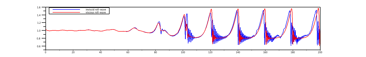
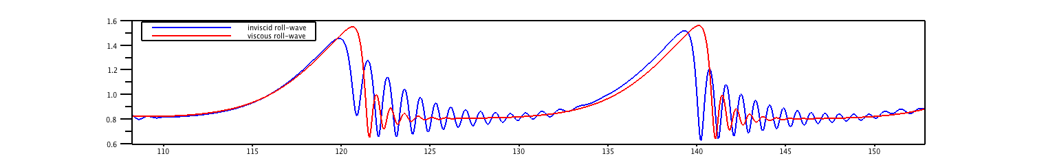
Fig. 6: Simulation of Liu Gollub experiment [LG]: the Reynolds number is $Re=29$ and the inclination is $\theta=6.4^{o}$. The frequency at the inlet if $f=1.5Hz$. On top: a picture of the complete experiment, from the inlet to the outlet (2m). On below: a zoom over one spatial period when roll-wave profiles are stabilized

5 Concluding remarks

In this paper, we considered the stability of various difference approximations of the Euler Korteweg equations with applications to shallow water equations with surface tension. A first class of difference approximations is built by considering the Euler Korteweg system as the classic isentropic compressible Euler equations perturbed by a disperse term. This latter term is discretized with centered finite differences and various classical scheme for the convection part are considered. It is proved that a certain amount of numerical viscosity is needed to obtain difference schemes that are stable in the von Neumann sense (under suitable CFL conditions).

In order to get entropy stability, we considered an extended formulation of the Euler Korteweg equations and proved entropy stability of Lax Friedrichs type schemes whereas Roe/Godunov schemes are always unstable with forward Euler explicit discretization. We have shown numerically that the extended formulation of the Euler Korteweg system has better stability properties than the original one. We also carry out a numerical simulation of a shallow water system which models an experiment by Liu and Gollub to observe roll-waves [LG].

By considering the Euler Korteweg system as a Hamiltonian system of evolution PDEs, we introduced a semi-discretized difference approximations which preserves the Hamiltonian structure. This scheme has no numerical viscosity so that it is particularly useful to study purely dispersive Euler Korteweg system: in particular, one can find numerically the dispersive shock waves [E] of the Euler Korteweg system.

Several questions remain open. First, we carried out a numerical simulation of an experiment of Liu and Gollub [LG] by choosing arbitrary boundary conditions. In fact, the choice of suitable boundary conditions for the Euler Korteweg system on a finite interval in order to prove well posedness is still an open problem. A first attempt in this direction is found in [A] where the well posedness of the linearized Euler Korteweg equations is proved on a half space under a generalized Lopatinskii condition.

Furthermore, we restricted our attention to one dimensional problem. For thin film flows, this restricts the study to primary instabilities: in order to analyze secondary instabilities found, one has consider $2d$ problems. In that setting, an extended formulation is still available [BDDd] so that we expect our analysis extends easily, at least to cartesian meshes. An other interesting question is the extension of this analysis to other mixed hyperbolic/dispersive equations like the Boussinesq equations or the Serre/Green-Naghdi equations. Up to now, the strategy adopted to deal with these system is time splitting without proof of stability (though numerical results are rather satisfying).

Finally an other open interesting question concerns the time integration of the hamiltonian semi-discrete approximation: here, we have used a backward Euler time integration so as to be entropy stable but it does not preserve the hamiltonian (nor a perturbation of it). Instead, one should consider symplectic time integration scheme, in particular but using various splitting. This kind of method are particularly of interest in order to study the nonlinear stability of various traveling waves solutions of the purely dispersive equations.

References

- [A] C. Audiard Non homogeneous boundary value problems for linear dispersive equations, Comm. Parti. Diff. Eqs 37 (2012) no 1, p. 1-37
- [BDD] S. Benzoni-Gavage, R. Danchin, S. Descombes Well-posedness of one-dimensional Korteweg models, Electronic J. Diff. Equations 59 (2006), pp. 1-35.
- [BDDd] S. Benzoni-Gavage, R. Danchin, S. Descombes On the well-posedness for the Euler-Korteweg model in several space dimensions, Indiana Univ Math Journal 56 (2007), no 4, pp. 1499-1579.
- [BDK] D. Bresch, B. Desjardins, C.K. Lin On some compressible fluid models: Korteweg, Lubrication and Shallow Water systems Comm. Part. Diff Eqs 28 (2003) no. 3-4, p. 843-868.
- [BN] D. Bresch, P. Noble Mathematical Justification of a shallow water model, Methods and Applications of Analysis 14 (2007) no. 2, p. 87-117.
- [CDS] R. Carles, R. Danchin, J.-C. Saut Madelung, Gross-Pitaevskii and Korteweg (2011) arXiv:1111.4670.
- [CL] C. Chalons, P.G. LeFloch High-Order Entropy-Conservative Scheme and Kinetic Relations for Van der Waals Fluids, Journal of Computational Physics 168 (2001) 184-206.
- [Col] F. Coquel, P.G. LeFloch An entropy satisfying MUSCL scheme for systems of conservation laws Numer. Math. 74 (1996) 1-33.
- [E] G. A. El, Resolution of a shock in hyperbolic systems modified by weak dispersion Chaos, 15 (3): 037103, 21, 2005.
- [EGK] G. A. El, R. H. J. Grimshaw, and A.M. Kamchatnov, Analytic model for a weakly dissipative shallow water undular bore Chaos, 15 (3): 037102, 2005.
- [EGS] G. A. El, R. H. J. Grimshaw, and N. F. Smyth. Unsteady undular bores in fully nonlinear shallow-water theory. Physics of Fluids, 18(2):027104, February 2006.
- [HR] J. Haink, C. Rohde Local Discontinuous-Galerkin Schemes for Model Problems in Phase Transition Theory Commun. Comput. Phys, 4 (2008) no 4, p. 860-893.
- [HAC] M.A. Hoefer, M.J. Ablowitz, I. Coddington, E.A. Cornell, P. Engels, V. Schweikhard Dispersive and classical shock waves in Bose-Einstein condensates and gas dynamics Physical Review A 74 (2006) no 2, 023623.
- [JTB] D. Jamet, D. Torres and J.U. Brackbill On the theory and Computation of Surface Tension: The elimination of Parasitic Currents through Energy Conservation in the Second-Gradient Method Journal of Computational Physics 182 (2002) 262-276.
- [J] S. Johnson A non-linear equation incorporating damping and dispersion J. Fluid. Mech. 42 (1970) p. 49-60.
- [KRSV] S. Kalliadasis, C. Ruyer-Quil, B. Scheid, M.G. Velarde Falling Liquid Films, Applied Mathematical Sciences 176 (2012)
- [LMR] P.G. LeFloch, J.M. Mercier, C. Rohde Fully discrete, entropy conservative schemes of arbitrary order, SIAM J. Numer. Anal. 40 (2002) No 5, pp 1968-1992.
- [LG] J. Liu, J.P. Gollub Solitary wave dynamics of film flows, Phys. Fluids 6, 1702 (1994).
- [NV] P. Noble, J.-P. Vila Consistency, Stability, Gallilean indifference criteria for design of Two moments closure equations of Shallow water type for Thin Film laminar flow gravity driven. in preparation.
- [VL] B. Van Leer Towards the ultimate conservative difference schemes: a second order sequel to Godunov’s method J. Comp. Phys 43 (1981) 357-372.
- [T] E. Tadmor Entropy stability theory for difference approximations of nonlinear conservation laws and related time-dependent problems Acta Numerica (2003) pp. 451-512.
- [YS] J. Yan, C.-W. Shu A local discontinuous galerkin method for KdV type equations SIAM J. Numer Anal 40 (2002) no. 2, p. 769-791.