Extremely efficient generation of Gamma random variables for $\alpha\geq 1$

Abstract

The Gamma distribution is well-known and widely used in many signal processing and communications applications. In this letter, a simple and extremely efficient accept/reject algorithm is introduced for the generation of independent random variables from a Gamma distribution with any shape parameter $\alpha\geq 1$. The proposed method uses another Gamma distribution with integer $\alpha_{p}\leq\alpha$, from which samples can be easily drawn, as proposal function. For this reason, the new technique attains a higher acceptance rate (AR) for $\alpha\geq 3$ than all the methods currently available in the literature, with $\textrm{AR}\to 1$ as $\alpha\to\infty$.

I Introduction

The Gamma probability density function (PDF) is given by $p_{o}(x)=C_{1}p(x)$, with $C_{1}=\frac{\beta^{\alpha}}{\Gamma(\alpha)}$, and

$$p(x)=x^{\alpha-1}\exp\left(-\beta x\right),\qquad x\geq 0,$$ (1)

where $\alpha>0$ is the shape parameter, $\beta>0$ is the rate parameter and $\Gamma(\alpha)$ is the Gamma function [6, Chapter 4]. The Gamma distribution is well-known and widely used in different fields, such as Bayesian inference [10], signal processing [11] and digital communications [14]. In particular, in communications it has been recently applied in the simulation of fading/shadowing channels using the Weibull-Gamma model [4, 2] or the effects of the turbulent atmosphere in free-space optical links with the Gamma-Gamma approach, which requires two independent Gamma random variables [9, 13].

All of the aforementioned applications need the generation of independent Gamma random variables (RVs), $X$, with arbitrary values of $\alpha$ and $\beta$, i.e., $X\sim G(\alpha,\beta)$. When $\alpha$ is an integer, an exact sampler is available. Indeed, if $\alpha=n\in\mathbb{N}^{+}$ the Gamma PDF becomes an Erlang PDF [6], and $X$ can be generated as the sum of $n=\alpha$ independent exponential RVs, i.e., $X=\sum_{i=1}^{n}E_{i}$, where each $E_{i}$ follows an exponential PDF with parameter $\beta$. These exponentials can be easily obtained through the inversion method [6, Chapter 3], allowing us to express $X$ as

$$X=-\frac{1}{\beta}\sum_{i=1}^{\alpha}{\ln\left(U_{i}\right)}=-\frac{1}{\beta}\ln\left(\prod_{i=1}^{\alpha}U_{i}\right),$$ (2)

where the $U_{i}$ are uniform RVs, i.e., $U_{i}\sim\mathcal{U}([0,1])$. For $\alpha\notin\mathbb{N}^{+}$, the problem of generating a Gamma RV $X$ is usually divided in two subcases: $\alpha<1$ and $\alpha\geq 1$. Focusing on the second case, which is the one addressed in this paper, we note that an exact sampler does not exist, but several accept/reject methods have been introduced (see [6, 8, 7] for a review of the approaches proposed). Most of these methods consider only $\beta=1$, since, given $\widetilde{X}\sim G(\alpha,1)$, it can be easily shown that $X=\frac{1}{\beta}\widetilde{X}\sim G(\alpha,\beta)$.

In this letter, we develop an extremely efficient rejection sampler to draw independent samples from a Gamma PDF with $\alpha\geq 1$ and any value of $\beta$. The proposed method outperforms all the alternative techniques reported in the literature in terms of acceptance rate (i.e., the key performance measure of a accept/reject methods) for $\alpha\geq 3$. The main idea is using a suitable Gamma PDF with an integer $\alpha_{p}\leq\alpha$ as a proposal density, from which samples can be easily drawn using Eq. (2). Since the proposal is itself another Gamma PDF, it provides a very good fit of the target, thus attaining very high acceptance rates that tend to $100\%$ for $\alpha\rightarrow+\infty$, i.e., virtually providing exact sampling.

II Background: accept/reject algorithm

Rejection sampling (RS) is a classical technique for generating independent samples from an arbitrary target PDF, $p_{o}(x)=C_{1}p(x)$ with $x\in\mathcal{D}$ and $C_{1}=[\int_{\mathcal{D}}p(x)dx]^{-1}$, using an alternative simpler proposal PDF, $\pi_{o}(x)=C_{2}\pi(x)$ with $x\in\mathcal{D}$ and $C_{2}=[\int_{\mathcal{D}}\pi(x)dx]^{-1}$, such that $\pi(x)\geq p(x)$, i.e., $\pi(x)$ is a hat function w.r.t. $p(x)$. RS works by generating samples from the proposal density, $x^{\prime}\sim\pi_{o}(x)$, accepting them when $u^{\prime}\leq p(x^{\prime})/\pi(x^{\prime})$, with $u^{\prime}\sim\mathcal{U}([0,1])$, and rejecting them otherwise. The key performance measure for RS is the average acceptance rate (AR), $a_{R}=\int_{\mathcal{D}}\frac{p(x)}{\pi(x)}\pi_{o}(x)dx=\frac{C_{2}}{C_{1}}\leq 1$. The value of $a_{R}$ depends on how close the proposal is to the target, and determines the efficiency of the approach. Hence, the main difficulty when designing an RS algorithm is finding a good hat function, $\pi(x)\geq p(x)$, such that $\pi(x)$ and $p(x)$ are as close as possible and drawing samples from $\pi_{o}(x)=C_{2}\pi(x)$ can be done easily and efficiently.

III Novel technique

In this letter, we consider as target density the PDF given in Eq. (1) with $\alpha\geq 1$ and any $\beta>0$. As proposal PDF, we suggest using another Gamma density with different parameters, namely,

$$\pi_{o}(x)\propto\pi(x)=K_{p}\mbox{ }x^{\alpha_{p}-1}\exp\left(-\beta_{p}x\right),\qquad x\geq 0,$$ (3)

where $\alpha_{p}=\lfloor\alpha\rfloor\leq\alpha$, with $\lfloor\alpha\rfloor$ denoting the integer part of $\alpha\in[1,+\infty)$, and the remaining parameters ($\beta_{p}$ and $K_{p}$) adjusted to obtain the same location and value of the maximum for the proposal and the target. On the one hand, for $\alpha\geq 2$,

$$\beta_{p} =\frac{\alpha_{p}-1}{x_{\max}}=\beta\frac{\alpha_{p}-1}{\alpha-1},$$ (4)

$$K_{p} =\frac{p(x_{\max})}{x^{\alpha_{p}-1}\exp\left(-\beta_{p}x\right)}$$

$$=\exp\left(\alpha_{p}-\alpha\right)\left(\frac{\alpha-1}{\beta}\right)^{(\alpha-\alpha_{p})},$$ (5)

where $x_{\max}=\frac{\alpha-1}{\beta}$ is the location of the single maximum of the Gamma PDF, obtained solving $\frac{dp(x)}{dx}=0$. For $1\leq\alpha<2$, $\alpha_{p}=1$, we set

$$\beta_{p} =\frac{\beta}{\alpha},$$ (6)

$$K_{p} =\exp(1-\alpha)\left(\frac{\alpha}{\beta}\right)^{\alpha-1}.$$ (7)

In this case, they are obtained finding the exponential function tangent to $p(x)$ at the optimal point

$$x^{*}=\frac{\alpha}{\beta}.$$

This is an optimal value since it maximizes the acceptance rate, as shown in the Appendix -A. When $\alpha=1$, the parameters are $\alpha_{p}=\alpha$, $\beta_{p}=\beta$ and $K_{p}=1$. In this case the unique intersection point between $\pi(x)$ and $p(x)$ is $x^{*}$. The values in Eqs. (6)-(7) can be easily obtained analytically computing the tangent straight line to the function $\log[p(x)]$ at $x^{*}$ (note that the Gamma pdf is a log-concave density).

Thanks to this choice of $\alpha_{p}$ and the parameters derived in Eqs. (4)-(5)-(6) and (7), we can ensure that: (a) we can draw samples exactly from $\pi_{o}(x)\propto\pi(x)$ [6]; (b) $\pi(x)\geq p(x)$ for all $x\geq 0$, as proved in the following section. Figure 1 depicts some examples of envelope and target functions with different values of the parameters.

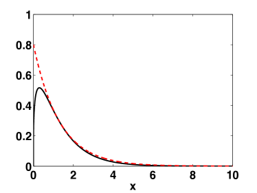
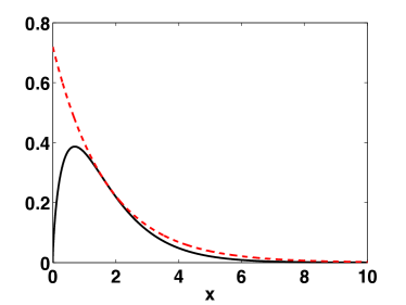
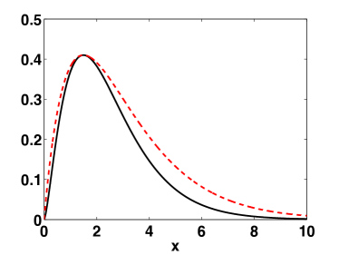
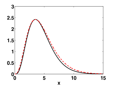
Figure 1: The target function $p(x)$ (solid line) and the proposed envelope function $\pi(x)$ (dashed line) with different values of the parameters: (a) $\alpha=1.3$, $\beta=1$, (b) $\alpha=1.7$, $\beta=1$, (c) $\alpha=2.5$, $\beta=1$ and (d) $\alpha=4.5$, $\beta=1$.

Our algorithm can be summarized in the following three steps: (1) calculate the parameters of the proposal PDF, $\pi_{o}(x)\propto\pi(x)$; (2) draw a sample $x^{\prime}$ from $\pi_{o}(x)$ using the direct approach described in Eq. (2), i.e., generate $\alpha_{p}$ independent uniform RVs, $u_{i}\sim\mathcal{U}([0,1])$ with $i=1,...,\alpha_{p}$, and set

$$x^{\prime}=-\frac{1}{\beta_{p}}\ln\left(\prod_{i=1}^{\alpha_{p}}u_{i}\right);$$ (8)

(3) accept $x^{\prime}$ with probability $p(x^{\prime})/\pi(x^{\prime})$, discarding it otherwise. Repeat steps (2) and (3) until the desired number of samples have been obtained.

IV Proof of the RS inequality

IV-A Case $\alpha\geq 2$

Consider first the proposal pdf for $\alpha\geq 2$.In order to apply the RS technique, we need to ensure that $\pi(x)\geq p(x)$, i.e.,

$$K_{p}x^{\alpha_{p}-1}\exp\left(-\beta_{p}x\right)\geq x^{\alpha-1}\exp\left(-\beta x\right),\qquad\forall x\geq 0.$$ (9)

For $x>0$, Eq. (9) can be rewritten alternatively as

$$K_{p}\exp\left(\Omega x\right)\geq x^{\alpha-\alpha_{p}},$$ (10)

where $\Omega\triangleq\beta-\beta_{p}$ and $x^{\alpha-\alpha_{p}}$ presents a sub-linear growth, since $0\leq\alpha-\alpha_{p}<1$. Finally, taking the logarithm on both sides of (10),

$$\ln(K_{p})+\Omega x\geq(\alpha-\alpha_{p})\ln(x).$$ (11)

Now, since $\alpha\geq\alpha_{p}$ and $\beta_{p}$ is given by (4), we note that

$$\Omega=\beta-\beta_{p}=\beta\left(1-\frac{\alpha_{p}-1}{\alpha-1}\right)\geq 0.$$ (12)

Hence, the linear function on the left hand side of (11) is increasing. Moreover, since $\alpha\geq\alpha_{p}$, the logarithmic function on the right hand side of (11) is increasing and . Consequently, since both functions are increasing and concave for $x>0$ (i.e., their second derivatives are lower or equal than zero), they can have at most two intersection points. Indeed, in the sequel we show that they are tangent at $x=x_{\max}$, which is the only contact point between both curves for $x>0$. In order to prove this, we need to show: (1) that both functions are equal at $x=x_{\max}$, i.e.,

$$\ln(K_{p})+\Omega x_{\max}=(\alpha-\alpha_{p})\ln(x_{\max})=(\alpha-\alpha_{p})\ln\left(\frac{\alpha-1}{\beta}\right),$$ (13)

which is fulfilled by construction of the proposal, as $K_{p}$ and $\beta_{p}$ are set to achieve $\pi(x_{\max})=p(x_{\max})$; (2) that their first derivatives are equal, i.e.,

$$\frac{d(\ln(K_{p})+\Omega x)}{dx}\Bigg{|}_{x=x_{\max}}=\frac{d((\alpha-\alpha_{p})\ln x)}{dx}\Bigg{|}_{x=x_{\max}},$$ (14)

and taking the derivatives we obtain

$$\Omega=\frac{\alpha-\alpha_{p}}{x_{\max}}=\frac{\beta(\alpha-\alpha_{p})}{\alpha-1}=\beta\left(1-\frac{\alpha_{p}-1}{\alpha-1}\right),$$ (15)

which is the result given by Eq. (12).

Consequently, since $x$ grows faster than $\ln(x)$, we can guarantee that $\ln(K_{p})+\Omega x\geq(\alpha-\alpha_{p})\ln(x)$ for $x>0$, with equality only at $x=x_{\max}$. Hence, the RS inequality in (9) is satisfied and the proposal is indeed a hat function for $p(x)$, i.e., $\pi(x)\geq p(x)$, with equality only at $x=0$, $x=x_{\max}$ and $x\to+\infty$.

IV-B Case $1\leq\alpha<2$

For, $1\leq\alpha<2$, we have $\alpha_{p}=1$ and the proposal pdf is built computing the tangent straight line $r(x)=-\beta_{p}x+\log[K_{p}]$ tangent to $\log[p(x)]$ at a generic point $x^{*}$ (for the optimal choice of this point, see the Appendix -A). Then, the envelope function is

$$\pi(x)=\exp(r(x))=K_{p}\exp(-\beta_{p}x).$$

For the log-concavity of $p(x)$, i.e.,

$$\frac{d^{2}\log[p(x)]}{dx^{2}}\geq 0,$$

we have

$$r(x)\geq\log[p(x)],$$

and since the exponential function is a monotonically increasing transformation, we have $\pi(x)\geq p(x)$, that is the needed condition to apply the RS technique.

V Acceptance rate of the novel RS scheme

The acceptance rate of the novel scheme can be calculated analytically. Indeed, in general, we have

$$a_{R}=\frac{\int_{0}^{+\infty}p(x)dx}{\int_{0}^{+\infty}\pi(x)dx},$$

so that

$$a_{R}=\left\{\begin{split}\frac{\Gamma(\alpha)}{\alpha^{\alpha}e^{1-\alpha}},\quad\quad\quad\quad\quad&\mbox{ for }1\leq\alpha<2,\\ \left(\frac{e}{\alpha-1}\right)^{(\alpha-\alpha_{p})}\frac{\Gamma(\alpha)}{\Gamma(\alpha_{p})},\quad&\mbox{ for }\alpha\geq 2,\end{split}\right.$$ (16)

that is independent from the parameter $\beta$.

VI Results

Gamma generators in the literature are usually designed and compared for $\beta=1$, without loss of generality. Hence, in order to obtain a fair comparison we only consider $\beta=1$, although our approach is valid for any value of $\beta$. We have compared the acceptance rate (AR), $a_{R}$, of the different algorithms described below [6, 8, 7]:

• Our method (M1): For $1\leq\alpha<2$, the AR is indicated as $a_{R1}$ and is given in Eq. (16). Note that, for $\alpha\rightarrow+\infty$, we obtain $a_{R1}\rightarrow 1$, i.e., our approach provides exact sampling asymptotically.

• Log-logistic method  (M2) [5]: The proposal PDF is $\pi(x)=K_{1}\frac{x^{\lambda-1}}{(\mu+x^{\lambda})}$, with $\lambda=\sqrt{2\alpha-1}$, $\mu=\alpha^{\lambda}$ and $K_{1}=4\alpha^{(\alpha+\lambda)}e^{-\alpha}$. The theoretical AR is $a_{R2}=\frac{\Gamma(\alpha)\mu\lambda}{K_{1}}$. For $\alpha\rightarrow+\infty$, $a_{R2}\rightarrow\frac{\sqrt{\pi}}{2}\approx 0.88$.

• Cauchy method (M3) [1]: The proposal is $\pi(x)=K_{2}\frac{\lambda}{\lambda^{2}+(x-a)^{2}}$, with $\lambda=\sqrt{2\alpha-1}$, $a=\alpha-1$ and $K_{2}=\frac{c}{2\pi}\lambda(a-1)^{(a-1)}e^{1-a}$, where $c=\pi+2\arctan(a/\lambda)$. The AR is $a_{R3}=\frac{\Gamma(\alpha)}{\pi K_{2}}$ and we have $a_{R3}\rightarrow\frac{1}{\sqrt{\pi}}\approx 0.56$, for $\alpha\rightarrow+\infty$.

• T-student method (M4) [3]: The proposal is $\pi(x)=K_{3}(1+0.5(\frac{x-\alpha+1}{\eta})^{2})^{-3/2}$ with $\eta=\sqrt{\frac{3\alpha-0.75}{2}}$ and $K_{3}=(\alpha-1)^{\alpha-1}e^{1-\alpha}$. It can be shown that $a_{R4}\rightarrow\sqrt{\frac{\pi}{6}}\approx 0.72$ for $\alpha\rightarrow+\infty$.

• Modified Ratio-of-Uniforms (RoU) (M5) [12]: It is a variant of the RoU scheme [6, 8], relocating the mode of $p(x)$ at $x=0$. The asymptotic AR is $a_{R4}\rightarrow\frac{\sqrt{e\pi}}{4}\approx 0.73$, for $\alpha\rightarrow+\infty$. The AR, $a_{R4}$, is almost constant for all values of $\alpha>1$, as shown in Figure 2.

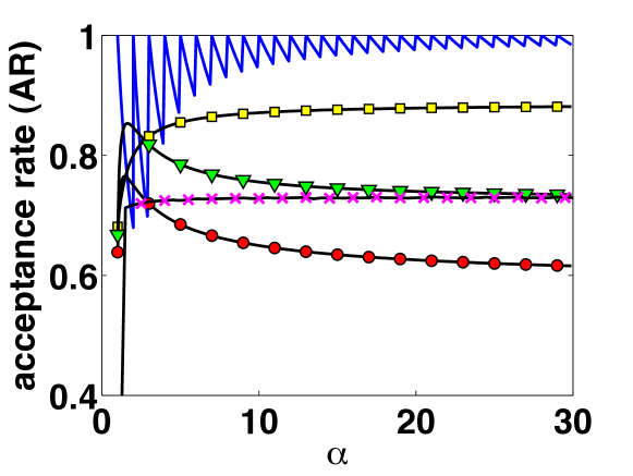
Figure 2: Acceptance rate (AR) using our method M1 (continuous line), M2 (squares), M3 (circles), M4 (triangles) and M5 (x-marks), for $1\leq\alpha\leq 30$ and $\beta=1$.

Figure 2 shows the ARs of all the techniques described above, obtained empirically after drawing $N=6\cdot 10^{5}$ independent samples, for different values of $\alpha$. For $1\leq\alpha\leq 1.35$ our the technique M1 provide the best results whereas for $1.35\leq\alpha\leq 2$ the best technique is M4. For $2\leq\alpha\leq 2.37$ the newly proposed approach (M1) provides the highest AR while for $2.37<\alpha<3$, the best method is M2 or M4 depending of the value of $\alpha$. For $\alpha\geq 3$, our technique (M1) is extremely efficient, outperforming (expect for $3.87\leq\alpha<4$ where M2 is slightly better) the rest of the methods and providing the best results ever reported in the literature. The minimum AR obtained with M1 is $\approx 0.68$ for $\alpha\approx 1.99$. Furthermore, our technique provides exact sampling (i.e., $a_{R1}\to 1$) asymptotically as $\alpha\rightarrow+\infty$.

VII Conclusions

We have developed a rejection sampling (RS) scheme for generating Gamma random variables, with arbitrary values of $\alpha\geq 1$ and $\beta$, where the proposal PDF is itself another Gamma density. The proposed algorithm is simple and extremely efficient, providing the best acceptance rates ever reported in the literature for $\alpha\geq 3$.

VIII Acknowledgement

This work has been partly financed by the Spanish government, through the CONSOLIDER-INGENIO 2010 program (CSD2008-00010), as well as projects COMPREHENSION (TEC2012-38883-C02-01) and DISSECT (TEC2012-38058-C03-01).

-A Optimal choice of the tangent point for $1\leq\alpha<2$

First, we recall the notation $p_{o}(x)=C_{1}p(x)$ with

$$C_{1}=\left[\int_{\mathcal{D}}p(x)dx\right]^{-1},$$

and $\pi_{o}(x)=C_{2}\pi(x)$ with

$$C_{2}=\frac{1}{I_{\pi}}=\left[\int_{\mathcal{D}}\pi(x)dx\right]^{-1}.$$

The acceptance rate (AR) is

$$\begin{split}a_{R}&=\int_{\mathcal{D}}\frac{p(x)}{\pi(x)}\pi_{o}(x)dx\\ &=\frac{\int_{\mathcal{D}}p(x)dx}{\int_{\mathcal{D}}\pi(x)dx}=\frac{C_{2}}{C_{1}}=\frac{1}{C_{1}I_{\pi}}\leq 1.\end{split}$$ (17)

Since the are below the target $p(x)$ is given (then fixed), the only way to increase the AR is diminishing the area $I_{\pi}$ below the envelope function, i.e., we desire to build a function $\pi(x)$ such that satisfies jointly both conditions

$$\left\{\begin{split}&I_{\pi}^{*}=\min_{\pi(x)}\int_{\mathcal{D}}\pi(x)dx,\\ &\pi(x)\geq p(x).\end{split}\right.$$ (18)

For $1\leq\alpha<2$, the novel technique uses as proposal function of the form in Eq. (3) with $\alpha_{p}=1$, and the other parameters, as function of a generic tangent point $\theta$, are

$$\beta_{p}(\theta)=-\frac{\alpha-1}{\theta}+\beta,\quad\quad\theta\neq 0$$

$$K_{p}(\theta)=\theta^{\alpha-1}e^{1-\alpha}.$$

Therefore, our proposal for $1\leq\alpha<2$ has the following form

$$\pi(x)=K_{p}(\theta)\exp\left(-\beta_{p}(\theta)x\right),\quad x\in\mathcal{D}=\mathbb{R}^{+},\quad\theta\in\mathbb{R}^{+}\setminus\{0\},$$

then

$$\begin{split}I_{\pi}(\theta)&=\int_{0}^{+\infty}K_{p}(\theta)\exp\left(-\beta_{p}(\theta)x\right)dx=\frac{K_{p}(\theta)}{\beta_{p}(\theta)}\\ &=\frac{\theta^{\alpha-1}e^{1-\alpha}}{-\frac{\alpha-1}{\theta}+\beta},\quad\theta\neq 0.\end{split}$$ (19)

The value of $\theta$ that minimizes $I_{\pi}(\theta)$ is a solution of the equation

$$\begin{split}&\frac{dI_{\pi}(\theta)}{d\theta}=0,\\ &\frac{\theta^{\alpha-1}(\alpha-\beta\theta)(1-\alpha)e^{1-\alpha}}{(\beta\theta-\alpha+1)^{2}}=0.\end{split}$$ (20)

The solution are $\theta^{*}=0$ (that is not admissible) and

$$x^{*}=\theta^{*}=\frac{\alpha}{\beta}.$$

Choosing this value $x^{*}$ as tangent point to construct the envelope function,

$$\pi(x)=\left(\frac{\alpha}{\beta}\right)^{\alpha-1}e^{1-\alpha}\exp\left(-\frac{\beta}{\alpha}x\right),$$

we maxime the AR of the RS scheme. Since $C_{1}=\frac{\beta^{\alpha}}{\Gamma(\alpha)}$, the AR in this case is

$$\begin{split}a_{R}&=\frac{\Gamma(\alpha)\beta_{p}(x^{*})}{\beta^{\alpha}K_{p}(x^{*})}\\ &=\frac{\Gamma(\alpha)\frac{\beta}{\alpha}}{\beta^{\alpha}\left(\frac{\alpha}{\beta}\right)^{\alpha-1}e^{1-\alpha}}=\frac{\Gamma(\alpha)}{\beta^{\alpha}\left(\frac{\alpha}{\beta}\right)^{\alpha}e^{1-\alpha}}\\ &=\frac{\Gamma(\alpha)}{\alpha^{\alpha}e^{1-\alpha}},\end{split}$$ (21)

independent from the parameter $\beta$.

References

• [1] J.ย H. Ahrens and U.ย Dieter. Computer methods for sampling from gamma, beta, poisson and binomial distributions. Computing, 12:223โ€“246, 1974.
• [2] J.ย A. Anastasov, G.ย T. Djordjevic, and M.ย C. Stefanovic. Outage probability of interference-limited system over Weibull-gamma fading channel. Electronics Letters, 48(7):408โ€“410, March 2012.
• [3] D.ย J. Best. Letter to the editors. Appl. Stat., 29:181โ€“182, 1978.
• [4] P.ย S. Bithas. Weibull-gamma composite distribution: alternative multipath/shadowing fading model. Electronics Letters, 45(14):749โ€“751, July 2009.
• [5] R.ย C.ย H. Cheng. The generation of gamma variables with non-integral shape parameter. Appl. Stat., 26:71โ€“75, 1977.
• [6] J.ย Dagpunar. Principles of random variate generation. Clarendon Press (Oxford and New York), New York, 1988.
• [7] J.ย Dagpunar. Simulation and Monte Carlo: With applications in finance and MCMC. John Wiley and Sons, Ltd, England, 2007.
• [8] L.ย Devroye. Non-Uniform Random Variate Generation. Springer, 1986.
• [9] W.ย Gappmair and S.ย S. Muhamad. Error performance of PPM/Poisson channels in turbulent atmosphere with gamma-gamma distribution. Electronics Letters, 43(16):880โ€“882, Aug. 2007.
• [10] J.ย E. Griffin and P.ย J. Brown. Inference with normal-gamma prior distributions in regression problems. Bayesian Analysis, 5(1):171โ€“188, Jan. 2010.
• [11] C.ย Jung, L.ย C. Liao, and M.ย Gong. A novel approach to motion segmentation based on gamma distribution. AEU Int. J. Electron. Commun., 66:235โ€“238, 2012.
• [12] A.ย J. Kinderman and J.ย F. Monahan. New methods for generating Studentโ€™s and gamma variables. Computing, 25:369โ€“377, 1980.
• [13] C.ย Liu, Y.ย Yao, and X.ย Zhao. Average capacity for heterodyne FSO communication systems over gamma-gamma turbulence channels with pointing errors. Electronics Letters, 46(12):851โ€“853, 2010.
• [14] A.ย Maaref and R.ย Annavajjala. The gamma variate and random shape parameter and some applications. IEEE Communications Letters, 14(12):1146โ€“1148, Dec. 2010.