Parametric survey of longitudinal prominence oscillation simulations

Abstract

Context. Longitudinal filament oscillations recently attracted more and more attention, while the restoring force and the damping mechanisms are still elusive.

Aims. In this paper, we intend to investigate the underlying physics for coherent longitudinal oscillations of the entire filament body, including their triggering mechanism, dominant restoring force, and damping mechanisms.

Methods. With the MPI-AMRVAC code, we carry out radiative hydrodynamic numerical simulations of the longitudinal prominence oscillations. Two types of perturbations, i.e., impulsive heating at one leg of the loop and an impulsive momentum deposition are introduced to the prominence, which then starts to oscillate. We study the resulting oscillations for a large parameter scan, including the chromospheric heating duration, initial velocity of the prominence, and field line geometry.

Results. It is found that both microflare-sized impulsive heating at one leg of the loop and a suddenly imposed velocity perturbation can propel the prominence to oscillate along the magnetic dip. An extensive parameter survey results in a scaling law, showing that the period of the oscillation, which weakly depends on the length and height of the prominence, and the amplitude of the perturbations, scales with $\sqrt{R/g_{\odot}}$, where $R$ represents the curvature radius of the dip, and $g_{\odot}$ is the gravitational acceleration of the Sun. This is consistent with the linear theory of a pendulum, which implies that the field-aligned component of gravity is the main restoring force for the prominence longitudinal oscillations, as confirmed by the force analysis. However, the gas pressure gradient becomes non-negligible for short prominences. The oscillation damps with time in the presence of non-adiabatic processes. Compared to heat conduction, the radiative cooling is the dominant factor leading to the damping. A scaling law for the damping timescale is derived, i.e., $\tau\sim l^{1.63}D^{0.66}w^{-1.21}v_{0}^{-0.30}$, showing strong dependence on the prominence length $l$, the geometry of the magnetic dip (characterized by the depth $D$ and the width $w$), and the velocity perturbation amplitude $v_{0}$. The larger the amplitude, the faster the oscillation damps. It is also found that mass drainage significantly reduces the damping timescale when the perturbation is too strong.

1 Introduction

Solar prominences, or filaments when appearing on the solar disk, are cold and dense plasmas suspended in the corona (Tandberg-Hanssen tan95 (1995); Labrosse et al. lab10 (2010); Mackay et al. mac10 (2010)). They are formed above the magnetic polarity inversion lines. The denser material is believed to be supported by the magnetic tension force of the dip-shaped magnetic field lines (Kippenhahn & Schlüter kip57 (1957); Kuperus & Raadu kup74 (1974); Guo et al. guo10 (2010); Zhang et al. zhang12 (2012); Xu et al. xu12 (2012); Su & van Ballegooijen su12 (2012)). These fascinating phenomena attracted a lot of simulation efforts from different aspects, such as their formation, oscillations, and eruptions. With respect to the formation, the chromospheric evaporation plus coronal condensation model has been studied widely with one-dimensional (1D) simulations (e.g., Müller et al. mul04 (2004); Karpen et al. karp05 (2005, 2006); Karpen & Antiochos karp08 (2008); Antolin et al. antolin10 (2010); Xia et al. xia11 (2011); Luna et al. 2012b ), where no back-reaction on the field topology is accounted for. It was then for the first time extended to 2.5D by Xia et al. (xia12 (2012)) who simulated the in situ formation of a filament in a sheared magnetic arcade and showed that the condensation self-consistently forms magnetic dips while ensuring force-balance states. This finding strengthens the hitherto invariably 1D analysis performed for prominence formation and evolutions, as adopted by many authors to date. Once a prominence is formed, it might be triggered to deviate from its equilibrium position and start to oscillate.

Observations demonstrate that prominences are hardly static. Besides small-amplitude oscillations (Okamoto et al. oka07 (2007); Ning et al. ning09 (2009)), large-amplitude and long-period prominence oscillations have been observed (e.g., Eto et al. eto02 (2002); Isobe & Tripathi iso06 (2006); Gilbert et al. gil08 (2008); Chen et al. chen08 (2008); Tripathi et al. tri09 (2009); Hershaw et al. her11 (2011); Bocchialini et al. bocc11 (2011)). The observations of the prominence oscillations led to the comprehensive research topic of prominence seismology (Blokland & Keppens 2011a ; 2011b ; Arregui & Ballester arre11 (2011); Arregui et al. arre12 (2012); Luna & Karpen luna12 (2012); Luna et al. 2012a ), and the long-term oscillations were considered as one of the precursors for coronal mass ejections (CMEs; Chen, Innes, & Solanki chen08 (2008); Chen chen11 (2011)). Of particular interest in this paper are the longitudinal oscillations along the axis of prominences/filaments, which were first presented in the simulation results of Antiochos et al. (anti00 (2000)) discovered from H$\alpha$ observations by Jing et al. (jing03 (2003)). The phenomenon was further investigated by Jing et al. (jing06 (2006)) and Vršnak et al. (vrn07 (2007)). Such large-amplitude oscillations are triggered by small-scale solar eruptions near the footpoints of the main filaments, such as mini-filament eruptions, subflares, and flares. The initial velocities of the oscillations are 30–100 km s^-1. The oscillation period ranges from 40 min to 160 min and the damping times are $\sim$2–5 times the oscillation period (Jing et al. jing06 (2006)).

Unlike the transverse oscillations whose restoring force is known to be the magnetic tension force, the dominant restoring force for the longitudinal oscillations still await to be clarified. Jing et al. (jing03 (2003)) proposed several candidates for the restoring force, i.e., gravity, the pressure imbalance, and the magnetic tension force. Vršnak et al. (vrn07 (2007)) suggested that the restoring force is the magnetic pressure gradient along the filament axis. With radiative hydrodynamic simulations, Luna & Karpen (luna12 (2012)) and Zhang et al. (zhang12 (2012)) suggested that the gravity component along the magnetic field is the main restoring force. Li & Zhang (li12 (2012)), on the other hand, suggested that both gravity and magnetic tension force contribute to the restoring force. As for the damping mechanism, it really depends on the oscillation mode. For the vertical oscillations, Hyder (hyde66 (1966)) proposed that the magnetic viscosity contributes to the decay. For the horizontal transverse oscillations, Kleczek & Kuperus (kle69 (1969)) proposed that the induced compressional wave in the surrounding corona acts to seemingly dissipate the oscillatory power. More damping mechanisms have been proposed, such as thermal conduction, radiation, ion-neutral collisions, resonant absorption, and wave leakage (see Arregui et al. arre12 (2012) and Tripathi et al. tri09 (2009) for reviews). For the longitudinal oscillations, Zhang et al. (zhang12 (2012)) found that non-adiabatic terms such as the radiation and the heat conduction contribute to the damping, but they might not be sufficient to explain the observed shorter timescale. In their simulations the chromospheric heating is switched off, so that the prominence mass was nearly fixed. On the contrary, Luna & Karpen (luna12 (2012)) studied the prominence oscillations while keeping the chromospheric heating and the resulting chromospheric evaporation. As a result, the prominence was growing in length and mass during oscillations. They found that there are two damping timescales, a short one for the initial stage and a longer one later. The analytical solution indicates that the mass accumulation can explain the fast damping of the initial state. As for the later slower damping, they suggested non-adiabatic effects such as radiation and heat conduction. A quantitative survey is in order to clarify how different geometrical and physical parameters of the prominence affect the damping timescale.

Within the framework of gravity serving as the restoring force for the filament longitudinal oscillations, in this paper we try to do a parameter survey, aiming to clarify how the geometry of the magnetic field affects the oscillation period and how the combined effects of radiation and heat conduction contribute to the damping of the oscillations. We describe the numerical method in Section 2. After showing the effects of the perturbation type in Section 3, we display the results of our parameter survey in Section 4. Discussions and summary are presented in Sections 5 and 6.

2 Numerical method

High-resolution observations indicate that a filament/prominence is made of many thin threads which are believed to be aligned to the individual magnetic tubes (Lin et al. lin05 (2005)). Since the magnetic field inside the filament is quite strong (Schmieder & Aulanier schm12 (2012)) and the plasma beta is very low ($\beta\sim 0.01-0.1$) (Antiochos et al. anti00 (2000); DeVore & Antiochos dev00 (2000); Aulanier et al. aul06 (2006)), plus that the thermal conduction is strongly prevented across the field lines, the dynamics inside different magnetic tubes can be considered to be independent. Therefore, the formation and evolution of a filament thread can be treated as a 1D hydrodynamic problem. Following Xia et al. (xia11 (2011)), the 1D radiative hydrodynamic equations, shown as follows, are numerically solved by the state-of-the-art MPI-Adaptive Mesh Refinement-Versatile Advection Code (MPI-AMRVAC; Keppens et al. kepp03 (2003, 2012)).

$$\frac{\partial\rho}{\partial t}+\frac{\partial}{\partial s}(\rho v)=0\,,$$ (1)

$$\frac{\partial}{\partial t}(\rho v)+\frac{\partial}{\partial s}(\rho v^{2}+p)=\rho g_{\parallel}(s)\,,$$ (2)

$$\frac{\partial\varepsilon}{\partial t}+\frac{\partial}{\partial s}(\varepsilon v+pv)=\rho g_{\parallel}v+H-n_{\rm H}n_{\rm e}\Lambda(T)+\frac{\partial}{\partial s}(\kappa\frac{\partial T}{\partial s})\,,$$ (3)

where $\rho$ is the mass density, $T$ is the temperature, $s$ is the distance along the loop, $v$ is the velocity of plasma, $p$ is the gas pressure, $\varepsilon=\rho v^{2}/2+p/(\gamma-1)$ is the total energy density, $n_{\rm H}$ is the number density of hydrogen, $n_{\rm e}$ is the number density of electrons, and $g_{\parallel}(s)$ is the component of gravity at a distance $s$ along the magnetic loop, which is determined by the geometry of the magnetic loop. Furthermore, $\gamma=5/3$ is the ratio of the specific heats, $\Lambda(T)$ is the radiative loss coefficient for the optically thin emission, $H(s)$ is the volumetric heating rate, and $\kappa=10^{-6}T^{5/2}$ ergs cm^-1 s^-1 K^-1 is the Spitzer heat conductivity. As done in previous works mentioned in §1, we assume a fully ionized plasma and adopt the one-fluid model. Considering the helium abundance ($n_{\rm He}/n_{\rm H}=0.1$), we take $\rho=1.4m_{\rm p}n_{\rm H}$ and $p=2.3n_{\rm H}k_{\rm B}T$, where $m_{\rm p}$ is the proton mass and $k_{\rm B}$ is the Boltzmann constant. Note that the above equations are different from those in Luna & Karpen (luna12 (2012)) in that a uniform cross section is assumed here for the flux tube for simplicity, where expanding flux tubes based on given, immobile 3D magnetic fields are adopted in Luna & Karpen (luna12 (2012)). The radiative hydrodynamic equations (1–3) are numerically solved by the MPI-AMRVAC code, where the heat conduction term is solved with an implicit scheme separately from other terms. To include the radiative loss, we take the second-order polynomial interpolation to compile a high resolution table based on the radiative loss calculations using updated element abundances and better atomic models over a wide temperature range (Colgan et al. colg08 (2008)). The corresponding values in this table are systematically $\sim$2 times larger than the previous radiative loss function adopted by Luna & Karpen (luna12 (2012)).

It is often believed that a prominence is hosted at the dip of a magnetic loop, supported by the magnetic tension force. Therefore, we adopt a loop geometry with a magnetic dip, which is symmetric about the midpoint, as shown in Fig. 1. The loop consists of two vertical legs with a length of $s_{1}$, two quarter-circular shoulders with a radius $r$ (the length of each arc, $s_{2}-s_{1}$, is $\pi r/2$), and a quasi-sinusoidal-shaped dip with a half-length of $w$. The height of the dip is expressed as $y=D-D\cos(\pi x/2w)$ if the local coordinates ($x$, $y$) are centered at the midpoint of the dip. The dip has a depth of $D$ below the apex of the loop. Such a geometry determines the field-aligned component of the gravity, whose distribution along the left half of the magnetic loop is expressed as follows:

$$g_{\parallel}(s)=\cases{-g_{\odot},&$s\leqslant s_{1}$;\cr-g_{\odot}\cos\left(\frac{\displaystyle\pi}{\displaystyle 2}\frac{\displaystyle s-s_{1}}{\displaystyle s_{2}-s_{1}}\right),&$s_{1}<s\leqslant s_{2}$;\cr g_{\odot}\frac{\displaystyle\pi D}{\displaystyle 2(L/2-s_{2})}\sin\left(\pi\frac{\displaystyle s-s_{2}}{\displaystyle L/2-s_{2}}\right),&$s_{2}<s\leqslant L/2$,\cr}$$ (4)

where the gravity at the solar surface $g_{\odot}=2.7\times 10^{2}$ m s^-2, the total length of the loop $L$, the length of each vertical segment $s_{1}=5$ Mm, and $s_{2}=s_{1}+\pi r/2$ Mm. The total length of the dip is $2w=L-2s_{2}$. The field-aligned component of the gravity in the right half is symmetric to the left half. The parameter $h=s_{1}+r-D$ gives the height of the central dip above the lower boundary.

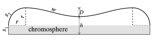
Figure 1: Magnetic loop used for the 1D radiative hydrodynamic simulations of the prominence oscillations. Note that the horizontal and the vertical sizes are not to scale.

Our simulations start from a thermal and force-balanced equilibrium state where the background heating is balanced by radiative loss and thermal conduction, and the plasma in the loop is quiescent. The simulations are divided into three steps: (1) Prominence formation: A prominence forms and grows near the center of the magnetic dip as chromospheric material is evaporated into the corona and condensates due to thermal instability after chromospheric heating is introduced near the footpoints of the loop; (2) Prominence relaxation: The prominence relaxes to a thermal and force-balanced equilibrium state as the localized heating is halted and the chromospheric evaporation ceases; (3) Prominence oscillation subjected to perturbations: The prominence starts to oscillate with a damping amplitude after perturbations are introduced. In step 1, which lasts for a time interval of $\Delta t_{1}$, the heating term $H(s)$ in Eq. (3) is composed of two terms, i.e., the steady background heating $H_{0}(s)$ and the localized chromospheric heating $H_{1}(s)$, which are expressed as follows:

$$H_{0}(s)=\cases{E_{0}\exp(-s/H_{m}),&$s<L/2$;\cr E_{0}\exp[-(L-s)/H_{m}],&$L/2\leqslant s<L$;\cr}$$ (5)

$$H_{1}(s)=\cases{E_{1},&$s\leqslant s_{tr}$;\cr E_{1}\exp[-(s-s_{tr})/\lambda],&$s_{tr}<s\leqslant L/2$;\cr E_{1}\exp[-(L-s_{tr}-s)/\lambda],&$L/2<s\leqslant L-s_{tr}$;\cr E_{1},&$s>L-s_{tr}$;\cr}$$ (6)

where the quiescent heating term $H_{0}$ is adopted to maintain the hot corona with the amplitude $E_{0}=3\times 10^{-4}$ ergs cm^-3 s^-1 and the scale-height $H_{m}=L/2$, and the localized heating term $H_{1}$ is adopted to generate chromospheric evaporation into the corona with the amplitude $E_{1}=10^{-2}$ ergs cm^-3 s^-1, the transition region height $s_{tr}=6$ Mm, and the scale height $\lambda=10$ Mm. The heating is taken to be symmetric in order to form a static prominence near the magnetic dip center, so that we can easily control the manner how the prominence is triggered to oscillate. Our methodology is different from Luna & Karpen (luna12 (2012)) who used asymmetric heating which spontaneously leads to the oscillation once the prominence is formed. In step 2, $H_{1}$ is switched off. Owing to the absence of the chromospheric evaporation, the gas pressure inside the magnetic loop drops down, so the compressed prominence expands until a new equilibrium is reached, which roughly takes less than 2.4 hr. In step 3, a perturbation is introduced to the prominence in order to trigger its oscillation. Note that $H_{0}$ remains throughout the simulations.

From the observational point of view, there might be two kinds of perturbations. The first one is an impulsive momentum injected to the magnetic loop as the magnetic reconnection near the footpoints rearranges the magnetic loop rapidly. The second is impulsive heating due to subflares (e.g., Jing et al. jing03 (2003), Vršnak et al. vrn07 (2007), Li & Zhang li12 (2012)) or microflares (Fang et al. fang06 (2006)) near the footpoints of the magnetic loop where a large amount of magnetic energy is impulsively released through magnetic reconnection. The gas pressure is greatly increased that could propel the prominence to oscillate along the dip-shaped field lines. In our 1D simulations, we separate the two effects to see their difference. In one case, a velocity perturbation with the following distribution is imposed to the prominence,

$$v(s)=\cases{0,&$s<s_{\rm pl}-\delta$;\cr v_{0}(s-s_{\rm pl}+\delta)/\delta,&$s_{\rm pl}-\delta\leqslant s\leqslant s_{\rm pl}$;\cr v_{0},&$s_{\rm pl}\leqslant s\leqslant s_{\rm pr}$;\cr v_{0}(-s+s_{\rm pr}+\delta)/\delta,&$s_{\rm pr}\leqslant s\leqslant s_{\rm pr}+\delta$;\cr 0,&$s>s_{\rm pr}$,\cr}$$ (7)

where $s_{\rm pl}$ and $s_{\rm pr}$ are the coordinates of the left and right boundaries of the prominence, $\delta=10$ is the buffer zone which allows that the perturbation velocity varies smoothly in space, and $v_{0}$ is the perturbation amplitude. In the other case, impulsive heating ($H_{2}$), as described as follows, is introduced near the right-hand footpoint of the magnetic loop,

$$H_{2}(s)=E_{2}\exp{\left[{-\frac{(s-s_{peak})^{2}}{s_{scale}^{2}}-\frac{(t-t_{peak})^{2}}{t_{scale}^{2}}}\right]},$$ (8)

where the heating spatial scale $s_{scale}=2.5$ Mm, the peak location $s_{peak}=245$ Mm, the heating timescale $t_{scale}=5$ min, and the peak time $t_{peak}=15$ min. The heating ramps up to the peak for 15 min and then fades down to 0.

As for the boundary conditions, all variables at the two footpoints of the magnetic loop are fixed, which is justified because the density in the low atmosphere is more than four orders of magnitude higher than that in the corona. The same approach has been adopted by Ofman & Wang (ofm02 (2002)) and Xia et al. (xia11 (2011)), assuming that the coronal dynamics has little effect on the low atmosphere. The approach was verified by Hood (hood86 (1986)) with the parameters being far from the marginal stability. The violation of the rigid wall conditions in certain cases was discussed by van der Linden et al. (van94 (1994)).

3 Effects of the perturbation type

In order to check how the two types of perturbations as described in §2 influence the characteristics of the prominence oscillations, we perform simulations of the oscillations which are excited by the two types of perturbations while keeping $\Delta t_{1}=7.2$ hr, $r=20$ Mm, $D=10$ Mm, and $L=260$ Mm.

In case A, the prominence oscillation is triggered by a velocity perturbation over the whole prominence body. With $v_{0}=-40$ km s^-1 (the minus means that the velocity is toward the left), the temporal evolution of the plasma temperature distribution along the magnetic loop is displayed in the left panel of Fig. 2. It is seen that in response to the perturbation, the prominence, signified by the low temperature, starts to oscillate around the equilibrium position. The oscillation amplitude decays with time. Fitting the trajectory of the mass center of the oscillating prominence with a decayed sine function

$$s=s_{0}+A_{0}\sin({2\pi\over P}t+\phi_{0})\exp{(-t/\tau)},$$ (9)

we find the initial amplitude $A_{0}=34.9$ Mm, the oscillation period $P=84.3$ min, and the damping timescale $\tau=272$ min. Assuming that the prominence thread has a cross-section area of $\sim 3.14\times 10^{14}$ cm² (Lin et al. lin05 (2005)), the initial kinetic energy of the oscillating prominence thread is estimated to be $\sim 7.2\times 10^{23}$ ergs. It is noted that the single decayed sine function, as used for fitting the H$\alpha$ observations (Jing et al. jing03 (2003); Vršnak et al. vrn07 (2007); Zhang et al. zhang12 (2012)), fits the simulated observations very well. On the contrary, a combination of Bessel function and an exponential decay function is necessary to fit the initial overtone in the simulations of Luna & Karpen (luna12 (2012)), which results from the continual mass accumulation.

In case B, the prominence oscillation is triggered by the impulsive heating which is deposited near the right leg of the magnetic loop in order to mimic a microflare near the prominence. To do that, an impulsive heating term $H_{2}(s)$ in Eq. (8) is added to the heating term $H$ in Eq. (3), where $s_{peak}=245$ Mm meaning the heating is concentrated at a height of 15 Mm above the right footpoint of the magnetic loop.

The right panel of Fig. 2 depicts the temporal evolution of the temperature distribution along the magnetic loop with $E_{2}=0.24$ ergs cm^-3 s^-1. With the typical cross-section area of a prominence thread being $\sim$3.14$\times$10¹⁴ cm², the corresponding total energy deposited into the single magnetic loop $E_{heating}$ is 1.8$\times 10^{25}$ ergs. This value is reasonable since observations indicate that the total energy of a microflare is 10²⁶–10²⁷ ergs or even more (e.g., Shimizu et al. shim02 (2002); Hannah et al. han08 (2008); Fang et al. fang10 (2010)), and several percent of the released energy goes into one prominence thread. From another point of view, under the framework of magnetic reconnection model for microflares, the magnetic energy release rate is estimated to be $B^{2}v_{in}/(4\pi L)$. With the magnetic field $B\sim 20$ G, the reconnection inflow speed $v_{in}$ being about 0.1 times the Alfvén speed which is about 1000 km s^-1 (Jiang et al. jia12 (2012)), and the spatial size $L=10\arcsec$, the energy release rate is estimated to be $\sim 0.88$ ergs cm^-3 s^-1, which is of the order adopted here. Fitting the trajectory of the oscillating prominence with the damped sine function as shown in Eq. (9) yields $A_{0}=35.8$ Mm, $P=84.3$ min, and $\tau=268$ min. The corresponding initial velocity is also -40 km s^-1. This indicates that a typical microflare near the leg of the magnetic loop hosting a prominence thread can excite the prominence longitudinal oscillations with an initial velocity of tens of km s^-1. The corresponding kinetic energy is only $\sim 7.2\times 10^{23}/1.8\times 10^{25}$, i.e., $\sim$4% of the deposited thermal energy. The remaining $\sim$96% of the energy deposit contributes to the heating of the chromosphere.

  

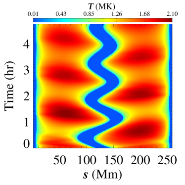
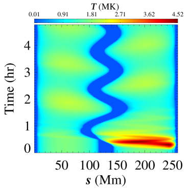
Figure 2: Comparison of the evolutions of the temperature of the loop between the two types of perturbations. The left panel corresponds to the case with velocity perturbations with $v_{0}=-40$ km s^-1 and the right panel to the case with localized heating perturbations with $E_{2}=0.24$ ergs cm^-3 s^-1.

4 Parameter survey

The results in §3 reveal that the oscillation period does not strongly depend on the two types of perturbations, i.e., impulsive momentum and localized heating at one footpoint used in our investigation. Note that we concentrate on the oscillation characteristics which follow the small transient/excitation phase, already obtained from simple decaying sinusoidal fitting. A small difference in the decay timescale exists between the two perturbation types. With the same initial velocity, the decay timescale is 4 minutes shorter in the case of impulsive heating than that in the case of impulsive momentum. However, the relative variation, 1.4%, is very small. Therefore, we can conclude that the oscillation is basically intrinsic and the characteristics of the oscillation depend on the prominence itself and the geometry of the magnetic loop in our case where there is no mass accumulation and the oscillations are excited by either impulsive momentum or localized heating. The prominence feature is only characterized by the thread length ($l$), and the geometry of the magnetic loop is characterized by $r$, $D$, and $w$ as depicted in Fig. 1. Among the three geometrical parameters, $h=s_{1}+r-D$ determines the height of the prominence, $D$ and $w$ determine the curvature of the magnetic dip. If other parameters are fixed, the length of the prominence is determined by the duration of the chromospheric evaporation in step 1, i.e., $\Delta t_{1}$, as described in §2. Besides, the decay timescale might vary with the perturbation amplitude, therefore another parameter is the initial perturbation velocity $v_{0}$. In this section, we perform a parameter survey to investigate how each individual one among the five parameters ($\Delta t_{1}$, $r$, $D$, $w$, and $v_{0}$) changes the oscillation period and the decay timescale. For each parameter, several cases with different values are simulated with other parameters fixed. In our simulations, we set $r=10$ Mm, $D=5$ Mm, $w=110$ Mm, and $v_{0}=-20$ km s^-1 when varying $\Delta t_{1}$. We set $\Delta t_{1}=7.16$ hr, $D=5$ Mm, $w=90$ Mm, and $v_{0}=-20$ km s^-1 when varying $r$. We set $\Delta t_{1}=7.16$ hr, $D=5$ Mm, $r=10$ Mm, and $v_{0}=-20$ km s^-1 when varying $w$. We set $\Delta t_{1}=7.16$ hr, $r=20$ Mm, $w=93.6$ Mm, and $v_{0}=-20$ km s^-1 when varying $D$. We set $\Delta t_{1}=7.16$ hr, $r=20$ Mm, $w=93.6$ Mm, and $D=10$ Mm when varying $v_{0}$. Since the oscillation characteristics are found nearly insensitive to the perturbation type, we use the velocity perturbation to excite the oscillations in the survey.

4.1 Length and mass of the prominence

After finishing the first two steps of the simulations as described in §2, we get a quasi-static prominence. The dependence of the prominence length $l$ on $\Delta t_{1}$, $h$, $D$, and $w$ is shown in the four panels of the upper row of Fig. 3. It can be seen that $l$, which fits into the scaling law $l\sim\Delta t_{1}^{0.70}$, increases with the duration of the heating time $\Delta t_{1}$. It is understandable since more chromospheric plasma is evaporated into the corona when $\Delta t_{1}$ increases. The length $l$ decreases with $h$ as $l\sim h^{-0.37}$, which is probably because it takes a longer time for the more tenuous corona to condensate as the height of the magnetic dip increases, and therefore the effective heating time is shorter. The length $l$ decreases with $D$ as $l\sim D^{-0.21}$, which can be understood as the prominence becomes more compressed as the magnetic dip becomes deeper. However, the length of the prominence does not vary considerably with $w$. Of course, $w$ should not be too small, otherwise thermal instability would not occur. The lengths of these simulated prominence threads are consistent with the reported values, i.e., tens of Mm (Lin et al. lin05 (2005)).

The dependence of the prominence mass $M$ on $\Delta t_{1}$, $h$, $D$, and $w$ is shown in the four panels of the lower row of Fig. 3. It can be seen that the dependence of $M$ on $\Delta t_{1}$, $h$, and $w$ is similar to $l$. Their difference is that $l$ decreases with $D$ whereas $M$ does not change with $D$, which means that the plasma number density (10¹⁰–10¹¹ cm^-3, and the corresponding density is 10^-14–10^-13 g cm^-3) is higher in the prominence with a deeper magnetic dip. A scaling law is obtained by fitting the data points, which is $M\sim\Delta t_{1}^{0.98}h^{-0.34}$.

It is noted that the above results are derived for a dipped magnetic loop filled via chromospheric evaporation with a limited lifetime, where the prominence thread can sustain in the corona. In the case of magnetic loops without a dip (e.g., Mendoza-Briceño et al. men05 (2005)) or with a shallow dip and asymmetric heating (e.g., Karpen et al. karp06 (2006)), condensations repetitively form, stream along the magnetic field, and ultimately disappear after falling back to the nearest footpoint. Therefore, the mass and length of the prominence evolve dynamically, without reaching an equilibrium value.

Figure 3: Scatter-plots of the total length $l$ (upper panels) and mass $M$ (lower panels) of the prominences at the end of relaxation step as functions of $\Delta t_{1}$, $h$, $D$, and $w$.

4.2 The oscillation period and decay timescale

As the velocity perturbation is introduced to the quasi-static prominence, the prominence starts to oscillate. Fitting the trajectory of the oscillating prominence with the damped sine function shown in Eq. (9), we get the oscillation period ($P$) and the decay timescale ($\tau$) for each case in the parameter survey.

The variations of $P$ along with the parameters $l$, $h$, $D$, $w$, and $v_{0}$ are shown in the upper row of Fig. 4. It is seen that $P$ increases slightly with $l$ and $v_{0}$, and decreases slightly with $h$. However, it increases seriously with $w$ and decreases with $D$. To fit the variations with a scaling law, we obtain $P\sim l^{0.16}h^{-0.05}D^{-0.54}w^{0.91}v_{0}^{0.05}$. Therefore, the period of prominence longitudinal oscillations relies dominantly on the geometry of the dip, especially its curvature. It is noted that the range of $P$ is in agreement with the reported values in previous studies (e.g., Jing et al. jing06 (2006)).

The variations of $\tau$ along with the five parameters are shown in the lower row of Fig. 4. It is seen that $\tau$ increases significantly with $l$ and $D$, and decreases with $w$ and $v_{0}$. It is noted that in the cases of $|v_{0}|=70$ and 80 km s^-1, part of the prominence mass drains down to the chromosphere, which is why the triangles in the lower-right panel of Fig. 4 do not follow the trend of the data points denoted by the diamonds where $|v_{0}|<70$ km s^-1. The decay timescale does not vary significantly with $h$. To fit the variations with a scaling law, we obtain $\tau\sim l^{1.63}h^{-0.18}D^{0.66}w^{-1.21}v_{0}^{-0.30}$, where the cases with prominence drainage are not included in the fitting. The values of $\tau$ are also in the same order of magnitude as the observed ones.

Figure 4: Scatter-plots of the period $P$ (upper panels) and damping time $\tau$ (lower panels) of the prominences in the oscillation step as functions of $l$, $h$, $D$, $w$, and $v_{0}$. The values of $P$ and $\tau$ in the cases $|v_{0}|=70$ and 80 km s^-1 that cause mass drainage at the footpoint of the coronal loop are marked with triangles in the right panels.

5 Discussions

5.1 Restoring force

For an oscillating phenomenon, the most important thing is the determination of the restoring force, which directly decides the oscillation period. In our 1D hydrodynamic simulations, the only forces exerted on the prominence are the gravity and the gas pressure gradient, both are restoring forces for the longitudinal oscillations. In order to compare their importance, we calculate the two forces in the case with $\Delta t_{1}=7.16$ hr, $v_{0}=-40$ km s^-1, $r=20$ Mm, $D=10$ Mm, and $w=93.6$ Mm. The two forces are calculated when the prominence is the furthest from the equilibrium position. Despite that the plasma in prominences is hundreds of times denser than the ambient corona, it is not an ideal rigid body. For oscillations with higher modes as studied by Luna et al. (2012a ), the pressure gradient changes rapidly along the prominence thread. For the fundamental-mode oscillations in this paper, the prominence oscillates as a whole and the pressure gradient changes slightly along the thread. Therefore, for simplicity, we compare the overall magnitude of the two forces by a simple calculation instead of as point-to-point one in the simulations. The integral of the gravity force is quantified between the two ends of the prominence, i.e., $F_{g}=\int_{left}^{right}\rho|g_{\parallel}|ds=\int_{left}^{right}\rho g_{\odot}\frac{\pi D}{2w}|\sin(\frac{\pi(s-L/2)}{w})|ds$, where a unit area is assumed for the cross section. The integral of pressure gradient force over the prominence is expressed as $F_{p}=\int_{left}^{right}|\partial p/\partial s|ds=|p_{right}-p_{left}|$. The left and right boundaries of the prominence are defined to be where the density drops to 7$\times 10^{-14}$ g cm^-3. Figure 5 displays the temporal evolution of the ratio $F_{g}/F_{p}$, from which it is seen that the gravitational force is generally $\sim$10 times larger than the gas pressure gradient force.

Figure 5: Temporal variation of $F_{g}/F_{p}$ when the displacement of the prominence reaches maximum during each half-cycle in the case of $r=20$ Mm and $D=10$ Mm. The velocity perturbation is -40 km s^-1.

Since the gravity is the dominant restoring force, the overall motion of the prominence can also be described for simplicity as

$$M\frac{d^{2}x}{dt^{2}}=Mg_{\parallel}=-Mg_{\odot}\frac{\pi D}{2w}\sin(\frac{\pi x}{w}),$$ (10)

where $x=s-L/2$ is the displacement of the prominence from the equilibrium position. It is not easy to solve this equation analytically. However, if the oscillation amplitude is much smaller than the half width of the whole magnetic dip ($w$), we get the approximation $\sin(\pi x/w)\approx\pi x/w$. So, the above equation is simplified to be

$$M\frac{d^{2}x}{dt^{2}}=-Mg_{\odot}\frac{\pi D}{2w}\frac{\pi x}{w},$$ (11)

with the solution $x=A_{0}\sin(\frac{2\pi}{P}t+\phi)$. The corresponding period is

$$P=\sqrt{\frac{8w^{2}}{g_{\odot}D}}.$$ (12)

Such a period can also be readily obtained if the prominence is taken in analogy to a pendulum whose period is

$$P=2\pi\sqrt{\frac{R}{g_{\odot}}},$$ (13)

where $R$ is the curvature radius of the dipped magnetic loop. With the shape of the loop being $y=D-D\cos(\pi x/2w)$, the curvature radius at the loop center is approximated to be $R=2w^{2}/(D\pi^{2})$. Substituting $R$ into Eq. (13), we get $P=\sqrt{8w^{2}/(g_{\odot}D)}$, the same as Eq. (12). Figure 6 compares the oscillation periods obtained from the hydrodynamic simulations (diamonds) and those estimated from Eq. (12) (solid line) when the two parameters, $D$ and $w$, are changed. It is revealed that Eq. (12) is a very good approximation for estimating the period of the prominence longitudinal oscillation. Of course, it should be kept in mind that the derivation of Eq. (12) is based on the assumption that the dipped magnetic loop has a sinusoidal shape. More generally, the oscillation period is related to the local curvature radius $R$ by the formula $P=2\pi\sqrt{R/g_{\odot}}$, as also demonstrated by Luna & Karpen (luna12 (2012)).

Recently, Luna et al. (2012a ) extended the theoretical analysis of longitudinal prominence oscillations by including the effect of the pressure gradient force. They found that the ultimate fundamental frequency of the oscillations is found from $\omega_{\rm fund}^{2}=\omega_{g}^{2}+\omega_{s}^{2}$, where $\omega_{g}$ and $\omega_{s}$ stand for the gravity-driven and pressure-driven frequencies, respectively. The ratio of the two frequencies $\omega_{g}^{2}/\omega_{s}^{2}=R_{\rm lim}/R$, where $R_{\rm lim}$ denotes the critical value of the curvature radius ($R$) of the magnetic dip. If $R\ll R_{lim}$, then gravity dominates over pressure in the restoring force of longitudinal oscillations. They pointed out that the reported values of the curvature are small compared with $R_{\rm lim}$, so that it is reasonable to ignore the effect of the pressure term in most cases. In our parameter survey, $R_{\rm lim}=0.175(L-l)l$ ranges from 760 to 2100 Mm and the ratio $R/R_{\rm lim}$ ranges from 0.1 to 0.5. Hence, their theoretical results of gravity being the main restoring force for the fundamental mode in this parameter range are thus confirmed by our simulations.

For a prominence above the solar limb, all the parameters in Eq. (12) can be roughly measured. Combined with the results in this paper, the comparison between simulations and observations in Zhang et al. (zhang12 (2012)) implies that Eq. (12) is a good approximation to estimate the oscillation period. For the prominence longitudinal oscillations on the solar disk, i.e., filament longitudinal oscillations, only the oscillation period can be unambiguously measured. Eq. (12) then provides a diagnostic tool for inferring the geometry of the dipped magnetic loop. Especially, when $w$ can be roughly estimated from force-free magnetic extrapolations, the depth of the dip, $D$, can be determined. At least, we can estimate the curvature radius of the dipped magnetic field, $R$, through Eq. (13). After the determination of $R$, Luna & Karpen (luna12 (2012)) further proposed an approximate method to estimate the magnetic field in the prominence.

Besides the dominant dependence on the geometric parameters, the oscillation period also weakly changes with the length and the height of the prominence, as well as with the initial velocity. These can be understood as follows: (1) Dependence on the prominence length: As the prominence thread is shorter, the ratio of the gas pressure gradient to the gravity would increase as indicated by our simulations, therefore, the gas pressure gradient would contribute to the restoring force, resulting in a shorter oscillation period; (2) Dependence on the prominence height: As seen from Fig. 3, with other parameters the same, a high prominence has a shorter length. Therefore, with the same reason as in (1), the oscillation period would be smaller; (3) Dependence on the initial velocity: Since $\sin(\pi x/w)$ is always smaller than $\pi x/w$ in Eq. (10), the nonlinear term would naturally lead to a long period as the oscillation amplitude increases.

Figure 6: Comparison of the periods of the prominence oscillations from simulations (diamonds) and theoretical analysis (solid line) as a function of the depth of the magnetic dip $D$ (left panel) and the width of the dip $w$ (right panel). Note that both axes are in logarithmic scale.

5.2 Damping mechanisms

If the energy dissipation terms such as the radiative cooling and the heat conduction are removed from Eq. (3), as we did in a test simulation, we found that the prominence oscillation does not damp at all. When the two non-adiabatic terms are kept, the prominence oscillation always damps. In order to see the importance of the two terms, we calculate the time integrations of radiative loss ($E_{\rm R}$) and thermal conduction ($E_{\rm C}$) of the whole system after subtracting the corresponding values when the prominence is static at the center of the dip. Here $E_{\rm R}$ and $E_{\rm C}$ are the integrals of the radiative and the conductive terms in the energy equation Eq. (3), where the integrals are taken in the whole corona above the two footpoints. The evolutions of the ratio ($E_{\rm R}/E_{\rm C}$) in the cases of $v_{0}=-40$, -50, and -60 km s^-1 are displayed in Fig. 7. It is seen that the ratio is always larger than unity. Especially in the early stage of the oscillation when the amplitude is still large, $E_{\rm R}$ is even one order of magnitude larger than $E_{\rm C}$. It is also revealed that as the initial velocity increases, $E_{\rm R}$ becomes more and more important in most of the lifetime of the oscillation. Our results support the conclusions of Terradas et al. (terr01 (2001, 2005)) that radiative loss is responsible for the damping of the slow mode of prominence oscillations in the dip-shaped magnetic configurations, which seems to be different from the case of slow-mode waves propagating in the coronal loops where heat conduction contributes more to the damping (De Moortel et al. 2002a ; 2002b ).

Figure 7: Temporal variations of $E_{\rm R}/E_{\rm C}$ in the oscillation step in the cases of $v_{0}=-40$, -50, and -60 km s^-1.

The role of the radiative cooling can be understood in a simple model as follows: Since there are two segments of the corona in the magnetic loop, as the prominence oscillates, one part would be attenuated and the other be compressed. Suppose that the total length of the coronal part of the magnetic loop is unity, which includes the part $x$, which is to the left of the prominence, and the other part $1-x$, which is to the right of the prominence. Hence, the densities of the corona on the two sides are proportional to $1/x$ and $1/(1-x)$, respectively. The total optically-thin radiative loss of the coronal part is proportional to $x^{-2}+(1-x)^{-2}$, which is the minimum when $x=0.5$, i.e., when the prominence is situated at the equilibrium position. Whenever the prominence deviates from the loop center, the cooling becomes larger, dissipating the kinetic energy of the oscillating prominence. The model is best illustrated by the relationship between the damping timescale ($\tau$) and the initial amplitude of the oscillation, i.e., $A_{0}$ in Eq. (9). As $A_{0}$ increases, one of the two coronal parts is more severely compressed, so the radiative cooling $x^{-2}+(1-x)^{-2}$ deviates further away from the minimum value, i.e., it becomes larger. As a result, the oscillation decays more rapidly.

Based on the sinusoidal function, $A_{0}\propto v_{0}P$. Substituting Eq. (12) into it, we get $A_{0}\propto v_{0}wD^{-1/2}$. With this, it is not difficult to understand the positive correlation between the decay timescale $\tau$ and $D$ and the negative correlation between $\tau$ and $w$ as revealed by the lower row of Fig. 4. Along this line of thought, the dependence of the decay timescale on the prominence length can be explained as follows: As the prominence thread is longer, the coronal part of the magnetic loop, which radiates out the thermal energy, is shorter. More importantly, the longer thread, with the same initial velocity, has a larger kinetic energy. Therefore, it takes a longer time for the compressed coronal part to radiate it out.

It is seen from the first six cases (i.e., $|v_{0}|$ from 10 km s^-1 to 60 km s^-1) in the lower-right panel of Fig. 4 that the decay timescale decreases with the initial perturbation velocity nearly linearly. However, when $v_{0}$ is larger than 70 km s^-1, part of the prominence would overpass the magnetic loop apex and drain down. The critical velocity for the prominence to reach the loop apex can be roughly estimated as $v_{criti}\sim\sqrt{2g_{\odot}D}=23\sqrt{D/{\rm Mm}}$ km s^-1. Therefore, the value of $v_{criti}$ is 73 km s^-1 in the case of $D=$10 Mm. As revealed from our simulations, even when $v_{0}$=-70 km s^-1, mass drainage already happens, although the amount of the drainage is much less than that in the case of $v_{0}=$-80 km s^-1. The temperature evolution along the loop in the case of $v_{0}=$-80 km s^-1 is presented in Fig. 8. It is seen that part of the prominence falls down to the left leg of loop, leading to the drainage of the prominence mass and kinetic energy as well, while the remaining part continues to oscillate along the dip. The oscillation period and the decay timescale in the cases with mass drainage are marked as triangles in Fig. 4. Their periods, $\sim$90.6 min, are slightly below the trend defined by other cases without mass drainage (diamonds), which is consistent with the weak positive correlation between $P$ and the prominence length $l$. However, the damping timescales are greatly reduced, compared to the trend defined by other cases without mass drainage as seen from the lower-right panel of Fig. 4. Such a result, namely that mass drainage would greatly reduce the decay timescale, might explain the mismatch between the simulation and the observation of the decay of a prominence oscillation reported in Zhang et al. (zhang12 (2012)).

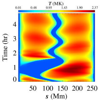
Figure 8: Temporal evolution of the temperature along the magnetic loop when the initial velocity perturbation is as large as $v_{0}=$-80 km s^-1. Note that the prominence overpasses the magnetic loop apex and drains down to the chromosphere at the left footpoint around $t=0.8$ hr.

6 Summary

In this paper, we carry out 1D hydrodynamic simulations of longitudinal prominence oscillations using the MPI-AMRVAC code, extending earlier numerical simulations of prominence formation (Xia et al. xia11 (2011)) and of prominence oscillations (Luna & Karpen luna12 (2012); Zhang et al. zhang12 (2012)). The simulations are divided into three steps: First, a prominence forms and grows near the center of the dip-shaped coronal loop due to chromospheric heating and the subsequent thermal instability. Then, it relaxes to a quiescent state after the chromospheric heating is switched off. Subjected to two kinds of perturbations that mimic subflares, the prominence starts to oscillate along the dip. Within the framework of the evaporation-condensation model, we obtained scaling-laws for the prominence length ($l$) and mass ($M$), which are expressed as $l\sim\Delta t_{1}^{0.70}h^{-0.37}D^{-0.21}$ and $M\sim\Delta t_{1}^{0.98}h^{-0.34}$, where $\Delta t_{1}$ is the time duration of the chromospheric heating and evaporation, $h$ is the prominence height, $D$ is the depth of the magnetic dip. It is found that $l$ is insensitive to the half length of the magnetic dip ($w$) once $w$ is large enough, say, 60 Mm; $M$ is insensitive to $D$ and $w$. Both transient heating at one leg of the loop and an impulsive velocity perturbation applied to the prominence as a whole are capable of driving a coherent oscillation along the dip. The oscillation properties are found insensitive to the perturbation type in the regimes studied. In the case of the transient heating, $\sim$4% of the deposited energy is converted into the kinetic energy of the prominence. The longitudinal oscillations are sustained mainly by the tangential component of gravity, except when the prominence is short and the gas pressure gradient becomes also important. Both simulations and linear analysis reveal that the period of oscillation ($P$) is 2$\pi\sqrt{R/g_{\odot}}$, where $R$ denotes the curvature radius of the dip, as also found by Luna & Karpen (luna12 (2012)). Other parameters, such as the length and the height of the prominence, as well as the perturbation velocity, also affect $P$, though slightly. The longitudinal oscillations damp in the presence of non-adiabatic effects, i.e., radiative loss and thermal conduction (Soler et al. sol09 (2009)), among which the radiative loss plays a leading role. With the parameter survey, we obtained a scaling-law for the decay timescale $\tau$, which is expressed as $\tau\sim l^{1.63}D^{0.66}w^{-1.21}v_{0}^{-0.30}$, where $v_{0}$ is the initial velocity perturbation. We also found that prominence mass drainage, once it happens, significantly reduces the decay timescale, which may explain the mismatching between the simulations and the observations disclosed by Zhang et al. (zhang12 (2012)).

It is worth mentioning the limitation of the applications of the above results. According to this paper, the mass of a prominence thread is insensitive to the depth $D$ and the width $w$ of the magnetic dip. This is based on the prominence formation directly via chromospheric evaporation with a fixed lifetime $\Delta t_{1}$. According to Xia et al. (xia11 (2011)), the prominence would grow via siphon flow even when the localized heating is switched off, though the growth speed is much slower. Recently, Luna et al. (2012a ) pointed out that the restoring force of the longitudinal oscillations depends on the depth of the magnetic dip. For shallow dips, gas pressure plays an important role, while gravity is the main factor for deep dips. Besides, Li & Zhang (li12 (2012)) suggested that magnetic tension may also contribute to the restoring force. As for the damping mechanisms, several other effects might be taken into account in the future simulations, such as the wave leakage and plasma viscosity (Ofman & Wang ofm02 (2002)). However, some will only be quantifiable in true multidimensional configurations, e.g. starting from the prominences formed in Xia et al. (xia11 (2011)).

- (1) Antiochos, S. K., MacNeice, P. J., & Spicer, D. S. 2000, ApJ, 536, 494
- (2) Antolin, P., Shibata, K., & Vissers, G. 2010, ApJ, 716, 154
- (3) Arregui, I., & Ballester, J. L. 2011, Space Sci. Rev., 158, 169
- (4) Arregui, I., Oliver, R., & Ballester, J. L. 2012, Liv. Rev. Solar Phys., 9, 2
- (5) Aulanier, G., DeVore, C. R., & Antiochos, S. K. 2006, ApJ, 646, 1349
- (6) Blokland, J. W. S., & Keppens, R. 2011, A&A, 532, A94
- (7) Blokland, J. W. S., & Keppens, R. 2011, A&A, 532, A93
- (8) Bocchialini, K., Baudin, F., Koutchmy, S., Pouget, G., & Solomon, J. 2011, A&A, 533, A96
- (9) Chen, P. F. 2011, Living Reviews in Solar Physics, 8, 1
- (10) Chen, P. F., Innes, D. E., & Solanki, S. K. 2008, A&A, 484, 487
- (11) Colgan, J., Abdallah, J., Jr., Sherrill, M. E., et al. 2008, ApJ, 689, 585
- (12) De Moortel, I., Ireland, J., Walsh, R. W., & Hood, A. W. 2002, Sol. Phys., 209, 61
- (13) De Moortel, I., Hood, A. W., Ireland, J., & Walsh, R. W. 2002, Sol. Phys., 209, 89
- (14) DeVore, C. R., & Antiochos, S. K. 2000, ApJ, 539, 954
- (15) Eto, S., Isobe, H., Narukage, N., et al. 2002, PASJ, 54, 481
- (16) Fang, C., Tang, Y.-H., & Xu, Z. 2006, Chinese J. Astron. Astrophys., 6, 597
- (17) Fang, C., Chen, P.-F., Jiang, R.-L., & Tang, Y.-H. 2010, Research in Astronomy and Astrophysics, 10, 83
- (18) Gilbert, H. R., Daou, A. G., Young, D., Tripathi, D., & Alexander, D. 2008, ApJ, 685, 629
- (19) Guo, Y., Schmieder, B., Démoulin, P., Wiegelmann, T., Aulanier, G., Török, T., & Bommier, V. 2010, ApJ, 714, 343
- (20) Hannah, I. G., Christe, S., Krucker, S., et al. 2008, ApJ, 677, 704
- (21) Hershaw, J., Foullon, C., Nakariakov, V. M., & Verwichte, E. 2011, A&A, 531, A53
- (22) Hood, A. W. 1986, Sol. Phys., 105, 307
- (23) Hyder, C. L. 1966, ZAp, 63, 78
- (24) Isobe, H., & Tripathi, D. 2006, A&A, 449, L17
- (25) Jiang, R.-L., Fang, C., & Chen, P.-F. 2012, ApJ, 751, 152
- (26) Jing, J., Lee, J., Spirock, T. J., & Wang, H. 2006, Sol. Phys., 236, 97
- (27) Jing, J., Lee, J., Spirock, T. J., Xu, Y., Wang, H., & Choe, G. S. 2003, ApJ, 584, L103
- (28) Karpen, J. T., & Antiochos, S. K. 2008, ApJ, 676, 658
- (29) Karpen, J. T., Antiochos, S. K., & Klimchuk, J. A. 2006, ApJ, 637, 531
- (30) Karpen, J. T., Tanner, S. E. M., Antiochos, S. K., & DeVore, C. R. 2005, ApJ, 635, 1319
- (31) Keppens, R., Meliani, Z., van Marle, A. J., et al. 2012, Journal of Computational Physics, 231, 718
- (32) Keppens, R., Nool, M., Tóth, G., & Goedbloed, J. P. 2003, Computer Physics Communications, 153, 317
- (33) Kippenhahn, R., & Schlüter, A. 1957, ZAp, 43, 36
- (34) Kleczek, J., & Kuperus, M. 1969, Sol. Phys., 6, 72
- (35) Kuperus, M., & Raadu, M. A. 1974, A&A, 31, 189
- (36) Labrosse, N., Heinzel, P., Vial, J.-C. et al. 2010, Space Sci. Rev., 151, 243
- (37) Li, T., & Zhang, J. 2012, ApJ, 760, L10
- (38) Lin, Y., Engvold, O., Rouppe van der Voort, L., Wiik, J. E.,& Berger, T. E. 2005, Sol. Phys., 226, 239
- (39) Luna, M., & Karpen, J. 2012, ApJ, 750, L1
- (40) Luna, M., Díaz, A. J., & Karpen, J. 2012a, ApJ, 757, 98
- (41) Luna, M., Karpen, J. T., & DeVore, C. R. 2012b, ApJ, 746, 30
- (42) Mackay, D. H., Karpen, J. T., Ballester, J. L., Schmieder, B., & Aulanier, G. 2010, Space Sci. Rev., 151, 333
- (43) Mendoza-Briceño, C. A., Sigalotti, L. D. G., & Erdélyi, R. 2005, ApJ, 624, 1080
- (44) Müller, D. A. N., Peter, H., & Hansteen, V. H. 2004, A&A, 424, 289
- (45) Ning, Z., Cao, W., Okamoto, T. J., Ichimoto, K., & Qu, Z. Q. 2009, A&A, 499, 595
- (46) Ofman, L., & Wang, T. 2002, ApJ, 580, L85
- (47) Okamoto, T. J., Tsuneta, S., Berger, T. E., et al. 2007, Science, 318, 1577
- (48) Schmieder, B., & Aulanier, G. 2012, EAS Publications Series, 55, 149
- (49) Shimizu, T., Shine, R. A., Title, A. M., Tarbell, T. D., & Frank, Z. 2002, ApJ, 574, 1074
- (50) Soler, R., Oliver, R., & Ballester, J. L. 2009, ApJ, 693, 1601
- (51) Su, Y., & van Ballegooijen, A. 2012, ApJ, 757, 168
- (52) Tandberg-Hanssen, E. 1995, Science, 269, 111
- (53) Terradas, J., Oliver, R., & Ballester, J. L. 2001, A&A, 378, 635
- (54) Terradas, J., Carbonell, M., Oliver, R., & Ballester, J. L. 2005, A&A, 434, 741
- (55) Tripathi, D., Isobe, H., & Jain, R. 2009, Space Sci. Rev., 149, 283
- (56) van der Linden, R. A. M., Hood, A. W., & Goedbloed, J. P. 1994, Sol. Phys., 154, 69
- (57) Vršnak, B., Veronig, A. M., Thalmann, J. K., & Žic, T. 2007, A&A, 471, 295
- (58) Xia, C., Chen, P. F., & Keppens, R. 2012, ApJ, 748, L26
- (59) Xia, C., Chen, P. F., Keppens, R., & van Marle, A. J. 2011, ApJ, 737, 27
- (60) Xu, Z., Lagg, A., Solanki, S., & Liu, Y. 2012, ApJ, 749, 138
- (61) Zhang, Q. M., Chen, P. F., Xia, C., & Keppens, R. 2012, A&A, 542, A52