The UK Infrared Telescope M 33 monitoring project. III. Feedback from dusty stellar winds in the central square kiloparsec

Abstract

We have conducted a near-infrared monitoring campaign at the UK InfraRed Telescope (UKIRT), of the Local Group spiral galaxy M 33 (Triangulum). The main aim was to identify stars in the very final stage of their evolution, and for which the luminosity is more directly related to the birth mass than the more numerous less-evolved giant stars that continue to increase in luminosity. In this third paper of the series, we measure the dust production and rates of mass loss by the pulsating Asymptotic Giant Branch (AGB) stars and red supergiants. To this aim, we combined our time-averaged near-IR photometry with the multi-epoch mid-IR photometry obtained with the Spitzer Space Telescope. The mass-loss rates are seen to increase with increasing strength of pulsation and with increasing bolometric luminosity. Low-mass stars lose most of their mass through stellar winds, but even super-AGB stars and red supergiants lose $\sim 40$% of their mass via a dusty stellar wind. More than three-quarters of the dust return is oxygenous. We construct a 2-D map of the mass-return rate, showing a radial decline but also local enhancements due to agglomerations of massive stars. We estimate a total mass-loss rate of 0.004–0.005 M_⊙ yr^-1 kpc^-2, increasing to $\sim 0.006$ M_⊙ yr^-1 kpc^-2 when accounting for eruptive mass loss (e.g., supernovæ); comparing this to the current star formation rate of $\sim 0.03$ M_⊙ yr^-1 kpc^-2 we conclude that star formation in the central region of M 33 can only be sustained if gas is accreted from further out in the disc or from circum-galactic regions.

1 Introduction

Galactic evolution is driven at the end-points of stellar evolution, where copious mass loss returns chemically-enriched and sometimes dusty matter back to the interstellar medium (ISM); the stellar winds of evolved stars and the violent deaths of the most massive stars also inject energy and momentum into the ISM, generating turbulence and galactic fountains when superbubbles pop as they reach the “surface” of the galactic disc. The evolved stars are also excellent tracers, not just of the feedback processes, but also of the underlying populations, that were formed from millions to billions of years prior to their appearance. The evolved phases of evolution generally represent the most luminous, and often the coolest, making evolved stars brilliant beacons at IR wavelengths, where it is also easier to see them deep inside galaxies as dust is more tranpsarent at those longer wavelengths than in the optical and ultraviolet where their main-sequence progenitors shine. The final stages of stellar evolution of stars with main-sequence masses up to $M\sim 30$ M_⊙ – Asymptotic Giant Branch (AGB) stars and red supergiants – are characterised by strong radial pulsations of the cool atmospheric layers, rendering them identifiable as long-period variables (LPVs) in photometric monitoring campaigns spanning months to years (e.g., Whitelock, Feast & Catchpole 1991; Wood 2000).

The Local Group galaxy Triangulum (Hodierna 1654) – hereafter referred to as M 33 (Messier 1771) – offers us a unique opportunity to study stellar populations, their history and their feedback across an entire spiral galaxy and in particular in its central regions, that in our own Milky Way are heavily obscured by the intervening dusty Disc (van Loon et al. 2003; Benjamin et al. 2005). Our viewing angle with respect to the M 33 disc is more favourable (56–$57^{\circ}$ – Zaritsky, Elston & Hill 1989; Deul & van der Hulst 1987) than that of the larger M 31 (Andromeda), whilst the distance to M 33 is not much different from that to M 31 ($\mu=24.9$ mag – Bonanos et al. 2006). Large populations of AGB stars have been identified in M 33 (Cioni et al. 2008), and red supergiants up to progenitor masses in excess of 20 M_⊙ (Drout, Massey & Meynet 2012). Many of them are dusty LPVs (McQuinn et al. 2007; Thompson et al. 2009), and these have been found also in the central parts of M 33 (Javadi, van Loon and Mirtorabi 2011a).

The main objectives of our project are described in Javadi, van Loon & Mirtorabi (2011c): to construct the mass function of LPVs and derive from this the star formation history in M 33; to correlate spatial distributions of the LPVs of different mass with galactic structures (spheroid, disc and spiral arm components); to measure the rate at which dust is produced and fed into the ISM; to establish correlations between the dust production rate, luminosity, and amplitude of an LPV; and to compare the in situ dust replenishment with the amount of pre-existing dust. Paper I in the series presented the photometric catalogue of stars in the inner square kpc (Javadi et al. 2011a), and Paper II presented the galactic structure and star formation history in the inner square kpc (Javadi, van Loon and Mirtorabi 2011b). This is Paper III, describing the mass-loss mechanism and dust production rate in the inner square kpc. Subsequent papers in the series will cover the extension to a nearly square degree area covering much of the M 33 optical disc.

2 The data and methods

To derive the mass-loss rates of the red giant variables we follow a two-step approach. First, we model the spectral energy distributions (SEDs) of near-IR variables for which mid-IR counterparts have been identified. We use these results to construct relations between the dust optical depth and bolometric corrections on the one hand, and near-IR colours on the other. Then, we apply those relations to the red giant variables for which no mid-IR counterpart was identified, to derive their mass-loss rates too.

2.1 The near-IR data

Images in the J, H and K_s bands were obtained with the United Kingdom InfraRed Telescope (UKIRT) with the UIST instrument, covering an area of approximately $4^{\prime}\times 4^{\prime}$ corresponding to a square kpc at the distance of M 33. Observations in the K_s band were made on about a dozen occasions over the period of 2003–2007. The data, point spread function (PSF) fitting photometry with DAOphot (Stetson 1987) and variability analysis are described in Paper I. The full, publicly available catalogue contains 18 398 stars; 812 of these were identified as variables on the basis of the near-IR photometry alone, most of them pulsating red giant stars (AGB stars and red supergiants).

2.2 The mid-IR data

Images in the 3.6, 4.5, 5.8 and 8 $\mu$m bands were obtained with the Spitzer Space Telescope with the IRAC instrument, on six occasions over the period of 2004–2006. We use the photometric catalogue of McQuinn et al. (2007), which is based on PSF fitting with DAOphot to the first five epochs and excludes the less sensitive 5.8 $\mu$m band. Thompson et al. (2009) have published a somewhat deeper catalogue in the 3.6 and 4.5 $\mu$m bands including the sixth epoch, but they have not made publicly available their photometry obtained at longer wavelengths and we therefore prefer working with the homogeneous catalogue of McQuinn et al. We cross-matched our near-IR catalogue to their catalogue (see Paper I for details) and found 523 matches in the 3.6 $\mu$m band, 471 at 4.5 $\mu$m and 107 at 8 $\mu$m (Fig. 1).

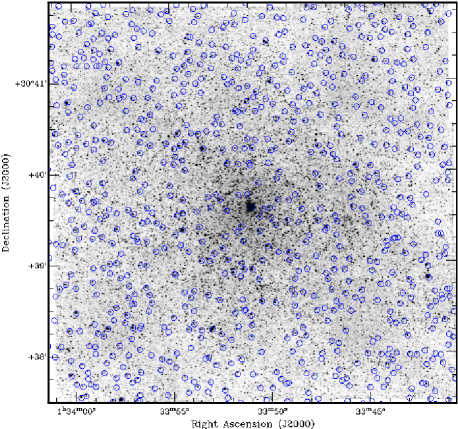
Figure 1: K_s band image of the central square kpc of M 33, overlain with the mid-IR sources from McQuinn et al. (2007).

We noticed (in Paper I) a discrepancy between the [3.6]–[4.5] colours and theoretical isochrones (from Marigo et al. 2008), with the faintest stars being abnormally blue. This is not apparent in the colour–magnitude diagram of M 33 as a whole (see McQuinn et al. 2007) and is most likely related to the specific challenges encountered in the crowded central regions of the galaxy (though strong absorption in the fundamental band of carbon monoxide can depress the 4.5 $\mu$m brightness, which is a challenge for models to predict accurately). The PSF of the mid-IR data has a full width at half maximum of $1\hbox to0.0pt{.\hss}^{\prime\prime}7$, which is more than twice as large as that of the near-IR data.

To gain an appreciation of the severity and effects of blending, we performed a simple simulation. First, we picked an individual K_s band frame and removed all detected stars from it with DAOphot/allstar (Stetson 1987). Next, we placed each of these stars back into the frame, at their original positions but using a $1\hbox to0.0pt{.\hss}^{\prime\prime}7$ PSF to mimic the appearance at 3.6 $\mu$m. We assumed that none of these stars have an infrared excess due to circumstellar dust, so their 3.6 $\mu$m counts can be derived from their K_s magnitude by applying a typical K_s–[3.6] colour of a few tenths of a magnitude (see figure 4 in van Loon, Marshall & Zijlstra 2005). Then, we used DAOphot/allstar and DAOmaster to detect and photomeasure the stars on this pseudo-3.6 $\mu$m frame.

Figure 2: Distributions of input magnitudes (solid histogram) and recovered magnitudes (dotted), derived from a pseudo-3.6 $\mu$m frame simulated on the basis of a real K_s band frame.

The distributions of input and recovered pseudo-3.6 $\mu$m magnitudes (Fig. 2) demonstrate that in the crowded central regions of M 33 the 3.6 $\mu$m photometry becomes severely incomplete for stars fainter than about magnitude 16, well before the K_s band data. Hence our simulation also accounts for unresolved emission at 3.6 $\mu$m from stars too faint to be detected individually. The recovery rate of stars brighter than magnitude 16 is very high.

Figure 3: Difference between input magnitude and recovered magnitude vs. input magnitude, derived from a pseudo-3.6 $\mu$m frame simulated on the basis of a real K_s band frame.

Stars brighter than magnitude 16 are recovered with reliable photometry, at an accuracy (much) better than 0.3 mag and showing no systematic offset (Fig. 3). Visual inspection of the few bright sources with large photometric discrepancies revealed that most of these stars were located near the very nucleus of M 33 or near the edge of the frame. Stars fainter than magnitude 16 start showing the effects of blending, leading to a reduction in the number of stars that are recovered (Fig. 2) and a systematic over-estimation of their brightness (Fig. 3).

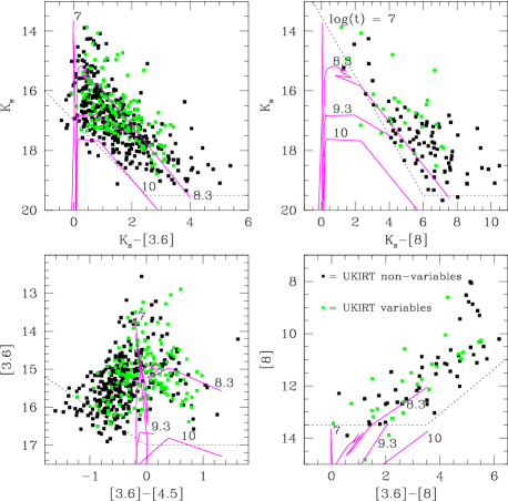
Figure 4: Near- and mid-IR colour–magnitude diagrams, with approximate detection boundaries (dotted lines) and overlain with theoretical isochrones from Marigo et al. (2008) for ages of $\log t=7$ ($t=10$ Myr), 8.3 (200 Myr), 9.3 (2 Gyr) and 10 (10 Gyr). UKIRT variable stars are plotted in green.

A useful number of stars (107) are detected at 8 $\mu$m because of excess emission from circumstellar dust, which allows derivation of their mass-loss rates. The stars form a branch of increasing mid-IR brightness with increasing near-/mid-IR colour (Fig. 4). The brightest mid-IR objects, $[8]<10$ mag, with very red colours, ($[3.6]-[8])\approx$ 5 mag, deviate from this main branch. These have not been identified by us as variable stars, and could be non-stellar in origin, for instance background galaxies or compact H ii regions within M 33. We will come back to these and other deviant sources at the end of Section 2.3 and in Section 3.1.

2.3 Modelling the spectral energy distributions

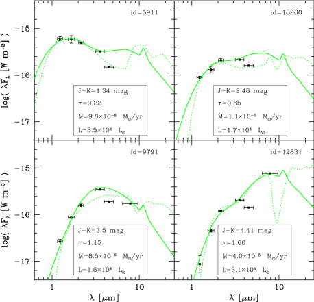
Figure 5: Near- and mid-IR photometry of examples of carbon stars in the centre of M 33, affected by various levels of mass loss. The horizontal “errorbars” on the data represent the width of the photometric passbands. The solid lines are the best matching SEDs modelled with dusty. The dotted lines are best matching fits using silicates, for comparison.

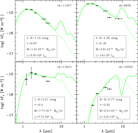
Figure 6: As Figure 5 but for examples of M-type stars. The dotted lines are best matching fits using amorphous carbon and silicon carbide, for comparison.

Table 1: UKIRT ID No. (Paper I), optical depth ($\tau$), luminosity ($L$) and mass-los rate ($\dot{M}$) determined by modelling of the SED with dusty. Note that there is a great deal of uncertainty in the classification into carbon and M-type stars. (The full table is available electronically.)

ID	$\tau$	$\log L$ (L⊙)	$\log\dot{M}$ (M⊙ yr-1)
carbon stars
629	0.07	4.45	$-5.52$
1003	0.03	4.42	$-6.43$
1590	0.06	4.42	$-5.95$
…	…	…	…
M-type stars
97	0.30	3.85	$-5.25$
901	0.20	4.15	$-4.93$
2323	0.10	3.92	$-5.62$
…	…	…	…

We modelled the SEDs of all UKIRT variable stars with measurements in at least two near-IR bands (K_s and J and/or H) and two mid-IR bands (3.6, 4.5 and/or 8 $\mu$m), with the publicly available dust radiative transfer code dusty (based on Ivezić & Elitzur 1997). Because of the scarcity of the photometry we fixed the input temperatures of the star and of the dust at the inner edge of the circumstellar envelope, at 3000 and 900 K, respectively. The density structure is assumed to follow from the analytical approximation for radiatively driven winds (Ivezić & Elitzur 1997). Based on the estimated birth mass of the star (see Paper II) we used amorphous carbon dust (Hanner 1988) and a small amount of silicon carbide (Pégourié 1988) for $1.5<M/{\rm M}_{\odot}<4$, and astronomical silicates (Draine & Lee 1984) for all other mass ranges, with a gas-to-dust mass ratio of $\psi=200$. The optical depth ($\tau$) was varied and the luminosity ($L$) was scaled until an acceptable match was obtained, which was decided by visual inspection. The optical depth and luminosity, and hence mass-loss rate ($\dot{M}$), were determined for 58 carbon stars and 35 M-type stars (Table 1); examples are presented in Figures 5 (carbon stars) and 6 (M-type stars).

Given the limited number of free parameters even a small number of data points constrain the model fit quite well. In all panels of Figs. 5 and 6 we not only show the best fit for the preferred dust species but also that for the alternative dust species. While it is not always possible to tell, on the basis of the fit, which species of dust is present, the preferred dust species often yields better fits and hardly ever yields worse fits. Our study spans several orders of magnitude in both mass-loss rate and luminosity, and the uncertainties resulting from the assumptions in the fitting procedures are thus relatively unimportant. A heavily dust-enshrouded pulsating giant star will still be fitted with a model with high optical depth regardless whether it employs carbonaceous or oxygenous dust. We do note, though, that often the 4.5-$\mu$m datum is anomalously faint compared to adjacent bands. This may be due to molecular absorption, which was not included in our SED modelling. The fundamental ro-vibrational band of CO at 4.6 $\mu$m can be strong especially in the extended atmospheres of pulsating red giant stars (cf. Nowotny et al. 2013). The 3-$\mu$m C₂H₂+HCN band is very strong in carbon stars, but it falls largely outside the IRAC 3.6-$\mu$m bandpass; the 3.8-$\mu$m C₂H₂ band, while strong in metal-poor carbon stars (van Loon et al. 2006, 2008), is not expected to be nearly as strong in the carbon stars in the central regions of M 33 that are of near-solar metallicity.

While this approach may seem crude (by necessity), we shall see that the results compare favourably with those obtained for similar populations of stars in the Magellanic Clouds.

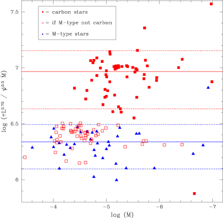
Figure 7: Combinations of the optical depth ($\tau$), luminosity ($L$), gas-to-dust mass ratio ($\psi$) and mass-loss rate ($\dot{M}$) obey scaling relations derived from the density structure of radiation-driven dust winds such that the plotted combination is constant to well within a factor two; the horizontal lines mark the median values (solid) and $\pm$ standard deviation (pairs of dotted lines). The open red squares show the results if the carbon stars are presumed to be oxygen-rich instead. The difference between carbon and M-type stars is due to the different optical properties of the dust grains.

The self-similarity of radiation-driven winds leads to scaling relations (Ivezić & Elitzur 1997), with the combination of $(\tau L^{3/4})/(\psi^{1/2}\dot{M})$ being approximately constant. Indeed it is, roughly, but with scatter ($\approx 0.2$ dex; Fig. 7) due to slight mis-matches between $\tau$ and $BC$ to the exact shape of the SED. The amount of scatter is rather modest, though, and suggests that the mass-loss rates for these stars are accurate to well within a factor two (cf. Srinivasan, Sargent & Meixner (2011); the luminosities for these stars are obtained with an accuracy of around 10–30 per cent). The offset between the carbon stars and M-type stars ($\approx 0.6$ dex $\equiv 4\times$) is expected as this is due primarily to the differences in opacity of the different dust species. Most – though not all – stars originally classified as carbon stars but fitted with silicates end up in a location slightly off-set from that of the M-type stars. This suggests that most of these stars are indeed different from the M-type stars and therefore quite possibly genuine carbon stars, but that some may have been misclassified and are in fact M type.

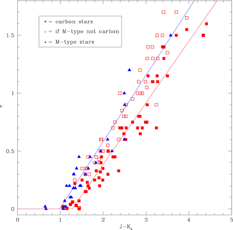
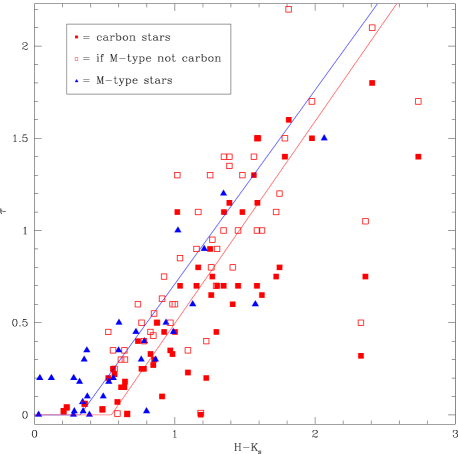
Figure 8: Relations between optical depth ($\tau$) and near-IR colours (top: J–K_s; bottom: H–K_s) for carbon stars (red squares) and M-type stars (blue triangles). The open red squares show the results if the carbon stars are presumed to be oxygen-rich instead. The red and blue lines are the adopted relations for carbon and M-type stars, respectively.

Table 2: Parameterisations of relations between optical depth ($\tau$) and near-IR colour ($C$) of the form $\tau=a+b\ C$ for $C\geq c$ mag (and $\tau=0$ for $C<c$ mag).

C	a	b	c		a	b	c
	carbon stars				M-type stars
J–Ks	$-$0.678	0.531	1.275		$-$0.5635	0.573	0.98
H–Ks	$-$0.601	1.096	0.548		$-$0.343	1.052	0.33

The measured optical depth correlates with near-IR colour – in particular the relation with J–K_s is tight and straight (Fig. 8). Because the relation between optical depth and colour directly reflects the optical properties of the dust species, carbon stars fitted with silicates land on the relationship for M-type stars fitted with silicates. Where J (and K_s) band photometry is available the optical depth is estimated by applying a parameterisation of the measured relation between $\tau$ and J–K_s; if only H (and K_s, but not J) band photometry is available then we apply a parameterisation of the relation between $\tau$ and H–K_s (see Table 2).

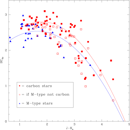
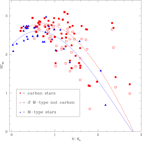
Figure 9: Relations between the bolometric correction to the K_s band ($BC_{\rm Ks}$) and near-IR colours (top: J–K_s; bottom: H–K_s) for carbon stars (red squares) and M-type stars (blue triangles). The open red squares show the results if the carbon stars are presumed to be oxygen-rich instead. The red and blue lines are the adopted relations for carbon and M-type stars, respectively.

Table 3: Parameterisations of relations between the bolometric correction to the K_s band ($BC_{\rm Ks}$) and near-IR colour ($C$) of the form $BC_{\rm Ks}=a+b\ C+c\ C^{2}+d\ C^{3}$.

C		a	b	c	d	e		a	b	c	d	e
		carbon stars						M-type stars
J–Ks		1.83	1.08	$-$0.3				1.84	0.84	$-$0.26
H–K${}_{\rm s}<e$		2.35	1.30	$-$0.98	0.08	5		2.24	1.27	$-$1.18	0.16	2.9
H–K${}_{\rm s}>e$		6.97	$-$2.52			5		4.42	$-$1.56			2.9

Likewise, the bolometric correction to the $K_{\rm s}$ band (BC_Ks) shows a dependency on near-IR colour (Fig. 9) – albeit with considerable scatter and with occasionally large deviations for H–K_s. This relation depends on the underlying star (its temperature), and the carbon stars fitted with silicates fall in between carbon stars fitted with carbonaceous dust and M-type stars fitted with silicates; this also drives the difference noted in Figure 7. Luminosities are estimated for the sample at large by applying a parametrisation of the relation between BC_Ks and J–K_s if $J$ is available and H–K_s if $H$ (but not $J$) is available (see Table 3). The scatter in Fig. 9 suggests that an accuracy in the luminosity is achieved of typically 30–50 per cent.

There exist pitfalls with this approach, which could lead to sources being erroneously assigned high luminosities and mass-loss rates. One such case comprises stars that have no J- or H-band counterpart because they are near to the edges of the survey area, or because they are heavily extincted by interstellar dust. Such sources would not normally have been identified as variable in our survey. We thus decided that we would ignore stars that have no J- or H-band magnitude and are not variable. This includes the few very bright mid-IR sources mentioned at the end of Section 2.2, that are likely non-stellar in origin. When they have no J- or H-band magnitude but are variable, inspection of the brightest such sources revealed no suspicion regarding their photometry and so for these stars we do assign a J-band magnitude viz. equal to a (conservative) detection limit of $J=21$ mag. Of just twelve such cases, the most extreme example is #11887: a large-amplitude variable ($A_{\rm Ks}=1.6$ mag), with luminosity $\log L=4.50$ and mass-loss rate $\log\dot{M}=-3.9$.

3 Results

3.1 Dust production and mass-loss rates as a function of stellar parameters

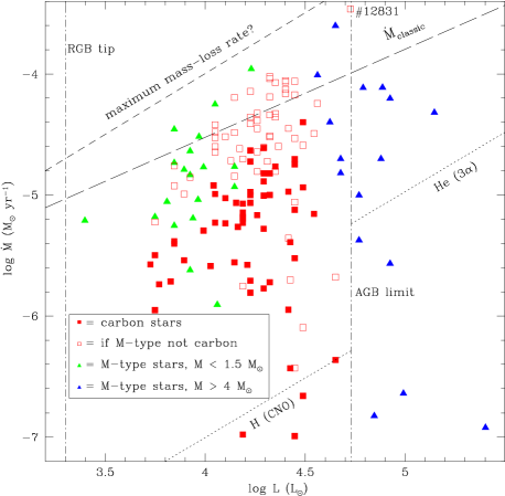
Figure 10: Mass-loss rate vs. luminosity, modelled with dusty, for low-mass AGB stars (green triangles), intermediate-mass AGB carbon stars (red squares) and massive AGB stars and red supergiants (blue triangles). The open red squares show the results if the carbon stars are presumed to be oxygen-rich instead. The tip luminosity of the RGB and classical limit of the most massive AGB stars (excluding the effects of Hot Bottom Burning) are indicated with vertical dash–dotted lines; the mass-consumption rates by shell hydrogen burning (CNO cycle) on the AGB and core helium burning (triple-$\alpha$ reaction) in red supergiants are indicated with diagonal dotted lines; and the limits to the mass-loss rate in dust-driven winds due to single scattering (classic) and multiple scattering (maximum?) are delineated with diagonal dashed lines (see van Loon et al. 1999). The highest rates are achieved by the most massive stars, but there is significant spread at all luminosities suggestive of evolutionary effects.

The mass-loss rate shows some dependence on luminosity (Fig. 10). Firstly, the highest rates are generally achieved by the most luminous, most massive stars, in agreement with earlier findings in the Magellanic Clouds (van Loon et al. 1999; Srinivasan et al. 2009). Except for a few more extreme examples that would probably have been missed in our survey, carbon stars in the Milky Way reach mass-loss rates of a few $\times 10^{-5}$ M_⊙ yr^-1 (Whitelock et al. 2006), whilst those in the Large Magellanic Cloud (LMC) reach $\dot{M}\sim 10^{-5}$ M_⊙ yr^-1 (Gullieuszik et al. 2012), i.e. comparable to the most extreme carbon stars in our M 33 sample. In the Solar Neighbourhood, M-type AGB stars reach similar mass-loss rates, a few $\times 10^{-5}$ M_⊙ yr^-1 (Jura & Kleinmann 1989), whilst M-type supergiants display rates between $10^{-7}<\dot{M}<10^{-4}$ M_⊙ yr^-1 with the majority in excess of a few $\times 10^{-6}$ M_⊙ yr^-1 (Jura & Kleinmann 1990), again both very similar to what we find in M 33.

Much of the spread in mass-loss rate at a given luminosity is likely to reflect stellar evolution (cf. van Loon et al. 1999, 2005a). The least luminous carbon stars ($\log L<4$) are probably not yet at the tip of their AGB because M-type AGB stars are found at the same luminosities but higher mass-loss rates – the latter are likely more evolved than the carbon stars; but these carbon stars are not expected to become M-type again (Marigo et al. 2008) so they must still evolve to higher luminosities before they end their AGB evolution. With $\dot{M}$ of a few $\times 10^{-6}$ M_⊙ yr^-1 they exhibit several times lower mass-loss rates than those near the tip of their AGB evolution (around $\log L\sim 4.3\equiv 20,000$ L_⊙) where they reach $\dot{M}$ in excess of $10^{-5}$ M_⊙ yr^-1. This suggests that the mass-loss rate increases as a star climbs the AGB.

Alternatively, the less luminous carbon stars with lower mass-loss rates may be in their inter-thermal pulse luminosity dip and/or the more luminous carbon stars with high mass-loss rates may just be experiencing the aftermath of a thermal pulse (Olofsson et al. 1990; Vassiliadis & Wood 1993; Mattsson, Höfner & Herwig 2007).

Fitting the stars that we originally classified as carbon stars with silicates generally yields higher mass-loss rates because of the lower specific opacity of silicates compared to amorphous carbon grains. One star, #12831 ($J-K_{\rm s}=4.4$ mag, $A_{\rm Ks}=0.63$ mag) has in this way become one of the more extremely mass-losing objects, with $\log\dot{M}=-3.5$ nine times higher than if fitted with silicates. The inferred birth mass would now be 6.7 M_⊙.

Evolution of red supergiants is mostly in terms of effective temperature ($T_{\rm eff}$) rather than luminosity. The dusty wind mass-loss rate depends sensitively on $T_{\rm eff}$ (van Loon et al. 2005a; cf. Bonanos et al. 2010); because red supergiants do not become as cool as massive AGB stars the highest rates achieved by red supergiants fall a little behind those achieved by the most extreme AGB stars considering that the red supergiants are more luminous (Fig. 10). Yet there is no luminosity gap in the stars with the highest mass-loss rates, confirming our earlier suggestion (Paper II) that super-AGB stars become dust-enshrouded. Super-AGB stars are strictly speaking red supergiants. However, the most massive AGB stars – i.e. those that will not ignite core carbon burning – experience Hot Bottom Burning (HBB; Iben & Renzini 1983); this not only prevents them from turning into carbon stars but also enhances their luminosity up and above the classical core-mass–luminosity relation (Boothroyd & Sackmann 1992). These stars may thus reach luminosities that exceed the classical AGB limit (indicated in Fig. 10), making it difficult to distinguish between an AGB star experiencing HBB and a super-AGB star or red supergiant. They may separate in $T_{\rm eff}$–$L$ diagrams (van Loon et al. 2005a) and thus also in $P$–$L$ diagrams (cf. Wood et al. 1992; Whitelock et al. 2003) and perhaps in $\dot{M}$–$L$ diagrams too. It is not very well established what is the maximum luminosity than can be reached under the influence of HBB, but it seems unlikely that it comprises much more than 50 per cent (0.2 dex). Depending on the timing of the ensuing supernova explosion, red supergiants might be found in the dust-enshrouded phase, or a preceding or following phase characterised by a thinner dust envelope. But if super-AGB stars explode they are likely to be dust-enshrouded, explaining explosions such as SN 2008S (Botticella et al. 2009).

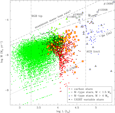
Figure 11: Mass-loss rate vs. luminosity. Massive, luminous M-type stars are depicted by blue triangles; AGB carbon stars by red squares; and low-mass M-type stars (at lower luminosities) by green triangles. Large yellow symbols identify the stars modelled with dusty; other UKIRT variable stars are identified by black squares. The most extreme mass-losing stars are labelled. The bottom panel shows the results if the carbon stars are presumed to be oxygen-rich instead.

The sample of stars that were modelled with dusty is not complete, and we therefore include in Figure 11 also the UKIRT variable stars for which no Spitzer photometry is available as well as non-variable stars. We note the most extreme datum in this graph, #13093, at $\log L=5.46$ and $\log\dot{M}=-3.0$. With $K_{\rm s}=16.96$ mag and $J-K_{\rm s}=5.35$ mag it is consistent with being a heavily-reddened $\simeq 14$ M_⊙ supergiant; we also identified it as a large-amplitude variable ($A_{\rm Ks}=1.05$ mag). Our K_s-band image shows a point source unaffected by crowding. No Spitzer photometry is available, neither from McQuinn et al. (2007) nor Thompson et al. (2009). Inspection of the IRAC images (3.6, 4.5, 5.8 and 8 $\mu$m) from the Spitzer archive, however, clearly reveals the source, adding credence to it being an extremely dusty evolved star. It sits next to an extended area of mid-IR emission, though, which may explain why it was not measured. It is almost twice as bright at 8 $\mu$m as the highest mass-losing UKIRT variable that we modelled with dusty (#15552), broadly in line with the factor 2.5 difference in their mass-loss rates.

On the other hand, the star with the next-highest mass-loss rate, #12208 ($\log L=5.04$, $\log\dot{M}=-3.6$) is more suspicious. With $K_{\rm s}=15.3$ mag it is bright, and with $J-K_{\rm s}=3.4$ mag it is red, but its estimated K_s-band amplitude is moderate ($A_{\rm Ks}=0.35$ mag). It is the brightest UKIRT variable in this central region of M 33 at 8 $\mu$m, by far (see Fig. 4). While it appears unresolved on the 8-$\mu$m image it sits on top of more complex emission, within $6^{\prime\prime}$ of a catalogued molecular cloud (Bolatto et al. 2008) and a supernova remnant (Gordon et al. 1999); this suggests it might be a young stellar object or even an ultra-compact H ii region.

A third object worth noting is the candidate $\eta$ Carinæ analogue M 33-8 (Khan, Stanek & Kochanek 2012). It is the only such object in their list of nine in M 33 that (just) falls within our UIST/UFTI survey. They combined optical photometry with 2MASS near-IR and Spitzer mid-IR data, to derive the spectral energy distribution and luminosity. They show a Hubble Space Telescope image in the visual dominated by a single source surrounded by a clustering of fainter stars. Our UFTI image reveals the dominant source is in fact a duplet in the K_s band, which would appear unresolved in the 2MASS image. The UIST catalogue lists them as #18469, with $K_{\rm s}=17.75$ mag, and #18441, with $K_{\rm s}=17.89$ mag. This compares well with the I-band magnitude (0.8 $\mu$m) listed in Khan et al. (2012) of $I=17.68$ mag. We estimate luminosities of $\log L=3.88$ and 3.68, respectively; i.e. together they fall well short of accounting for the integrated IR luminosity of $\log L_{\rm IR}=5.56$ derived by Khan et al. The latter must include significant contributions from other sources, especially as it includes the 24-$\mu$m Spitzer emission which has an angular resolution of only $6^{\prime\prime}$. We derive mass-loss rates of $\log\dot{M}=-5.2$ and $-5.1$ for #18469 and #18441, respectively; substantial, but not extreme.

Close pairs of infrared-bright stars are not unique. For instance, #19002 is an unresolved blend of two roughly equally-bright stars. We assigned a luminosity of $\log L=4.56$ and $\log\dot{M}=-3.8$ to the blended object; certainly at least one of the two stars is very dusty.

Figure 12: Mass-loss rate vs. K_s-band amplitude. Top: stars modelled with dusty – the open red squares show the results if the carbon stars are presumed to be oxygen-rich instead; bottom: all UKIRT variable stars, where large yellow symbols identify the stars modelled with dusty.

The mass-loss rate increases with increasing K_s-band amplitude (Fig. 12). The correlation is quite clear in spite of the relative inaccuracy of the amplitudes (determined from sparsely sampled lightcurves; see Paper I). The correlation is consistent with a rôle for stellar pulsation in driving the winds from cool stars; it also confirms that, whilst the relative amplitudes (expressed in magnitudes) are smaller for more luminous stars (the M-type stars with $M>4$ M_⊙ are the most luminous, those with $M<1.5$ M_⊙ are generally the least luminous), for the same amplitude the mass-loss rates are higher for more luminous stars: mass loss is more directly related to the absolute amplitude (expressed in luminosity units) (van Loon et al. 2008). The K_s band is relatively insensitive to variations in stellar temperature, circumstellar extinction and dust emission as it is near the peak of the stellar SED and in between the strong attenuation by dust at shorter wavelengths and its emission at longer wavelengths – hence also the preference for expressing bolometric corrections in relation to the K or K_s band. However, it is important, but difficult in practice, to separate the effects of pulsation and temperature on mass loss, as both the pulsation strengthens and the temperature decreases as the star ascends the RGB, AGB or red supergiant branch (see Whitelock, Feast & Pottasch 1987). The carbon stars confirm this picture in the sense that their amplitudes are intermediate between the more and less luminous M-type stars, but their mass-loss rates seem a little lower. As expected, the mass-loss rates of presumed carbon stars when fitted with silicates fall in between those of low-mass and higher-mass M-type stars. This fact neither confirms nor refutes their carbon star nature.

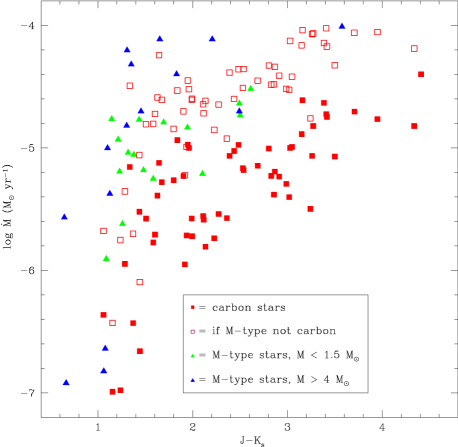
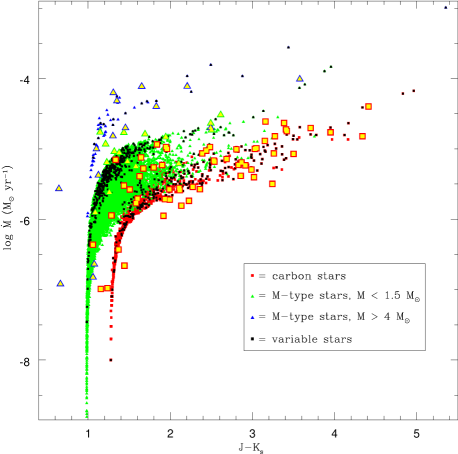
Figure 13: Mass-loss rate vs. J–K_s colour. Top: stars modelled with dusty – the open red squares show the results if the carbon stars are presumed to be oxygen-rich instead; bottom: all stars, where large yellow symbols identify the stars modelled with dusty and little black symbols identify the remaining UKIRT variable stars.

Mass-loss rates have often been correlated with infrared colour, to provide a simple recipe for converting infrared colours to mass-loss rates; however, these methods depend on the star’s luminosity as well as the dust properties (see van Loon 2007 for a review). Figure 13 exemplifies this once more: the carbon stars become easily reddened by their dust but that does not necessarily imply as high a mass-loss rate as a less reddened M-type star. Likewise, among stars with similar dust the less luminous stars are more readily reddened than more luminous ones (van Loon et al. 1999). Thus, care must be taken when converting an infrared colour into a mass-loss rate. The carbon stars’ luminosities are intermediate between those of the low-mass and higher-mass M-type stars, and indeed their mass-loss rates fall in between those groups’ mass-loss rates if also the presumed carbon stars are fitted with silicates.

3.2 Feedback into the interstellar medium

Assessments of the integrated mass loss (or dust production) from a stellar population are fraught with uncertainties. In small populations, stochastic effects are caused by very small numbers of stars which may dominate the budget (van Loon et al. 2005b; McDonald et al. 2009), but it is also difficult to accurately account for the many stars that each contribute little. Most red giants undergo mild mass loss and their circumstellar envelopes are not very dusty; photometric tracers of this mass loss and dust will be affected by photometric uncertainties and scatter in interstellar reddening, as well as uncertainties in the underlying photospheric spectral energy distribution (cf. McDonald, Zijlstra & Boyer 2012). Interstellar reddening towards the central region of M 33 is modest (see Paper I); whilst it is negligible for the dustiest stars it may lead to an over-estimate of the amount of dust produced by stars with little mass loss. Photometric scatter will also cause some stars to appear to have more dust than they really do, but equally cause the opposite effect in others. As this is of a purely statistical nature we can try to compensate for it by considering the distribution of stars over negative values for the optical depth as one would have derived them from the near-IR colour relation (Fig. 14, top). A similar distribution of erroneous optical depth values would extent towards positive values, and this distribution can be subtracted to yield the true distribution over optical depth (Fig. 14, bottom).

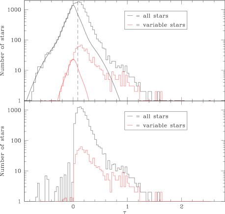
Figure 14: Top: Distribution of stars over optical depth, $\tau$, and bottom: after subtracting a multi-Gaussian fit to the negative values of $\tau$ which was centered at $\tau=0$. The UKIRT variables are plotted also separately, in red. The vertical dashed line marks the peak of the distribution of all stars.

The fraction of stars that were identified to be variable increases with increasing optical depth, to about unity for the most obscured specimens (Fig. 14). This is encouraging, suggesting that the dustiest stars produced most of that dust themselves. We cannot be certain, however, that the dust inferred for the non-variables and/or less obscured stars was all produced by themselves.

Because the mass-loss and dust-loss rate is derived from the optical depth via scaling with the luminosity, correcting the mass return is not straightforward. This correction can be applied statistically in two ways: (1) by reducing the contribution from each star by a factor $f/f_{0}$ where $f_{0}$ and $f$ are the distributions before and after correcting for the symmetric distribution around $\tau=0$, where $f/f_{0}\equiv 0$ for $\tau<0$; or (2) by including all stars including those with $\tau<0$, and assigning negative mass-loss rates to the latter. The problem with the second method is that some stars with very negative values and/or very high luminosities could make a large difference to the end result, whereas in the first method the correction is “smoother”. On the other hand, the second method accounts, to some extent, for variations of the correction factor with luminosity should such dependence exist. In what follows we have adopted the second method.

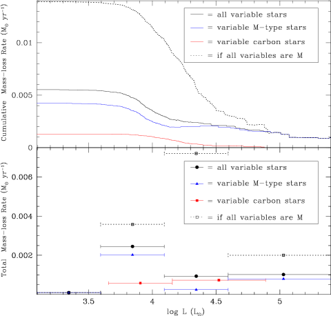
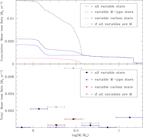
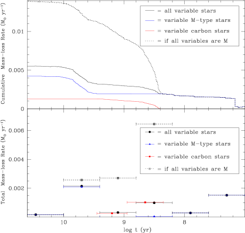
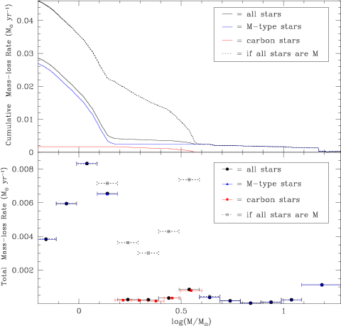
Figure 15: Mass-loss rate vs. luminosity (top left), age (bottom left) and birth mass (top right) for the UKIRT variable stars, and vs. birth mass for all stars including non-variable stars (bottom right). The top panels show the cumulative distribution (integrated from the right); the bottom panels show binned contributions. Distinction is made between likely carbon stars (red) and M-type stars (blue).

Hence we obtain the binned and cumulative mass-loss rate distributions depicted in figure 15. We concentrate on the mass-loss rates of the UKIRT variable stars, as these are believed to contribute the majority of the mass loss, but we also show the result including the non-variable stars – which are dominated by the low-mass red giants. The latter are numerous and therefore appear to contribute several times as much as the intermediate-mass AGB stars and higher-mass red supergiants, but it must be remembered that interstellar dust will be more often the cause of their generally modest reddening and so that result must be regarded as a firm upper limit to the mass return, of $<0.028$ M_⊙ yr^-1 (or $<0.046$ M_⊙ yr^-1 if all carbon stars are actually M-type stars). The true mass-return rate must be closer to that derived from the UKIRT variable stars, $\approx 0.0055$ M_⊙ yr^-1 (or $0.0139$ M_⊙ yr^-1 if all carbon stars are actually M-type stars). Accepting that some of the mass loss might have been missed – as not all variable stars may have been recognised in our survey – we could conceive a total mass-return rate of $\sim 0.006$–0.01 M_⊙ yr^-1 (up to $\sim 0.02$ M_⊙ yr^-1 if a large fraction of the carbon stars are actually M-type stars). Given the assumptions and uncertainties inherent to the mass-loss determinations we could hardly claim a higher degree of accuracy.

That said, low-mass M-type AGB stars appear to make a similar contribution to the mass return in the central regions of M 33 as all more massive stars combined. Among the latter, the massive carbon stars and red supergiants make similar contributions, while the low-mass carbon stars and massive AGB stars contribute less. As a result, the present-day mass-return arises mainly from stars formed in one of three major episodes: $t<40$ Myr ago ($\log t<7.6$), $t\sim 0.2$–1 Gyr ago ($\log t\sim 8.6$) and $t\sim 3$–10 Gyr ago ($\log t\sim 9.7$). This mainly reflects the star formation history (Paper II). The contribution from the intermediate-age population, formed $t\sim 0.2$–1 Gyr ago, is larger if the presumed carbon stars are actually mostly M-type stars, in which case they account for about half of the total mass return.

It is worthy of note that carbon grains make up $<23$% of the present-day dust-mass return, i.e. the interstellar dust is predominantly oxygen-rich. This fraction becomes even smaller if the population of carbon stars was overestimated.

The radial profile of the mass return rate (Fig. 16, in terms of surface density deprojected onto the galaxy plane – see Paper II) is flat within the inner $r<0.5$ kpc for the carbon stars. There appears to be a clear radial gradient for the M-type stars, with the mass return greatest within the central few hundred pc, but large deviations occur around $r\sim 0.3$–0.4 kpc. A more complete picture is obtained from the full 2-D map of mass return (Fig. 17, not deprojected), where a smooth level of gas and dust injection underlies dramatic local enhancements due to the concentration of red supergiants (and super-AGB stars) near to their sites of formation in discrete molecular cloud complexes. One of these includes #13093 and #12208, the supergiants with the highest mass-loss rates (see Section 3.1). For comparison we show a Spitzer composite in the left panel of figure 17 – note the bright source at ($1^{\rm h}34^{\rm m}00^{\rm s}$, $+30^{\circ}40^{\prime}47^{\prime\prime}$): this is M 33-8 (Kahn et al. 2012; see Section 3.1). The spatial distribution of mass return does not change markedly if the carbon stars turn out to be mostly M-type stars.

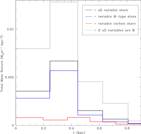
Figure 16: Radial distribution of mass-return-rate surface density over the central region of M 33.

4 Discussion and conclusions

If we believe the model predictions for the duration of the pulsation phase ($\delta t$, see table 2 in Paper II and Marigo et al. 2008) then we can calculate the mass lost during the pulsation phase as a fraction of the birth mass if we sample this phase both randomly and sufficiently:

$$\eta=\frac{\sum_{i=1}^{N}{\left(\dot{M}_{i}\times(\delta t)_{i}\right)}}{\sum_{i=1}^{N}{M_{i}}}.$$ (1)

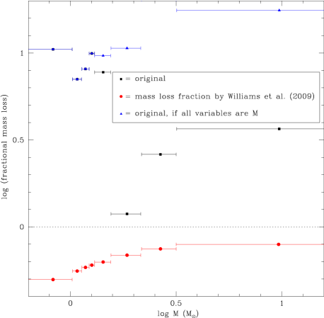
Figure 18: Top: ratio of the mass lost during the pulsational instability phase of stellar evolution, to the birth mass ($M$), i.e. the fraction of mass lost in the form of a dusty stellar wind. The dotted horizontal line marks the fiducial case where the star expels all of its mass. For comparison we also plot the fractional mass loss derived from the initial–final mass relation determined by Williams et al. (2009). Bottom: ratio of our derived fractional mass loss to that derived from the initial–final mass relation.

Obviously, this ratio should be less than unity. It is therefore somewhat disconcerting to find that this is not the case (Fig. 18), though it does lend support to our belief that the non-variable stars cannot contribute much to the total mass-loss budget, or it would seriously aggravate the situation. The integrated mass-loss along the evolution of low- and intermediate-mass stars is strongly constrained by the initial–final mass relation determined from white dwarfs in stellar clusters. The ratio of our values to those derived from the initial–final mass relation from Williams, Bolte & Koester (2009) varies between $<2$ and $\sim 20$. For massive stars the situation is more uncertain; while most of them (at the lower mass end) will leave behind a neutron star (of order a tenth of their birth mass) it is unclear how much mass is lost as a red supergiant, as a blue supergiant, and during the supernova explosion (see, e.g., Ekström et al. 2012). But what causes the discrepancy? Have the mass-loss rates been over-estimated? Or is the pulsation duration in error?

If the pulsation duration was over-estimated, then the star formation rate would have been under-estimated. At the time, we compared our estimate of the recent star formation rate, $\psi\approx 0.004$–0.007 M_⊙ yr^-1 kpc^-2, with work by Wilson, Scoville & Rice (1991) who had derived $\psi\sim 0.01$ M_⊙ yr^-1 kpc^-2. We were satisfied that, within the inherent uncertainties, these two estimates were consistent. In light of the above discrepancy between birth mass and lost mass, though, we now revisit these estimates:

• It is reasonable to assume that star formation occurs within the gas-rich disc, and so the recent star formation rate ought to be deprojected onto the galaxy’s plane. This depresses the rate by a factor $\cos i$ where $i$ is the angle of inclination of the normal to the M 33 disc with respect to the line-of-sight, for which we take $i=56^{\circ}$ (Zaritsky et al. 1989). The fact that the survey area is square but the position angle is $PA=23^{\circ}$ matters, but not a lot. So our estimate for the recent star formation rate becomes $\psi\approx 0.003$ M_⊙ yr^-1 kpc^-2.

• Several other groups have estimated star formation rates for the central region of M 33 (as part of larger surveys), from H$\alpha$ emission or the luminosity in the far-ultraviolet or far-infrared (Hippelein et al. 2003; Engargiola et al. 2003; Heyer et al. 2004; Gardan et al. 2007; Boissier et al. 2007; Verley et al. 2009). Kang et al. (2012) have summarised these works and they determine $\psi\sim 0.02$ M_⊙ yr^-1 kpc^-2 within the central square kpc of M 33, but possibly as much as 0.03–0.04 M_⊙ yr^-1 kpc^-2 (Heyer et al. 2004). This is $\sim 10$ times higher than our estimate.

If we shorten the pulsation duration (as used in Paper II) by this factor, then the fractional mass-loss of stars with masses $M>4$ M_⊙ ($\log M>0.6$) becomes $\eta\sim 0.4$. This reconciles the estimated mass-loss rates and star formation rates, given that some additional mass will be lost by the most massive stars as blue supergiants and supernovæ.

       

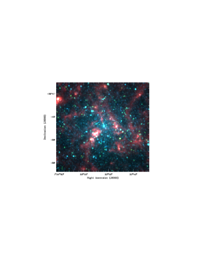
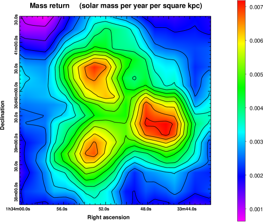
Figure 17: Left: Spitzer composite image of IRAC bands 1, 2 and 4 at respectively 3.6 $\mu$m (blue), 4.5 $\mu$m (green) and 8 $\mu$m (red); Right: map of mass-return-rate surface density over the central region of M 33.

Now that we have regained some confidence in the estimated values of the star formation rate and mass-return rate, we can consider the balance between the ISM depletion and replenishment. Kang et al. (2012) estimated an ISM depletion timescale of $M_{\rm ISM}/\psi\approx 0.3$ Gyr. But this does not take into account the continuous mass return by evolved stars, which would lengthen the depletion timescale. Our estimated mass-return rate (after deprojection) of $\dot{M}_{\rm return}\sim 0.004$–0.005 M_⊙ yr^-1 kpc^-2 (up to 0.01 M_⊙ yr^-1 kpc^-2 if all carbon stars are actually M-type stars) is more than our initially estimated recent star formation rate of $\psi\sim 0.003$ M_⊙ yr^-1 kpc^-2, but lower than the star formation rate estimated by other groups. We have just argued that our estimate of the star formation rate needs to be scaled up by a factor $\sim 10$, which would mean that the mass-return rate falls short of supplying the fuel for continued star formation by a factor 6 or 7 (or 3, if all carbon stars are actually M-type stars). The naive estimate of the depletion timescale of 0.3 Gyr would not change by more than 17% as a result of this mass return – and by at most 50% if all carbon stars turn out to be M-type stars.

However, additional mass is returned by supernovæ, hot massive-star winds, luminous blue variable eruptions, et cetera. Most of these contributions come from massive stars, which contribute about one third to the mass returned through dusty stellar winds (see Fig. 15, top right panel). Their fractional mass-loss (after correction for the shorter pulsation duration) is $\sim 40$%, i.e. they could at most contribute $\sim 2$ times as much as estimated here (accounting also for stellar remnants being left behind), which would increase the total mass-return rate (across all stellar masses) from $\sim 0.004$–0.005 to $\sim 0.006$ M_⊙ yr^-1 kpc^-2. Note that the contribution from low-mass stars is already fully accounted for by the dusty stellar winds. Thus, the above conclusion does not change, namely that the rate at which the ISM is replenished by stellar mass loss falls short by a factor $\sim 5$ to sustain star formation at the current rate. This conclusion does not change if all carbon stars turn out to be M-type stars, though the discrepancy is reduced to a factor $\sim 3$. For star formation to continue beyond the next few hundred Myr gas must flow into the central regions of M 33, either through a viscous disc or via cooling flows from the circum-galactic medium.

The mass return is not uniform across the central square kpc, so locally the above conclusions might not be accurate. The mass return by low-mass stars and carbon stars is fairly uniform across the area, with a slight radial gradient. But there are three areas at $r\sim 0.3$–0.4 kpc from the centre where the mass-return rate is much higher due to the contribution of several massive, very dusty stars. This could feed – and chemically enrich – enduring or new star formation in those areas on timescales of a couple of $10^{7}$ yr.

In Paper II we had found that the star formation rate peaks within the central $r<0.2$ kpc. The very centre of M 33, while characterised by high levels of mass return is not where the ISM is replenished at the highest rate. However, if gas from the dense regions at $r\sim 0.3$–0.4 kpc can be accreted into the nucleus of M 33 then this could be a mechanism for star formation to occur even within the nuclear star cluster. Indeed, Tosaki et al. (2011) find the molecular gas peaks at $r\sim 0.1$ kpc from the centre, and this could have been supplied at somewhat greater distances before being channeled towards the nucleus. They find another peak at $r\sim 0.6$ kpc which is at the edge of our survey area. The offsets of the peaks in the dense ISM with respect to the peaks in mass return (and star formation) suggest that, globally, there is a delay as well as a migration between the epochs and sites of intense mass return, accumulation of dense ISM, and star formation.

References

- [Benjamin et al.(2005)] Benjamin R. A., et al., 2005, ApJ, 630, L149
- [Boissier et al.(2007)] Boissier S., et al., 2007, ApJS, 173, 524
- [Bolatto et al.(2008)] Bolatto A. D., Leroy A. K., Rosolowsky E., Walter F., Blitz L., 2008, ApJ, 686, 948
- [Bonanos et al.(2006)] Bonanos A. Z. et al., 2006, ApJ, 652, 313
- [Bonanos et al.(2010)] Bonanos A. C., et al., 2010, AJ, 140, 416
- [Boothroyd & Sackmann (1992)] Boothroyd A. I., Sackmann I.-J., 1992, ApJ, 393, L21
- [Botticella et al.(2009)] Botticella M. T. et al., 2009, MNRAS, 398, 1041
- [Cioni et al.(2008)] Cioni M.-R. L., et al., 2008, A&A, 487, 131
- [Deul & van der Hulst (1987)] Deul E. R., van der Hulst J. M., 1987, A&AS, 67, 509
- [Draine & Lee (1984)] Draine B. T., Lee H. M., 1984, ApJ, 285, 89
- [Drout, Massey & Meynet (2012)] Drout M., Massey P., Meynet G., 2012, ApJ, 750, 97
- [Ekström et al.(2012)] Ekström S., et al., 2012, A&A, 537A, 146
- [Engargiola et al.(2003)] Engargiola G., Plambeck R. L., Rosolowsky E., Blitz L., 2003, ApJS, 149, 343
- [Gardan et al.(2007)] Gardan E., Braine J., Schuster K.F., Brouillet N., Sievers A., 2007, A&A, 473, 91
- [Gordon et al.(1999)] Gordon S. M., Durić N., Kirshner R. P., Goss W. M., Viallefond F., 1999, ApJS, 120, 247
- [Gullieuszik et al.(2012)] Gullieuszik M., et al., 2012, A&A, 537A, 105
- [Hanner (1988)] Hanner M. S., 1988, NASA Conf. Pub. 3004, 22
- [Heyer et al.(2004)] Heyer M. H., Corbelli E., Schneider S. E., Young J. S., 2004, ApJ, 602, 723
- [Hippelein et al.(2003)] Hippelein H., Haas M., Tuffs R. J., Lemke D., Stickel M., Klaas U., Volk H. J., 2003, A&A, 407, 137
- [Hodierna (1654)] Hodierna G. B., 1654, De Systemate Orbis Cometici, Deque Admirandis Coeli Characteribus (About the systematics of the cometary orbit, and about the admirable objects of the sky), Palermo
- [Iben & Renzini (1983)] Iben I. Jr., Renzini A., 1983, ARA&A, 21, 271
- [Ivezić & Elitzur (1997)] Ivezić Ž, Elitzur M., 1997, MNRAS, 287, 799
- [Javadi, van Loon & Mirtorabi (2011a)] Javadi A., van Loon J. Th., Mirtorabi M. T., 2011a, MNRAS, 411, 263 (Paper I)
- [Javadi, van Loon & Mirtorabi (2011b)] Javadi A., van Loon J. Th., Mirtorabi M. T., 2011b, MNRAS, 414, 3394 (Paper II)
- [Javadi, van Loon & Mirtorabi (2011c)] Javadi A., van Loon J. Th., Mirtorabi M. T., 2011c, in: Why Galaxies Care About AGB Stars II, eds. F. Kerschbaum, T. Lebzelter & R. F. Wing, ASPC, 445, 497
- [Jura & Kleinmann (1989)] Jura M., Kleinmann S. G., 1989, ApJ, 341, 359
- [Jura & Kleinmann (1990)] Jura M., Kleinmann S. G., 1990, ApJS, 73, 769
- [Kang et al. (2012)] Kang X., Chang R., Yin J., Hou J., Zhang F., Zhang Y., Han Z., 2012, MNRAS, 426, 1455
- [Khan, Stanek & Kochanek] Khan R., Stanek K. Z., Kochanek C. S., 2012, arXiv:1210.6980
- [Marigo et al.(2008)] Marigo P., Girardi L., Bressan A., Groenewegen M. A. T., Silva L., Granato G. L., 2008, A&A, 482, 883
- [Marshall et al.(2004)] Marshall J. R., van Loon J. Th., Matsuura M., Wood P. R., Zijlstra A. A., Whitelock P. A., 2004, MNRAS, 355, 1348
- [Mattsson et al.(2007)] Mattsson L., Höfner S., Herwig F., 2007, A&A, 470, 339
- [McDonald et al.(2012)] McDonald I., Zijlstra A. A., Boyer M. L., 2012, MNRAS, 427, 343
- [McDonald et al.(2009)] McDonald I., van Loon J. Th., Decin L., Boyer M. L., Dupree A. K., Evans A., Gehrz R. D., Woodward C. E., 2009, MNRAS, 394, 831
- [McQuinn et al.(2007)] McQuinn K. B. W., et al., 2007, ApJ, 664, 850
- [Messier (1771)] Messier C., 1771, Mem. Acad., p448
- [Nowotny et al.(2013)] Nowotny W., Aringer B., Höfner S., Eriksson K., 2013, A&A, 552A, 20
- [Olofsson et al.(1990)] lofsson H., Carlstrom U., Eriksson K., Gustafsson B., Willson L. A., 1990, A&A, 230, L13
- [Pégourié (1988)] Pégourié B., 1988, A&A, 194, 335
- [Srinivasan, Sargent & Meixner (2011)] Srinivasan S., Sargent B. A., Meixner M., 2011, A&A, 532A, 54
- [Srinivasan et al.(2009)] Srinivasan S., et al., 2009, AJ, 137, 4810
- [Stetson (1987)] Stetson P. B., 1987, PASP, 99, 191
- [Thompson et al.(2009)] Thompson T. A., Prieto J. L., Stanek K. Z., Kistler M. D., Beacom J. F., Kochanek C. S., 2009, ApJ, 705, 1364
- [Tosaki et al.(2011)] Tosaki T., Kuno N., Ondera S., et al. 2011, PASJ, 63, 1171
- [van Loon (2007)] van Loon J. Th., 2007, in: Why Galaxies Care about AGB Stars, eds. F. Kerschbaum, C. Charbonnel & R. F. Wing, ASPC, 378, 227
- [van Loon et al.(1999)] van Loon J. Th., Groenewegen M. A. T., de Koter A., Trams N. R., Waters L. B. F. M., Zijlstra A. A., Whitelock P. A., Loup C., 1999, A&A, 351, 559
- [van Loon et al.(2003)] van Loon J. Th., et al., 2003, MNRAS, 338, 857
- [van Loon, Marshall & Zijlstra (2005b)] van Loon J. Th., Marshall J. R., Zijlstra A. A., 2005b, A&A, 442, 597
- [van Loon et al.(2005a)] van Loon J. Th., Cioni M.-R. L., Zijlstra A. A., Loup C., 2005a, A&A, 438, 273
- [van Loon et al.(2006)] van Loon J. Th., Marshall J. R., Cohen M., Matsuura M., Wood P. R., Yamamura I., Zijlstra A. A., 2006, A&A, 447, 971
- [van Loon et al.(2008)] van Loon J. Th., Cohen M., Oliveira J. M., Matsuura M., McDonald I., Sloan G. C., Wood P. R., Zijlstra A. A., 2008, A&A, 487, 1055
- [Vassiliadis & Wood] Vassiliadis E., Wood P. R., 1993, ApJ, 413, 641
- [Verley et al.(2009)] Verley S., Corbelli E., Giovanardi C., Hunt L. K., 2009, A&A, 493, 453
- [Whitelock, Feast & Pottasch (1987)] Whitelock P. A., Feast M. W., Pottasch S. R., 1987, in: Late stages of stellar evolution, Reidel (Dordrecht), p.269
- [Whitelock, Feast & Catchpole (1991)] Whitelock P., Feast M., Catchpole R., 1991, MNRAS, 248, 276
- [Whitelock et al.(2003)] Whitelock P. A., Feast M. W., van Loon J. Th., Zijlstra A. A., 2003, MNRAS, 342, 86
- [Whitelock et al.(2006)] Whitelock P. A., Feast M. W., Marang F., Groenewegen M. A. T., 2006, MNRAS, 369, 751
- [Williams, Bolte & Koester (2009)] Williams K. E., Bolte M., Koester D., 2009, ApJ, 693, 355
- [Wilson, Scoville & Rice (1991)] Wilson C. D., Scoville N., Rice W., 1991, AJ, 101, 1293
- [Wood (2000)] Wood P. R., 2000, PASA, 17, 18
- [Zaritsky, Elston & Hill (1989)] Zaritsky D., Elston R., Hill J. M., 1989, AJ, 97, 97