On Sun-to-Earth Propagation of Coronal Mass Ejections

Abstract

We investigate how coronal mass ejections (CMEs) propagate through, and interact with, the inner heliosphere between the Sun and Earth, a key question in CME research and space weather forecasting. CME Sun-to-Earth kinematics are constrained by combining wide-angle heliospheric imaging observations, interplanetary radio type II bursts and in situ measurements from multiple vantage points. We select three events for this study, the 2012 January 19, 23, and March 7 CMEs. Different from previous event studies, this work attempts to create a general picture for CME Sun-to-Earth propagation and compare different techniques for determining CME interplanetary kinematics. Key results are obtained concerning CME Sun-to-Earth propagation: (1) the Sun-to-Earth propagation of fast CMEs can be approximately formulated into three phases: an impulsive acceleration, then a rapid deceleration, and finally a nearly constant speed propagation (or gradual deceleration); (2) the CMEs studied here are still accelerating even after the flare maximum, so energy must be continuously fed into the CME even after the time of the maximum heating and radiation has elapsed in the corona; (3) the rapid deceleration, presumably due to interactions with the ambient medium, mainly occurs over a relatively short time scale following the acceleration phase; (4) CME-CME interactions seem a common phenomenon close to solar maximum. Our comparison between different techniques (and data sets) has important implications for CME observations and their interpretations: (1) for the current cases, triangulation assuming a compact CME geometry is more reliable than triangulation assuming a spherical front attached to the Sun for distances below 50-70 solar radii from the Sun, but beyond about 100 solar radii we would trust the latter more; (2) a proper treatment of CME geometry must be performed in determining CME Sun-to-Earth kinematics, especially when the CME propagation direction is far away from the observer; (3) our approach to comparing wide-angle heliospheric imaging observations with interplanetary radio type II bursts provides a novel tool in investigating CME propagation characteristics. Future CME observations and space weather forecasting are discussed based on these results.

1 Introduction

Coronal mass ejections (CMEs) are large-scale expulsions of plasma and magnetic field from the solar corona and drivers of major space weather effects. A key question in CME research and space weather studies is how CMEs propagate through, and interact with, the inner heliosphere between the Sun and Earth. The crucial importance of characterizing CME Sun-to-Earth propagation is evident, because this will lead to a practical capability in space weather forecasting which has significant consequences for life and technology on the Earth and in space. Investigation of CME propagation in the heliosphere requires coordinated remote sensing observations and in situ measurements from multiple vantage points, which, however, in turn demand special techniques for their joint interpretation.

Previous studies suggest that fast CMEs undergo a propagation phase with a constant or slowly decreasing speed, following the acceleration phase which ceases near the peak time of the associated soft X-ray flare (e.g., Zhang et al., 2001). These studies are based on coronagraph observations, whose field of view (FOV) is only out to 30 solar radii. CME speeds can change significantly beyond the FOV of coronagraphs due to interactions with the ambient solar wind. Empirical models of CME interplanetary propagation have been inferred from coronagraph observations and in situ measurements when they are in quadrature (e.g., Lindsay et al., 1999; Gopalswamy et al., 2001a). To match the speed derived from coronagraph observations near the Sun with the in situ speed at 1 AU, Gopalswamy et al. (2001a) assume that CMEs decelerate out to 0.76 AU from the Sun, after which they travel with a constant speed. The deceleration cessation distance could not be precisely determined due to the large observational gap between the Sun and 1 AU. It is expected that CMEs experience different propagation histories according to their initial speeds. A similar model is proposed using interplanetary radio type II bursts whose frequency drift is a measure of the speed of CME-driven shocks (Reiner et al., 2007; Liu et al., 2008a). Based on a statistical analysis of CMEs that are associated with interplanetary type II bursts, Reiner et al. (2007) suggest that CME deceleration can cease anywhere from about 0.3 AU to beyond 1 AU. The actual situation of CME interplanetary propagation also involves interactions with the highly structured solar wind. Global magnetohydrodynamic (MHD) models (e.g., Riley et al., 2003; Manchester et al., 2004; Odstrcil et al., 2004) attempt to create pictures consistent with observations, but until now realistic case studies have been limited. As a consequence, the physics governing CME propagation through the entire inner heliosphere is not well understood.

Now improved determination of CME kinematics over a large distance is feasible with multiple views of the Sun-Earth space from the Solar Terrestrial Relations Observatory (STEREO; Kaiser et al., 2008). STEREO comprises two spacecraft, one preceding the Earth (STEREO A) and the other trailing behind (STEREO B), which move away from the Earth by about 22.5^∘ per year. Each of the STEREO spacecraft carries an identical imaging suite, the Sun Earth Connection Coronal and Heliospheric Investigation (SECCHI; Howard et al., 2008), which consists of an EUV imager (EUVI), two coronagraphs (COR1 and COR2) and two heliospheric imagers (HI1 and HI2). Combined together these cameras can image a CME from its birth in the corona all the way to the Earth and beyond. Aboard STEREO there is also a radio and plasma waves instrument (SWAVES; Bougeret et al., 2008), which can probe CME propagation from liftoff to the Earth by measuring type II bursts associated with CMEs. It covers frequencies from 2.5 kHz to 16 MHz, which correspond to a range of distance from about 2 solar radii to 1 AU. STEREO also has several sets of in situ instrumentation, which provide measurements of the magnetic field, energetic particles and the bulk solar wind plasma (Luhmann et al., 2008; Galvin et al., 2008). At L1, Wind and ACE monitor the near-Earth solar wind conditions, thus adding a third vantage point for in situ measurements. Wind also carries a WAVES instrument similar to SWAVES (Bougeret et al., 1995). Details of when, where, and how CMEs accelerate/decelerate in interplanetary space can now be quantified by combining wide-angle heliospheric imaging observations, interplanetary radio type II bursts and in situ measurements at 1 AU from these multiple vantage points.

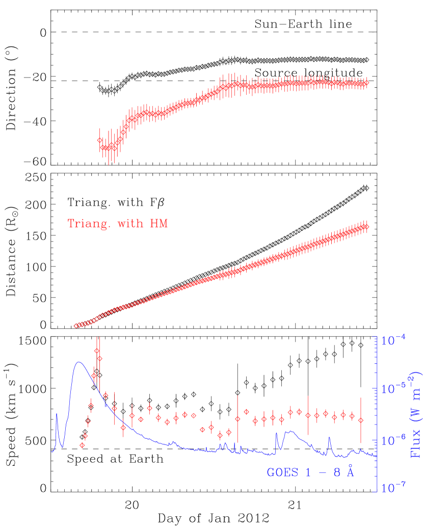
Figure 3: Propagation direction, radial distance and speed profiles of the leading edge of the 2012 January 19 CME derived from triangulation with F$\beta$ (black) and HM (red) approximations. The Sun-Earth line and the longitude of the CME source location on the Sun are indicated by the dashed lines in the top panel. The speeds are calculated from adjacent distances using a numerical differentiation with three-point Lagrangian interpolation, and then every three points after the acceleration phase are binned, so shown after the acceleration phase are average values and standard deviations within the bins. The dashed line in the bottom panel marks the average solar wind speed in the sheath region behind the shock observed in situ near the Earth. Overlaid on the speeds is the GOES X-ray flux (scaled by the blue axis).

Characterizing CME Sun-to-Earth propagation is a primary scientific question that STEREO was designed to address and the greater heliospheric constellation enables. Although studies have been performed attempting to connect STEREO heliospheric imaging observations with in situ signatures at 1 AU (e.g., Davis et al., 2009; Wood et al., 2009; Rouillard et al., 2009; Möstl et al., 2009, 2010; Liu et al., 2010a, b, 2011, 2012; Harrison et al., 2012; Temmer et al., 2012; Lugaz et al., 2012; Webb et al., 2013), there is much to learn on how to properly interpret these combined data sets and their information on CME propagation from the Sun to the Earth. A major limitation is the inherent difficulties involved in interpreting the heliospheric imaging observations. A popular approach is to fit CME tracks in time-elongation maps reconstructed from the wide-angle imaging observations by assuming a kinematic model (e.g., Sheeley et al., 2008; Rouillard et al., 2008; Lugaz, 2010a; Möstl et al., 2011; Davies et al., 2012). CMEs are assumed to travel along a constant direction at a constant speed in these models. A recent statistical analysis indicates that these track fitting techniques, while useful, give rise to a dependence between the free parameters (Davies et al., 2012, see their Figure 3). Clearly, the degeneracy between the free parameters cannot be broken in a fitting technique, so the solutions are not unique. Liu et al. (2010a, b) have developed a geometric triangulation technique using the stereoscopic imaging observations from STEREO. The uniqueness of this method is that it has no free parameters and can determine CME kinematics as a function of distance, which provides an unprecedented opportunity to probe CME propagation and interaction with the heliosphere. The technique has had success in tracking CMEs and connecting imaging observations with in situ signatures for various CMEs and spacecraft longitudinal separations (Liu et al., 2010a, b, 2011, 2012; Möstl et al., 2010; Harrison et al., 2012; Temmer et al., 2012). It assumes that the two spacecraft observe generally the same part of a CME, which, however, may not be always true, especially for extreme cases like the events studied here (very wide and back-sided for STEREO). Lugaz et al. (2010b) and Liu et al. (2010b) realize that the triangulation concept can be applied with a harmonic mean (HM) approach, which assumes that CMEs have a spherical front attached to the Sun and what is seen by a spacecraft is the segment tangent to the line of sight (Lugaz et al., 2009). The HM approximation is intended for wide CMEs only. Also note that CMEs can be significantly distorted by ambient coronal and solar wind structures (e.g., Riley & Crooker, 2004; Liu et al., 2006, 2008b, 2009b). It would be interesting to compare results from the two triangulation techniques, which is one of the purposes of this paper. It should be kept in mind that the present CMEs are extreme cases, i.e., very wide and back-sided events for STEREO. Any discussions and implications on the advantages and disadvantages of the two triangulation methods based on the results should be taken with caution.

This paper has a threefold aim: (1) to constrain CME Sun-to-Earth propagation using coordinated heliospheric imaging, radio and in situ observations; (2) to compare different techniques with which to determine CME kinematics in interplanetary space; (3) to investigate crucial physical processes governing CME propagation and interaction with the heliosphere. This work requires heliospheric imaging observations from both STEREO A and B, interplanetary radio type II bursts of a sufficiently long duration (so that comparison with wide-angle heliospheric imaging observations is meaningful), and in situ signatures at 1 AU. Due to the last long solar minimum, long-duration interplanetary type II bursts have only been available since 2011 (http://lep694.gsfc.nasa.gov/waves/data_products.html). By this time, the two STEREO spacecraft were already behind the Sun, so the Earth-directed CMEs after 2011 (February) are essentially back-sided events for STEREO. From their vantage points behind the Sun, the two spacecraft are likely observing different parts of an Earth-directed CME when it is at large distances. In particular, CMEs that are associated with a long-duration interplanetary type II burst are usually wide events. This is why triangulation with the HM approximation is likely to be necessary. Observations and methodology are described in Section 2. We present details on case studies in Section 3. The results are summarized and discussed in Section 4. To the best of our knowledge, this is the first study that attempts to create a general picture of CME Sun-to-Earth propagation combining wide-angle heliospheric imaging observations, interplanetary type II bursts and in situ measurements at 1 AU. Our findings on CME Sun-to-Earth propagation provide a test bed or benchmark for CME Sun-to-Earth research and space weather prediction. New insights obtained from this work will improve observational strategies and analysis tools. Specifically, this work evaluates a triangulation concept for future CME observations and space weather forecasting, a key strategic study to prepare for future missions at L4/L5.

2 Observations and Methodology

We pick three events for this study, i.e., the 2012 January 19, 23 and March 7 CMEs. Each of these events has wide-angle imaging coverage from both STEREO A and B, a long-duration interplanetary type II burst, and in situ signatures near the Earth. These are extreme cases, i.e., wide and back-sided for STEREO. Below we describe the observations and methodology used for the joint interpretation of the different data sets.

2.1 Geometric Triangulation of Imaging Observations

Of particular interest for this study are the heliospheric imagers (HI1 and HI2) on board STEREO. They can observe CMEs out to the vicinity of the Earth and beyond by using sufficient baffling to eliminate stray light (Harrison et al., 2008; Eyles et al., 2009). The combined effects of projection, Thomson scattering and CME geometry, however, form a major challenge in determining CME kinematics from the wide-angle imaging observations. The geometric triangulation technique developed by Liu et al. (2010a, b) can determine both propagation direction and radial distance of CMEs from STEREO imaging observations, assuming a fixed $\beta$ (F$\beta$) geometry, i.e., a relatively compact structure simultaneously seen by the two spacecraft. (The F$\beta$ approximation was initially used for track fitting, which assumes a compact structure moving along a fixed radial direction (Sheeley et al., 1999; Kahler & Webb, 2007; Liu et al., 2010b). This is where the term “fixed” comes from. When the F$\beta$ formula is adopted for geometric triangulation, the assumption of fixed radial trajectory is abolished.) Hereinafter we call the technique triangulation with the F$\beta$ approximation. Liu et al. (2010a, b) describe the mathematical formulas and detailed procedures for applying this technique. The F$\beta$ triangulation gives good results in analysis of Earth-oriented CMEs when the two spacecraft are before the Sun (Liu et al., 2010a, b, 2011, 2012; Möstl et al., 2010; Harrison et al., 2012; Temmer et al., 2012). Now we evaluate its use on those wide and back-sided events.

We also apply the triangulation concept under a harmonic mean (HM) approximation, which takes into account the effect of CME geometry. It assumes that a CME has a spherical front attached to the Sun, and the two spacecraft observe different plasma parcels that lie along the tangent to their line of sight (Lugaz et al., 2009). Hereinafter we refer to it as triangulation with the HM approximation. Both of the triangulation techniques have no free parameters, and can determine CME kinematics as a function of distance from the Sun continuously out to 1 AU. These advantages make the techniques a powerful tool for investigating CME Sun-to-Earth propagation and forecasting space weather. The readers are directed to Liu et al. (2010b) and Lugaz et al. (2010b) for more detailed discussions of these two triangulation techniques. In this work, we apply the two methods to the imaging observations of COR2, HI1 and HI2. COR1 images are also examined but not included here given its small FOV. Therefore, the resulting CME kinematics do not include the initiation phase of CMEs. We will compare the two methods using the current cases and see how they work as we move from small to large distances. We will also investigate how their results compare with other data sets.

2.2 Frequency Drift of Radio Type II Bursts

Interplanetary radio type II bursts associated with CMEs provide further constraints on CME Sun-to-Earth propagation. Type II bursts, typically drifting downward in frequency, are plasma radiation near the local plasma frequency and/or its second harmonic produced by a shock (e.g., Nelson & Melrose, 1985; Cane et al., 1987). The frequency drift results from the decrease of the plasma density as the shock moves away from the Sun, so the shock propagation distance can be inverted from the type II burst by assuming a density model (e.g., Reiner et al., 2007; Liu et al., 2008a; Gonzalez-Esparza & Aguilar-Rodriguez, 2009). In this study, we use a density model which covers a distance range from about 1.8 solar radii to 1 AU (Leblanc et al., 1998, hereinafter referred to as the Leblanc density model). The Leblanc density model is scaled by a density of 6.5 cm^-3 at 1 AU, the average value of Wind measurements over a few months around the CME times. The same density model is applied to all the three events.

Note that the density model describes an average radial variation of the ambient solar wind density, so we do not expect that it fits the band of a type II burst all the times. Recent work has shown that the source position of a type II burst at a particular frequency can be triangulated without using a density model (Martinez-Oliveros et al., 2012), but that technique requires a strong radio emission seen by more than one spacecraft. The current cases are all back-sided events for STEREO, and strong type II bursts are only observed by Wind. This work is intended to compare wide-angle heliospheric imaging observations with long-duration interplanetary type II bursts. In doing this we explicitly assume that the distances inverted from a type II burst, which essentially represent shock kinematics, do not deviate much from the distances of the leading edge seen in white light. The geometric triangulation described above is applied to the leading feature in imaging observations, which could be a high-density structure in the sheath between the shock and ejecta or the shock itself as revealed by previous studies (Liu et al., 2011, 2012).

2.3 Comparison with In Situ Measurements

The CME kinematics inferred from imaging observations and type II bursts will be compared with in situ measurements at Wind, another step in our analysis. CMEs are called interplanetary CMEs (ICMEs) when they move into the solar wind. In situ measurements can give local plasma and magnetic field properties along a one-dimensional cut when ICMEs encounter spacecraft. Signatures used to identify ICMEs from solar wind measurements include depressed proton temperatures, enhanced helium/proton density ratio, smooth magnetic fields, and rotation of the field. In this paper we use the term “CMEs” for events observed in images and “ICMEs” for ejecta identified from in situ measurements. Our comparison with in situ data mainly focuses on CME speed and arrival time at the Earth. The connections between imaging observations, type II bursts and in situ signatures can also indicate the nature of structures observed in images, e.g., shocks and flux ropes (Liu et al., 2010a, b, 2011, 2012; DeForest et al., 2011).

3 Case Studies

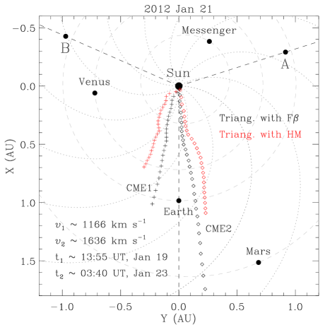
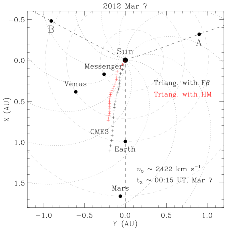
Figure 1: Positions of the spacecraft and planets in the ecliptic plane on 2012 January 21 (left) and 2012 March 7 (right). The gray dashed curves indicate the planetary orbits, and the dotted lines show Parker spiral magnetic fields created with a solar wind speed of 450 km s^-1. The trajectories of the CMEs of interest, which are obtained from triangulation with the F$\beta$ approximation (black) and triangulation with the HM approximation (red), respectively, are marked by crosses for CME1 and CME3 and diamonds for CME2. The estimated CME peak speed and launch time on the Sun are also given. Note that the two STEREO spacecraft were observing the CMEs from behind the Sun.

Figure 1 shows the trajectories of the CMEs of interest as well as the configuration of the planets and spacecraft in the ecliptic plane. STEREO A and B are separated by about 221.1^∘ in longitude (the angle bracketing the Earth) on 2012 January 19, about 221.7^∘ on January 23 and about 227.1^∘ on March 7, respectively. Triangulation with the HM approximation gives a propagation angle with respect to the Sun-Earth line roughly twice of that from triangulation with the F$\beta$ approximation, as previously indicated by Lugaz (2010a). During the 2012 March 7 CME, Mars was at 1.66 AU from the Sun and almost radially aligned with the Earth, so the March 7 CME was likely to impact both the Earth and Mars. Enhanced fluxes of energetic particles were indeed observed by Curiosity, when it was traveling to Mars inside the Mars Science Laboratory spacecraft (http://science.nasa.gov/science-news/science-at-nasa/2012/02aug_rad2/).

3.1 2012 January 19 Event

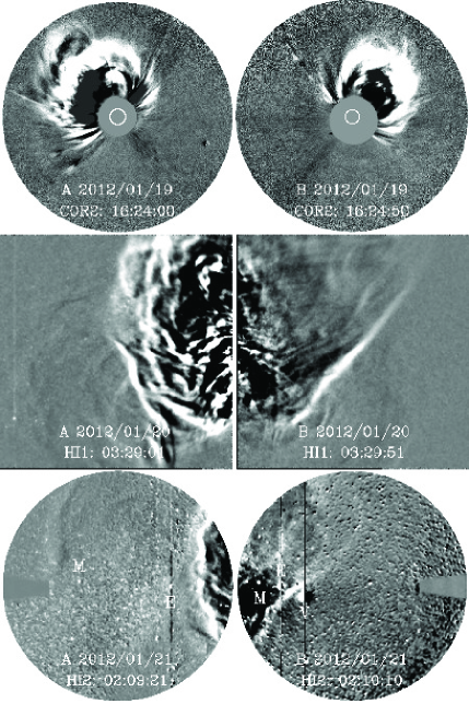
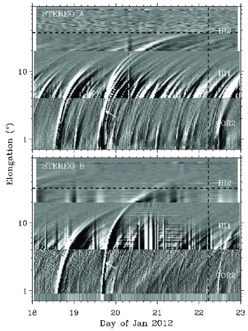
Figure 2: Left: Evolution of the 2012 January 19 CME observed by STEREO A and B near simultaneously. From top to bottom, the panels show the running difference images from COR2, HI1 and HI2, respectively. The positions of the Earth (E), Mars (M) and Venus (V) are labeled in the HI2 images. Note a preceding CME visible to COR2 of STEREO A. Right: Time-elongation maps constructed from running difference images of COR2, HI1 and HI2 along the ecliptic plane for STEREO A (upper) and B (lower). The arrow indicates the track associated with the CME of interest. The vertical dashed line shows the observed arrival time of the CME-driven shock at the Earth, and the horizontal dashed line marks the elongation angle of the Earth.

The 2012 January 19 CME originated from NOAA AR 11402 (N32^∘E22^∘), and is associated with a long-duration M3.2 flare which peaked around 16:05 UT on January 19. Figure 2 (left) displays two synoptic views of the CME from STEREO A and B. Only shown are images from COR2, HI1 and HI2. COR2 has a 0.7^∘ - 4^∘ FOV around the Sun. HI1 has a 20^∘ square FOV centered at 14^∘ elongation from the center of the Sun while HI2 has a 70^∘ FOV centered at 53.7^∘. The CME is launched from the Sun at about 13:55 UT on January 19 and has a peak speed of about 1200 km s^-1 (see Figure 1). Deflections of remote coronal structures are observed in COR2 images, which suggest the existence of the CME-driven shock (e.g., Vourlidas et al., 2003; Liu et al., 2009a). The CME looks quite different for STEREO A and B, especially in HI1 and HI2, which may indicate the significant effect on the CME of the medium through which it is propagating. Figure 2 (right) shows the time-elongation maps, which are produced by stacking the running difference intensities of COR2, HI1 and HI2 within a slit around the ecliptic plane (e.g., Sheeley et al., 2008; Davies et al., 2009; Liu et al., 2010a). Multiple tracks are observed on January 18 - 19, so CME-CME interactions are likely present. In particular, a CME from January 18 and another one that occurred a few hours earlier on January 19 are visible to both STEREO A and B, and could have effect on the interplanetary propagation of the CME of interest. In STEREO B observations the CME reaches the elongation of the Earth earlier than in STEREO A images, so it must propagate east of the Sun-Earth line.

We apply the two triangulation techniques to the leading feature of the CME in imaging observations, and the resulting CME kinematics in the ecliptic plane are displayed in Figure 3. Both of the methods give negative propagation angles (east of the Sun-Earth line), consistent with the solar source location and the time-elongation maps. The propagation angle from triangulation with the F$\beta$ approximation starts from about the solar source longitude, while the angle from triangulation with the HM approximation keeps about twice of the former and finally approaches the solar source longitude. Their trends are similar except that the HM approximation enlarges the variations. The distances from the two methods show no essential differences below about 70 solar radii, but after about 100 radii the F$\beta$ approximation gives an apparent acceleration. This late acceleration is also noticed in previous studies (e.g., Lugaz et al., 2009; Wood et al., 2009; Harrison et al., 2012). It is not physically meaningful, as there is no obvious force responsible for the acceleration at large distances from the Sun. A similar scenario is observed in the 2012 January 23 and March 7 CMEs. In the current cases the late acceleration at large distances is due to the non-optimal observation situation (from behind the Sun) in combination with the restrictions of the F$\beta$ geometry (see section 4.2).

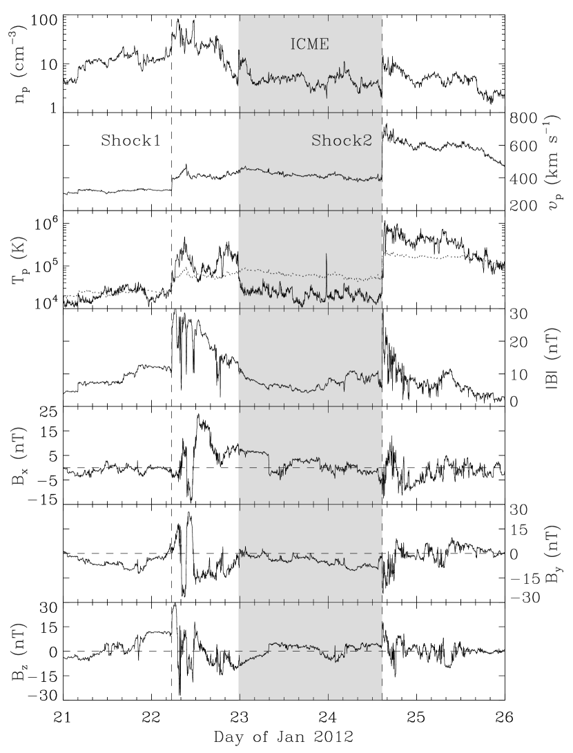
Figure 6: Solar wind plasma and magnetic field parameters across the ICME observed at Wind. From top to bottom, the panels show the proton density, bulk speed, proton temperature, and magnetic field strength and components, respectively. The dotted line in the third panel denotes the expected proton temperature from the observed speed. The shaded region indicates the ICME interval. The vertical dashed lines mark two shocks, the first one driven by the present ICME (in situ counterpart of the 2012 January 19 CME) and the second one by the 2012 January 23 CME. Note that the second shock is beginning to overtake the ICME from behind. The 2012 January 23 CME does not have in situ signatures at Wind (except the shock).

The speed profiles from the two triangulation methods are similar below about 60 solar radii, except that the peak speed from the HM approximation is a little higher. Both the speed profiles show an impulsive acceleration up to about 15 solar radii, then a rapid deceleration out to about 35 solar radii, and then a roughly constant value thereafter. The late increase in the speed profile from the F$\beta$ approximation, again, is considered unmeaningful. The CME is still accelerating even after the flare maximum, as indicated by the timing with the GOES X-ray curve. The CME speed peaks about 2.5 hours after the flare maximum, so energy must be continuously fed into the CME even after the time of the maximum heating and radiation has elapsed in the corona. The rapid deceleration, presumably due to interactions with the ambient medium, only lasts about 4 hours, a relatively short time scale. Therefore the maximum drag by, or energy loss to, the ambient medium takes place at distances not far from the Sun (within 35 solar radii). Similar results have been alluded to in other cases (e.g., Liu et al., 2010a, b, 2011). The HM approximation can suppress the late acceleration, but compared with the average solar wind speed behind the shock observed in situ near the Earth, it still overestimates the speed by about 250 km s^-1 (see Figure 6).

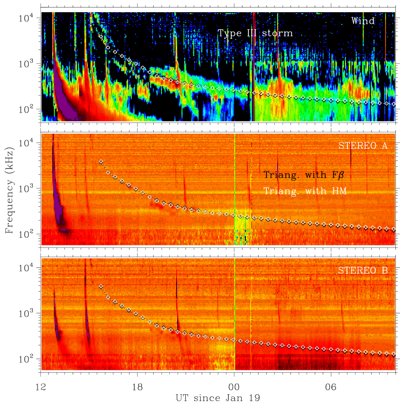
Figure 4: Dynamic spectrum (color shading) associated with the 2012 January 19 CME from Wind, STEREO A and B. The CME leading edge distances derived from triangulation with F$\beta$ (black) and HM (white) approximations are converted to frequencies by using the Leblanc density model, which are then plotted over the dynamic spectrum. Note a type III storm observed by Wind, which seems to have an overall drift rate similar to that of the type II burst.

Figure 4 shows the radio dynamic spectrum associated with the CME. Strong type II emissions are only observed by Wind. They occur at the fundamental and harmonic plasma frequencies and appear as slowly drifting features. The type II burst starts from the upper bound (16 MHz) around 15:00 UT on January 19 and extends down to about 150 kHz. We use an approach different from previous studies: the CME leading-edge distances derived from imaging observations are converted to frequencies using the Leblanc density model (with a density of 6.5 cm^-3 at 1 AU), given that we already have the distances. The imaging triangulation results are generally consistent with the type II burst, and there is no essential difference between the F$\beta$ and HM approximations for the time period covered by the figure. The weak type II emissions observed by STEREO A and B, e.g., those at 400 kHz around 19:30 UT on January 19, are also captured by the triangulation results. The consistency between the imaging results and radio data from three spacecraft suggests the validity of our triangulation concept. It may also indicate a relationship between the CME leading feature being tracked and the type II burst, but a careful study is needed to reach a definite conclusion. Note that many short-lived type III like bursts, known as a type III storm (e.g., Fainberg & Stone, 1970), are also observed by Wind. This type III storm seems to have an overall drift rate similar to that of the type II burst, which may hold an important clue about the origin of the type III storm.

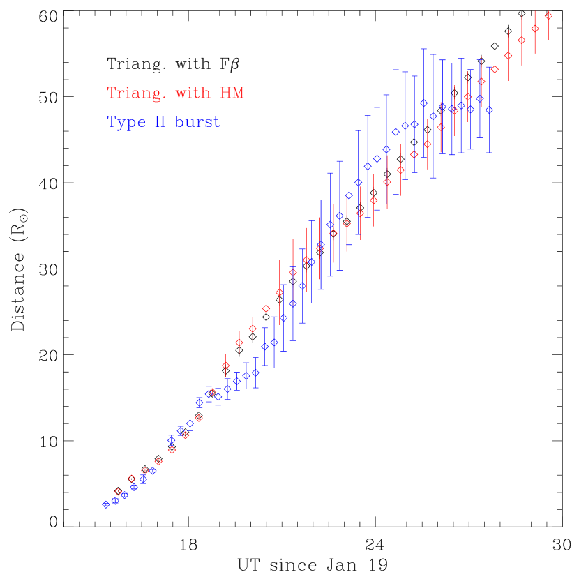
Figure 5: Comparison between the CME leading edge distances derived from triangulation with F$\beta$ (black), triangulation with HM (red), and the radio type II burst (blue).

The frequencies of the type II burst (assuming the harmonic branch) are also converted to distances using the Leblanc density model, as shown in Figure 5. The error bars in the radio data are determined from the band width of the type II burst. Again, we see a general consistency between the imaging triangulation results and the type II burst, and there is no essential difference between the F$\beta$ and HM approximations below 60 solar radii. There appears to be a decrease in the drift rate of the type II burst after about 02:00 UT on January 20, while the CME does not seem to have an apparent slowdown at the same time.

Figure 6 shows an ICME identified from Wind in situ measurements based on the depressed proton temperature and smooth magnetic field. The ICME interval is also consistent with the decreased proton beta. This is the in situ counterpart of the 2012 January 19 CME. The CME-driven shock (shock1) passed Wind at about 05:28 UT on January 22. The average speed in the sheath region between the shock and ICME is about 415 km s^-1, which is about 250 km s^-1 lower than predicted by triangulation with the HM approximation (see Figure 3). The predicted arrival time at the Earth is about 08:10 UT on January 21 resulting from triangulation with the F$\beta$ approximation and 03:11 UT on January 22 given by the HM triangulation. We have used $r\cos\beta$ and $v\cos\beta$ for the HM approach in estimating the arrival time and speed at the Earth, respectively, where $r$ is the distance from imaging observations, $v$ the speed, and $\beta$ the propagation angle with respect to the Sun-Earth line. The much earlier prediction from the F$\beta$ triangulation compared with the observed shock arrival is probably owing to the unphysical late acceleration at large distances. The HM triangulation does a very good job in predicting the shock arrival, although it overestimates the speed considerably. Compared with the speed near the Sun ($\sim 1200$ km s^-1), the ICME/shock is significantly decelerated by the structured solar wind. The second shock (shock2), which is also the trailing boundary of the ICME, is driven by the 2012 January 23 CME. The shock passed Wind at about 14:38 UT on January 24, and is beginning to overtake the ICME from behind.

3.2 2012 January 23 Event

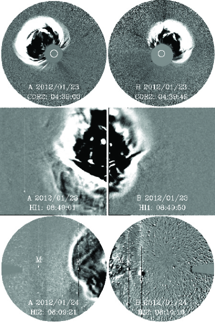
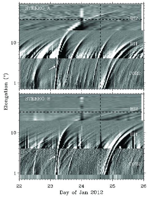
Figure 7: Similar to Figure 2, but for the 2012 January 23 CME. Note a transition layer around the CME front in COR2, reminiscent of a shock signature.

The 2012 January 23 CME originated from NOAA AR 11402 (N29^∘W20^∘), the same active region as the 2012 January 19 event, and is associated with a long-duration M8.7 flare which peaked around 03:59 UT on January 23. Figure 7 (left) displays two views of the CME from STEREO A and B. The CME is launched from the Sun at about 03:40 UT on January 23 and has a peak speed of about 1600 km s^-1 (see Figure 1). A weak edge ahead of the CME front is visible in COR2, reminiscent of a shock signature (e.g., Vourlidas et al., 2003; Liu et al., 2008a). Only part of the CME is seen in HI1 and HI2, indicating the need for a bigger FOV in future CME heliospheric imaging observations. In HI2 of STEREO A, the CME leading feature (which could be the shock) appears as a grand wave sweeping over the inner heliosphere, while the driver can hardly be seen. This must be part of the evolutionary history of the densities in the ejecta and sheath (Liu et al., 2011). Figure 7 (right) shows the time-elongation maps produced from intensities around the ecliptic. Again, other tracks are observed around the time of the CME, so CME-CME interactions are expected. The CME must propagate west of the Sun-Earth line, since in STEREO A observations it reaches the Earth’s elongation earlier than in STEREO B.

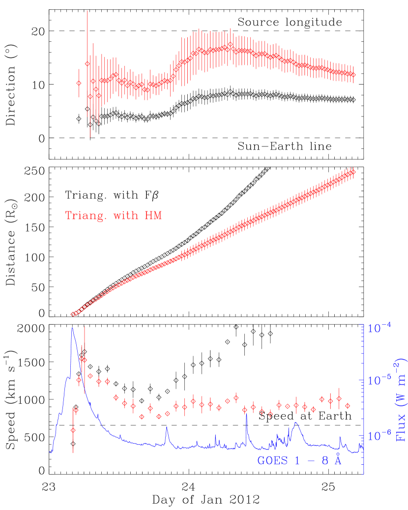
Figure 8: Similar to Figure 3, but for the 2012 January 23 CME.

The CME kinematics resulting from the two triangulation techniques are shown in Figure 8. The two methods give positive propagation angles (west of the Sun-Earth line), consistent with the solar source location and the time-elongation maps. However, the propagation angles from both of the techniques deviate from the solar source longitude, which may suggest longitudinal deflections of the CME at its early stage. Again, the trends in the angles are similar for the F$\beta$ and HM approximations, and the angle from the HM approach keeps about twice of that from the F$\beta$ approximation. The F$\beta$ approach gives an unphysical acceleration after about 100 solar radii, which is due to the non-optimal observation situation (from behind the Sun) and the F$\beta$ geometry as discussed above. The speed profiles from the two triangulation methods are similar below about 75 solar radii. Both the speed profiles show an impulsive acceleration up to about 16 solar radii, and then a rapid deceleration out to about 75 solar radii. The CME is still accelerating even after the flare maximum. The maximum speed lags the peak of the GOES X-ray curve by about 2 hours. The rapid deceleration lasts about 10 hours in this case. The HM approximation overestimates the observed solar wind speed at the Earth by about 250 km s^-1 (see Figure 6), although it suppresses the late acceleration.

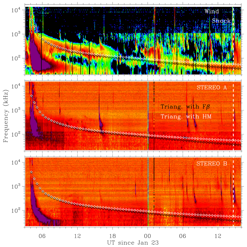
Figure 9: Similar to Figure 4, but for the 2012 January 23 event. The vertical dashed line indicates the observed arrival time of the CME-driven shock at the Earth.

Figure 9 displays the radio dynamic spectrum associated with the 2012 January 23 CME. Strong type II emissions are only observed by Wind. The type II burst starts from the upper bound (16 MHz) around 04:10 UT on January 23, and extends down to about 40 kHz when the shock arrives at Wind (14:38 UT on January 24). Apparently this is a Sun-to-Earth type II burst. Weak type II spots are observed by STEREO A (e.g., those near 200 kHz around 13:00 UT on January 23 and near 70 kHz around 06:30 UT on January 24), but not STEREO B. This indicates that the propagation direction is closer to STEREO A than B, consistent with the triangulation results. The CME leading-edge distances from imaging observations, after being converted to frequencies using the Leblanc density model (with a density of 6.5 cm^-3 at 1 AU), are generally consistent with the type II burst. Here we assume that the strong type II band observed by Wind is emitted at the second harmonic of the local plasma frequency. The weak type II emissions observed by STEREO A are also captured by the triangulation results, again indicating the validity of our triangulation concept. At large distances the F$\beta$ approach appears to fit the type II burst better than HM, which is not what we expect.

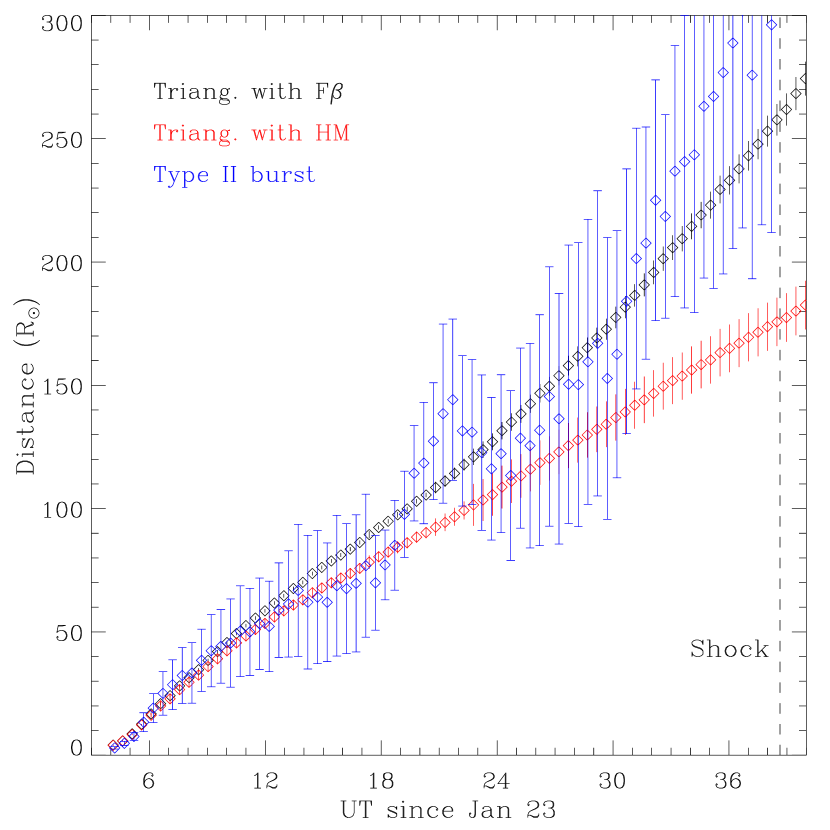
Figure 10: Similar to Figure 5, but for the 2012 January 23 CME. The vertical dashed line indicates the observed arrival time of the CME-driven shock at the Earth.

Figure 10 shows the distances derived from the type II burst using the Leblanc density model, in a comparison with triangulation analysis. There is essentially no difference between the F$\beta$ and HM approximations below about 70 solar radii. The F$\beta$ approximation is more consistent with the type II burst than HM at large distances, as we see from Figure 9. It is not clear about the cause of the late increase in the frequency drift of the type II burst. Perhaps the shock is propagating into a less dense medium at large distances, or it is due to complexities in the radio emission region. The shock driven by the 2012 January 23 CME (shock2) passed Wind at about 14:38 UT on January 24, as shown in Figure 6, and is propagating into the ICME associated with the January 19 event. The ICME preceding the shock does have a depressed proton density at 1 AU compared with the ambient medium. The average speed behind the shock is about 650 km s^-1, again about 250 km s^-1 lower than predicted by the HM triangulation. Triangulation with the F$\beta$ approximation gives a predicted arrival time at the Earth of about 09:42 UT on January 24, while the HM triangulation yields a predicted arrival time of about 23:06 UT on January 24. Again, we have used $r\cos\beta$ and $v\cos\beta$ in estimating the arrival time and speed at the Earth for the HM approach. It is surprising that the F$\beta$ triangulation does a better job than the HM approach in predicting the shock arrival. A possible explanation is that the shock was propagating through the preceding ICME at large distances, which is less dense than the ambient solar wind. This might compensate for the the unphysical late acceleration given by the F$\beta$ triangulation. The 2012 January 23 CME does not have in situ signatures at Wind (except the shock). It is likely that the CME missed Wind, and the shock must have a structure larger than the ejecta or flux rope.

3.3 2012 March 7 Event

March 2012 is a very interesting period, during which a series of M/X class flares and big CMEs occurred. In particular, NOAA AR 11429 generated an X1.1 flare and a CME of about 1500 km s^-1 around 03:00 UT on March 5, an X5.4 flare and a CME of more than 2000 km s^-1 around 00:15 UT on March 7, an M6.3 flare and a CME of about 1000 km s^-1 around 03:30 UT on March 9, an M8.4 flare and a CME of more than 1000 km s^-1 around 17:30 UT on March 10, and an M7.9 flare and a CME of over 1500 km s^-1 around 17:30 UT on March 13. Among them the March 7 CME is the largest and most energetic. There seems another event on March 7, which occurred about 1 hour later than the first one. It produced an X1.3 flare and a CME of over 1500 km s^-1. The second CME is occulted by the first one in STEREO coronagraph images, as it occurred close in time with the first one. At least three of the events hit the Earth, including the March 5, 7 and 10 events (see Figure 15).

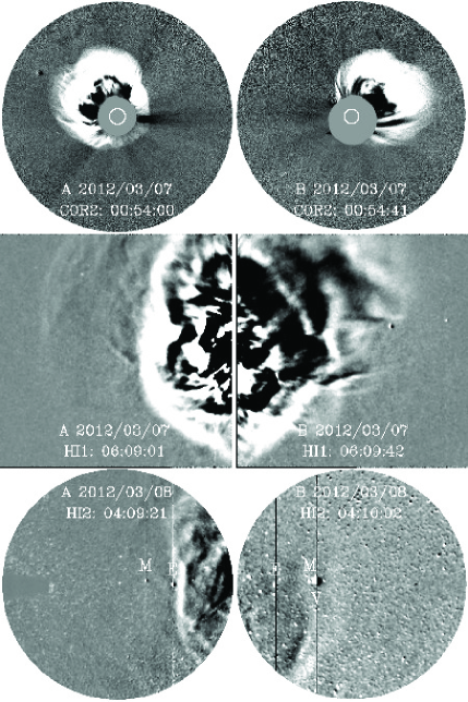
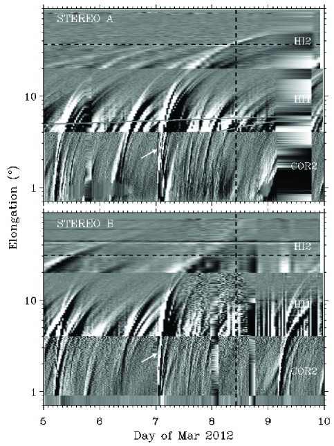
Figure 11: Similar to Figure 2, but for the 2012 March 7 CME. A weak edge around the CME front is also observed in COR2.

The violent corona and heliosphere during the March 7 CME are shown in Figure 11 (left), as seen from STEREO A and B. NOAA AR 11429 was at N17^∘E21^∘ when the CME occurred, and the associated long-duration X5.4 flare peaked around 00:24 UT on March 7. The CME is launched from the Sun at about 00:15 UT and has a peak speed of about 2400 km s^-1 (see Figure 1). A weak edge around the CME front is observed in COR2, indicative of a shock signature (e.g., Vourlidas et al., 2003; Liu et al., 2008a). The heliosphere observed by HI1 and HI2 is very turbulent when the series of dramatic CMEs blow through their FOVs. Figure 11 (right) shows the time-elongation maps produced from intensities around the ecliptic. We observe multiple tracks from the maps, some of which cross, which suggests CME-CME interactions. The CME must propagate east of the Sun-Earth line, since in STEREO B observations it reaches the Earth’s elongation earlier than in STEREO A.

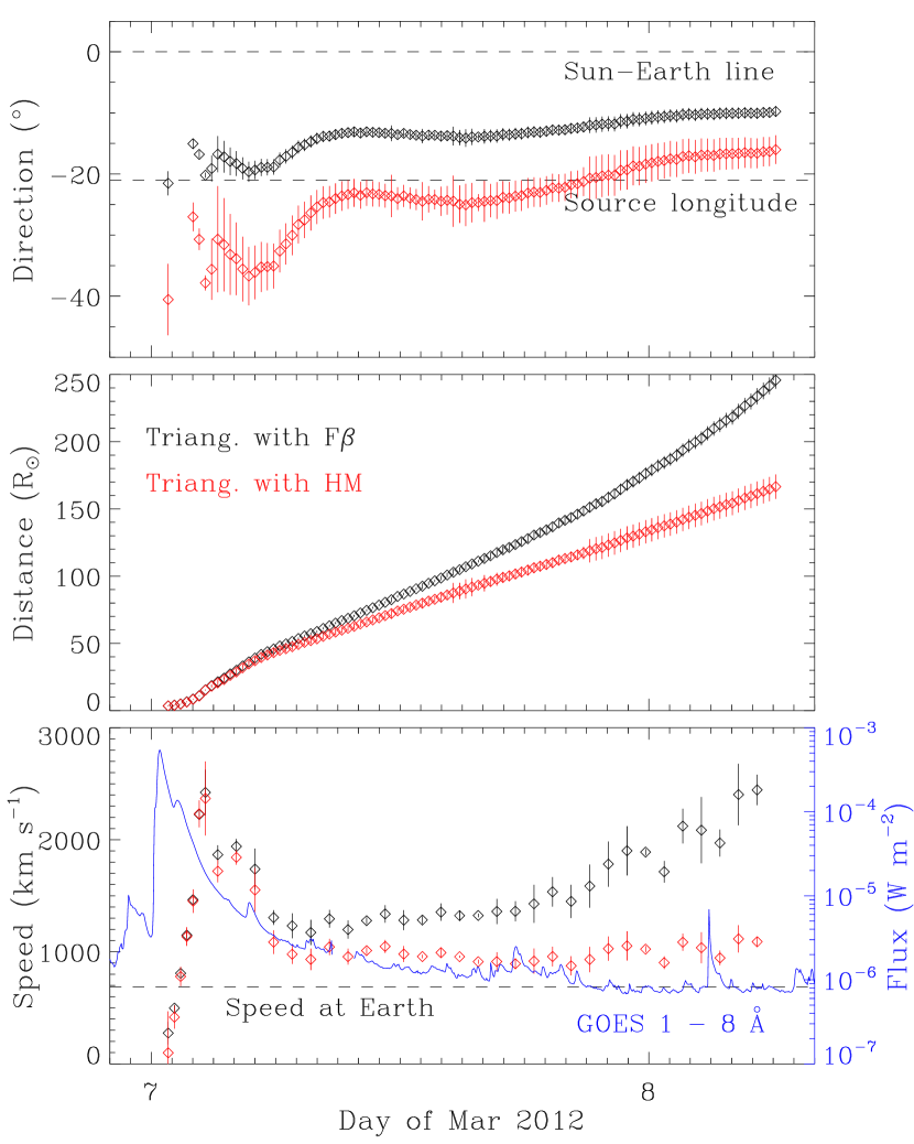
Figure 12: Similar to Figure 3, but for the 2012 March 7 CME.

The kinematics of the CME leading feature resulting from the two triangulation techniques are shown in Figure 12. Both of the methods give negative propagation angles (east of the Sun-Earth line), consistent with the solar source location and the time-elongation maps. Similar to the January 19 event, the propagation angle from triangulation with the F$\beta$ approximation starts from about the solar source longitude. The angle from triangulation with the HM approximation still keeps about twice of that from the F$\beta$ approximation. The F$\beta$ approach gives an unphysical acceleration after about 120 solar radii, which is due to the non-optimal observation situation (from behind the Sun) and the assumed CME geometry. There is also a slight acceleration in the HM approach at large distances, which suggests that the HM approximation is not adequate to suppress the apparent late acceleration in this case. The speed profiles from the two triangulation methods are similar below about 70 solar radii. Both the speed profiles show an impulsive acceleration up to about 15 solar radii, then a rapid deceleration out to about 55 solar radii, and then a roughly constant value thereafter. The CME is still accelerating even after the flare maximum. The maximum speed occurs about 2 hours after the peak of the GOES X-ray curve. The rapid deceleration lasts about 5 hours in this case. The HM approximation overestimates the observed solar wind speed at the Earth by about 270 km s^-1 (see Figure 15).

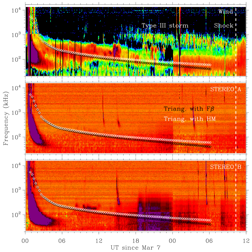
Figure 13: Similar to Figure 4, but for the 2012 March 7 event. The vertical dashed line indicates the observed arrival time of the CME-driven shock at the Earth.

Figure 13 displays the radio dynamic spectrum associated with the 2012 March 7 CME. Strong type II emissions are only observed by Wind. The type II burst starts from the upper bound (16 MHz) around 01:15 UT on March 7, and extends down to about 40 kHz by the time the shock arrives at Wind (10:19 UT on March 8). This is a Sun-to-Earth type II burst and probably the strongest one in solar cycle 24 up to the time of this writing. Weak type II spots are observed by STEREO B, e.g., those near 200 kHz around 10:00 UT on March 7, while below 1000 kHz no type II emissions are observed by STEREO A. This indicates that the propagation direction is closer to STEREO B than A, consistent with the triangulation results. The CME leading-edge distances from imaging observations, after being converted to frequencies using the Leblanc density model (with a density of 6.5 cm^-3 at 1 AU), are generally consistent with the type II burst. We assume that the type II band we are comparing is emitted at the second harmonic of the local plasma frequency. The imaging triangulation results also capture the weak type II emissions observed by STEREO A and B, which again indicates the validity of our triangulation concept. At large distances the HM approach fits the type II burst better than F$\beta$. A type III storm, whose overall drift rate is similar to that of the type II burst, is also observed by Wind (above the type II burst).

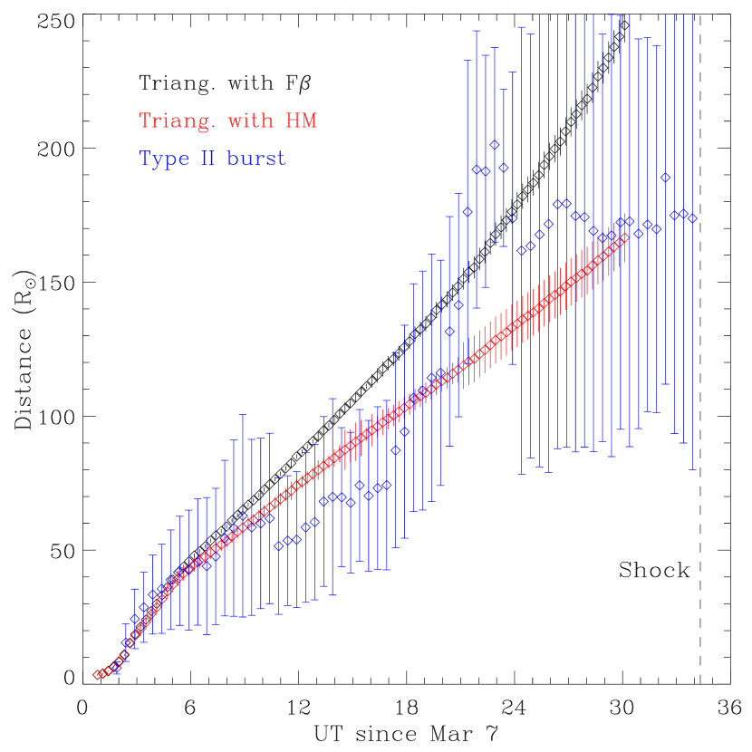
Figure 14: Similar to Figure 5, but for the 2012 March 7 CME. The vertical dashed line indicates the observed arrival time of the CME-driven shock at the Earth.

Figure 14 shows the comparison between the distances derived from the type II burst using the Leblanc density model and triangulation analysis. There is no essential difference between the F$\beta$ and HM approximations below about 50 solar radii. The HM approximation is more consistent with the type II burst than F$\beta$ after March 7, as we see from Figure 13. The type II burst suggests a quick deceleration on March 8, but the large error bars (from the band width of the type II burst) do not allow determination of how much the shock is slowed down. Irregularities in the type II burst, which come from the non-uniformity of the ambient density, may contribute to the apparent deceleration.

The in situ signatures at Wind are shown in Figure 15. Two ICMEs are identified during the time period using the depressed proton temperature and smooth magnetic field. The first one (ICME1) and its shock (S1) are produced by the March 7 CME, and the second (ICME2) and its shock (S2) by the March 10 event. A weak shock (S0) preceding S1 seems driven by a CME from March 5, but no driver signatures are observed (except the shock). Interactions between the March 5 and 7 CMEs are likely to have occurred near 1 AU. The ICMEs, shocks and possible interactions between them caused a long duration (from March 7 to March 19) of significant negative values of the D_st index. In particular, ICME1 (and S1) produced a major geomagnetic storm with a minimum D_st of $-143$ nT. The shock driven by the March 7 CME (S1) passed Wind at about 10:19 UT on March 8. The average speed in the sheath behind S1 is about 680 km s^-1, about 270 km s^-1 lower than predicted by the HM approximation. Triangulations with the F$\beta$ and HM approximations give a predicted arrival time at the Earth of about 03:27 UT and 17:55 UT on March 8, respectively. Compared with the actual shock arrival time (10:19 UT), these predictions appear equally good, but the F$\beta$ prediction is earlier than the observed shock arrival and the HM one lies in the sheath. This raises a question in space weather studies (and forecasting as well): what in situ signatures should we compare with, the shock or the leading edge of the flux rope? Previous studies attempting to connect imaging observations with in situ measurements indicate that what is being tracked is often a high-density structure in the sheath or the shock itself (Liu et al., 2011, 2012). The ICME/shock is again significantly decelerated by the structured solar wind, compared with the speed near the Sun ($\sim 2400$ km s^-1).

4 Conclusions and Discussion

To the best of our knowledge, this is the first comprehensive study that attempts to generalize the whole Sun-to-Earth propagation of CMEs combining heliospheric imaging observations, interplanetary radio type II bursts and in situ measurements from multiple vantage points. We summarize and discuss our results as follows, based on the case studies of the 2012 January 19, 23 and March 7 CMEs.

4.1 Formulating CME Sun-to-Earth Propagation

Key findings are revealed on how CMEs propagate through, and interact with, the entire inner heliosphere between the Sun and Earth. Below we formulate CME Sun-to-Earth propagation. Any theory/model of CME Sun-to-Earth propagation and space weather forecasting should be guided and constrained by the results presented here.

1. The Sun-to-Earth propagation of fast CMEs can be approximately described by three phases: an impulsive acceleration, then a rapid deceleration, and finally a nearly constant speed propagation (or gradual deceleration). The initiation phase in the low corona is not included in this study. We alluded to similar results in our triangulation analysis of the 2008 December 12 CME (Liu et al., 2010a, b) and the 2010 April 3 CME (Liu et al., 2011). It should be stressed that we are looking at CME propagation in the whole Sun-Earth space, not just within 20-30 solar radii as in some previous studies (e.g., Sheeley et al., 1999; Zhang et al., 2001). The speed of fast CMEs during the gradual deceleration phase is expected to approach that of the ambient solar wind. This should be a long process (out to several tens of AU from the Sun) as the energy is slowly dissipated into the ambient medium (e.g., Richardson et al., 2005; Liu et al., 2008a). The three phases hold only for fast events. CMEs slower than the ambient solar wind are expected to be accelerated by the solar wind (e.g., Sheeley et al., 1999, and references therein).

2. The CMEs studied here are still accelerating even after the flare maximum, so energy must be continuously fed into the CME even after the time of the maximum heating and radiation has elapsed in the corona. Zhang et al. (2001) suggest that CME acceleration occurs simultaneously with the flare impulsive phase and ceases near the peak of the GOES X-ray curve. Here we find further acceleration post the flare maximum with a time scale of about 2 hours. This is not uncommon (e.g., Cheng et al., 2010; Zhao et al., 2010; Liu et al., 2011). A statistical analysis indicates that the post-flare-maximum acceleration tends to occur in cases associated with a long-duration flare (Cheng et al., 2010). The time scale of CME further acceleration after the flare maximum may depend on the balance between energy injection from the Sun and drag by the ambient medium.

3. The rapid deceleration, presumably due to interactions with the ambient medium, mainly occurs over a relatively short time scale following the acceleration phase. The maximum drag by, or energy loss to, the ambient medium takes place at distances not far from the Sun. The rapid deceleration lasts about 5-10 hours and stops around 40-80 solar radii from the Sun for the current cases. The short cessation distance of CME deceleration is a surprising finding compared with previous indirect inferences (Gopalswamy et al., 2001a; Reiner et al., 2007). While drag by the ambient medium may play an important role in decelerating CMEs, we expect that a significant portion of the energy goes into energetic particles through shock acceleration during the impulsive acceleration and rapid deceleration phases. Mewaldt et al. (2008) find that the total energy content of energetic particles can be 10% or more of the CME kinetic energy. Obviously the finding of CME rapid deceleration is of importance for both space weather forecasting and particle acceleration.

4. CME-CME interactions seem a common phenomenon close to solar maximum. We see CME-CME interaction signatures in both remote sensing and in situ observations for the present cases. CME-CME interactions are expected to be a frequent phenomenon in the Sun-Earth space near solar maximum. The rationale is that the typical transit time of CMEs from the Sun to 1 AU is a few days, much longer than the time within which multiple CMEs occur at solar maximum. Interactions between CMEs are of importance for both space weather studies and basic plasma physics: they can produce or enhance southward magnetic fields, modify shock structure, particle acceleration and transport, and give rise to significant energy and momentum transfer between the interacting systems via magnetic reconnection (e.g., Gopalswamy et al., 2001b, 2002; Burlaga et al., 2002; Richardson et al., 2003; Wang et al., 2003; Farrugia & Berdichevsky, 2004; Liu et al., 2012). This crucial importance and prevalence near solar maximum call attention to CME-CME interactions in space weather studies and forecasting.

4.2 Implications for CME Observations and Interpretations

Our comparison between different techniques (and data sets) has important implications for CME observations and their interpretations. The following insights obtained from this work will help improve analysis tools and observational strategies.

1. For the current cases, triangulation with the F$\beta$ approximation is more reliable than triangulation with the HM approximation below 50-70 solar radii from the Sun, but beyond about 100 solar radii we would trust the HM triangulation more. They show no essential differences in terms of radial distances and speeds below 50-70 solar radii, but the propagation angle from the HM approximation is generally twice of that from the F$\beta$ approach. The F$\beta$ propagation angle is more consistent with the solar source longitude than the HM angle below roughly the same distance (i.e., 50-70 solar radii), whereas further out the opposite seems true. As suggested by the combined solar active region longitudes, F$\beta$ propagation angles in the lower inner heliosphere and HM angles in the mid inner heliosphere, there is no indication of strong longitudinal deflections (several tens of degrees) for the current cases. Most of the large variations in the CME propagation angles seem due to the limitations of the methods. The F$\beta$ approximation gives an unphysical acceleration after 100-120 solar radii. The HM approximation can reduce the late acceleration to some extent, but it still overestimates the observed speed at the Earth by about 250 km s^-1 for the present three cases. Note that the cutoff distances may vary depending on the size of CMEs and the longitudinal separation between the two STEREO spacecraft. For Earth-directed CMEs that are not large and occurred when the two spacecraft were before the Sun, we obtain satisfactory results using the F$\beta$ triangulation (Liu et al., 2010a, b, 2011, 2012; Möstl et al., 2010; Harrison et al., 2012; Temmer et al., 2012).

It is worth pointing out that the arrival time predictions by triangulations with the F$\beta$ and HM approximations are more or less acceptable (except the 2012 January 19 event for the F$\beta$ approach), even though the CME speed at the Earth can be overestimated considerably. A possible explanation is that, for fast CMEs like the present ones, it is relatively easy to make a “good” prediction of the arrival time because the Sun-to-Earth transit time is short. That could also arise from the shape of the CME front and/or the methods themselves in ways that are in favor of making arrival time predictions but difficult to assess quantitatively without detailed modeling of the global heliosphere.

2. A proper treatment of CME geometry must be performed in determining CME Sun-to-Earth kinematics, especially when the CME propagation direction is far away from the observer. The HM approximation may overestimate the size of CMEs near the Sun, and the F$\beta$ assumption of a relatively compact structure may become invalid at large distances due to CME expansion. In the current cases the two STEREO spacecraft were observing the Earth-directed CMEs from behind the Sun. While the effect that the two spacecraft see different parts of a CME gives rise to errors in the triangulation results, the restrictions of the assumed CME geometries also contribute. The F$\beta$ geometry gives a distance (see Liu et al., 2010b, and references therein)

$$r_{F\beta}=\frac{d\sin\alpha}{\sin(\alpha+\beta)},$$

where $d$ is the distance of the spacecraft from the Sun, $\alpha$ is the elongation angle of the feature being tracked, and $\beta$ is the propagation angle of the feature relative to the Sun-observer line. When the propagation direction is far away from the observer (say $\pi/2<\beta<\pi$), the combination of $\alpha$ and $\beta$ is such that, as $\alpha$ increases, the denominator in the above equation decreases much faster than the increase in the numerator. This could lead to an apparent late acceleration as we see in the current cases. The HM geometry results in a distance (see Liu et al., 2010b, and references therein)

$$r_{HM}=\frac{2d\sin\alpha}{1+\sin(\alpha+\beta)}.$$

As can be seen from this equation, the HM approximation can reduce the late acceleration by introducing weights in the denominator and numerator. In the 2012 March 7 case we see a slight unphysical late acceleration from the HM approximation. The situation seems worse when the above two equations are applied to track fitting, i.e., single spacecraft analysis (e.g., Harrison et al., 2012; Rollett et al., 2012). A track fitting approach assuming the HM geometry overestimates the near-Earth speeds of the 2012 January 23 and March 7 CMEs by 600-1000 km s^-1 (C. Möstl 2013, private communication).

The above discussion indicates a warning for interpreting and forecasting far-sided events. As STEREO spends about 8 years behind the Sun, many Earth-directed CMEs will be observed by STEREO as back-sided events. Great caution should be taken when using the CME geometries (in both track fitting and triangulation) to interpret the imaging observations and forecast the arrival and speed of CMEs at the Earth. It is appealing to suggest an intermediate geometry between the two approaches, e.g., the self-similar expansion (SSE) model for which the F$\beta$ and HM geometries are limiting cases (Davies et al., 2012; Möstl & Davies, 2012). An attempt to use the SSE geometry for triangulation is being made (Davies et al., 2013). This intermediate geometry could help solve some of the problems. Note that, however, even the HM geometry overestimates the speed observed at the Earth. This likely results from the fact that the spherical front approximation becomes progressively worse, due to flattening of the front as it interacts with the ambient solar wind. The SSE model, as an intermediate geometry, probably still overestimates the speed at 1 AU. Also note that for back-sided CMEs the propagation direction and speed depend “even more than usual” on the assumed radius of curvature: the CME nose is almost never observed by the two spacecraft (only the flanks are), and a different radius of curvature than what is assumed could make a big difference in the propagation direction and speed at large distances.

3. Our approach to comparing wide-angle heliospheric imaging observations with interplanetary radio type II bursts provides a novel tool in investigating CME propagation characteristics. We believe that the assessment of CME kinematics by comparing the imaging observations with type II bursts over the entire Sun-Earth distance is the first demonstration of this kind of analysis. It fulfills an objective that STEREO was designed to achieve. In general, the radio observations are not as widely used as the images because their integration with other measurements requires special expertise. The novel approach we use provides a means with which to integrate the imaging and radio data. It may lead to greater use of those combined data sets in event analysis, such as to probe the nature of the radio source region.

This merged imaging, radio and in situ study further demonstrates the triangulation concept for future CME observations and space weather forecasting initially proposed by Liu et al. (2010b). This triangulation concept (tentatively called REal-time Sun-earth Connections Observatory, or RESCO in short) places dedicated spacecraft at L4 and L5 to make routine remote sensing and in situ observations. L4 and L5 co-move with the Earth around the Sun, which enables a continuous monitoring of the Sun and the whole space along the Sun-Earth line. Triangulation with two such spacecraft makes it possible to unambiguously derive the true path and velocity of CMEs in real time. This would be extremely important for practical space weather forecasting as well as CME Sun-to-Earth research. This work also provides scientific guidance for spacecraft missions that intend to look at CME propagation in the ecliptic plane from high latitude, e.g., the POLAR Investigation of the Sun (POLARIS; Appourchaux et al., 2009) and the Solar Polar ORbit Telescope (SPORT; Wu et al., 2011).

  

  

  

Figure 15: Similar to Figure 6, but for the 2012 March 7 event. The first ICME (ICME1) and its preceding shock (S1) are produced by the March 7 CME, while the second ICME (ICME2) and its shock (S2) are generated by a CME from March 10. A weak shock (S0) ahead of S1 seems driven by a CME on March 5, but no clear ICME signatures are observed at Wind (except the shock).

References

- Appourchaux et al. (2009) Appourchaux, T., et al. 2009, Exp. Astron., 23, 1079
- Bougeret et al. (1995) Bougeret, J.-L., et al. 1995, Space Sci. Rev., 71, 5
- Bougeret et al. (2008) Bougeret, J.-L., et al. 2008, Space Sci. Rev., 136, 487
- Burlaga et al. (2002) Burlaga, L. F., Plunkett, S. P., & St. Cyr, O. C. 2002, J. Geophys. Res., 107, 1266
- Cane et al. (1987) Cane, H. V., Sheeley Jr., N. R., & Howard, R. A. 1987, J. Geophys. Res., 92, 9869
- Cheng et al. (2010) Cheng, X., Zhang, J., Ding, M. D., & Poomvises, W. 2010, ApJ, 712, 752
- Davies et al. (2009) Davies, J. A., et al. 2009, Geophys. Res. Lett., 36, L02102
- Davies et al. (2012) Davies, J. A., et al. 2012, ApJ, 750, 23
- Davies et al. (2013) Davies, J. A., et al. 2013, ApJ, in preparation
- Davis et al. (2009) Davis, C. J., Davies, J. A., Lockwood, M., Rouillard, A. P., Eyles, C. J., & Harrison, R. A. 2009, Geophys. Res. Lett., 36, L08102
- DeForest et al. (2011) DeForest, C. E., Howard, T. A., & Tappin, S. J. 2011, ApJ, 738, 103
- Eyles et al. (2009) Eyles, C. J., et al. 2009, Sol. Phys., 254, 387
- Fainberg & Stone (1970) Fainberg, J., & Stone, R. G. 1970, Sol. Phys., 15, 222
- Farrugia & Berdichevsky (2004) Farrugia, C., & Berdichevsky, D. 2004, Ann. Geophys., 22, 3679
- Galvin et al. (2008) Galvin, A. B., et al. 2008, Space Sci. Rev., 136, 437
- Gonzalez-Esparza & Aguilar-Rodriguez (2009) Gonzalez-Esparza, A., & Aguilar-Rodriguez, E. 2009, Ann. Geophys., 27, 3957
- Gopalswamy et al. (2001a) Gopalswamy, N., Lara, A., Yashiro, S., Kaiser, M. L., & Howard, R. A. 2001a, J. Geophys. Res., 106, 29207
- Gopalswamy et al. (2001b) Gopalswamy, N., Yashiro, S., Kaiser, M. L., Howard, R. A., & Bougeret, J.-L. 2001b, ApJ, 548, L91
- Gopalswamy et al. (2002) Gopalswamy, N., et al. 2002, ApJ, 572, L103
- Harrison et al. (2008) Harrison, R. A., et al. 2008, Sol. Phys., 247, 171
- Harrison et al. (2012) Harrison, R. A., et al. 2012, ApJ, 750, 45
- Howard et al. (2008) Howard, R. A., et al. 2008, Space Sci. Rev., 136, 67
- Kahler & Webb (2007) Kahler, S. W., & Webb, D. F. 2007, J. Geophys. Res., 112, A09103
- Kaiser et al. (2008) Kaiser, M. L., Kucera, T. A., Davila, J. M., St. Cyr, O. C., Guhathakurta, M., & Christian, E. 2008, Space Sci. Rev., 136, 5
- Leblanc et al. (1998) Leblanc, Y., Dulk, G. A., & Bougeret, J.-L. 1998, Sol. Phys., 183, 165
- Lindsay et al. (1999) Lindsay, G. M., Luhmann, J. G., Russell, C. T., & Gosling, J. T. 1999, J. Geophys. Res., 104, 12515
- Liu et al. (2006) Liu, Y., Richardson, J. D., Belcher, J. W., Wang, C., Hu, Q., & Kasper, J. C. 2006, J. Geophys. Res., 111, A12S03
- Liu et al. (2008a) Liu, Y., et al. 2008a, ApJ, 689, 563
- Liu et al. (2008b) Liu, Y., Manchester, W. B., Richardson, J. D., Luhmann, J. G., Lin, R. P., & Bale, S. D. 2008b, J. Geophys. Res., 113, A00B03
- Liu et al. (2009a) Liu, Y., Luhmann, J. G., Bale, S. D., & Lin, R. P. 2009a, ApJ, 691, L151
- Liu et al. (2009b) Liu, Y., Luhmann, J. G., Lin, R. P., Bale, S. D., Vourlidas, A., & Petrie, G. J. D. 2009b, 698, L51
- Liu et al. (2010a) Liu, Y., Davies, J. A., Luhmann, J. G., Vourlidas, A., Bale, S. D., & Lin, R. P. 2010a, ApJ, 710, L82
- Liu et al. (2010b) Liu, Y., Thernisien, A., Luhmann, J. G., Vourlidas, A., Davies, J. A., Lin, R. P., & Bale, S. D. 2010b, ApJ, 722, 1762
- Liu et al. (2011) Liu, Y., Luhmann, J. G., Bale, S. D., & Lin, R. P. 2011, ApJ, 734, 84
- Liu et al. (2012) Liu, Y. D., et al. 2012, ApJ, 746, L15
- Lugaz et al. (2009) Lugaz, N., Vourlidas, A., & Roussev, I. I. 2009, Ann. Geophys., 27, 3479
- Lugaz (2010a) Lugaz, N. 2010a, Sol. Phys., 267, 411
- Lugaz et al. (2010b) Lugaz, N., Hernandez-Charpak, J. N., Roussev, I. I., Davis, C. J., Vourlidas, A., & Davies, J. A. 2010b, ApJ, 715, 493
- Lugaz et al. (2012) Lugaz, N., Kintner, P., Möstl, C., Jian, L. K., Davis, C. J., & Farrugia, C. J. 2012, Sol. Phys., 279, 497
- Luhmann et al. (2008) Luhmann, J. G., et al. 2008, Space Sci. Rev., 136, 117
- Manchester et al. (2004) Manchester IV, W. B., et al. 2004, J. Geophys. Res., 109, A02107
- Martinez-Oliveros et al. (2012) Martinez-Oliveros, J. C., et al. 2012, ApJ, 748, 66
- Mewaldt et al. (2008) Mewaldt, R. A., et al. 2008, AIP Conf. Proc., 1039, 111
- Möstl et al. (2009) Möstl, C., et al. 2009, ApJ, 705, L180
- Möstl et al. (2010) Möstl, C., et al. 2010, Geophys. Res. Lett., 37, L24103
- Möstl et al. (2011) Möstl, C., et al. 2011, ApJ, 741, 34
- Möstl & Davies (2012) Möstl, C., & Davies, J. A. 2012, Sol. Phys., DOI: 10.1007/s11207-012-9978-8
- Nelson & Melrose (1985) Nelson, G. J., & Melrose, D. B. 1985, in Solar Radiophysics: Studies of Emission from the Sun at Metre Wavelengths, ed. D. J. McLean & N. R. Labrum (Cambridge: Cambridge Univ. Press), 333
- Odstrcil et al. (2004) Odstrcil, D., Riley, P., & Zhao, X. P. 2004, J. Geophys. Res., 109, A02116
- Reiner et al. (2007) Reiner, M. J., Kaiser, M. L., & Bougeret, J.-L. 2007, ApJ, 663, 1369
- Richardson et al. (2003) Richardson, I. G., Lawrence, G. R., Haggerty, D. K., Kucera, T. A., & Szabo, A. 2003, Geophys. Res. Lett., 30, 8014
- Richardson et al. (2005) Richardson, J. D., Wang, C., Kasper, J. C., & Liu, Y. 2005, Geophys. Res. Lett., 32, L03S03
- Riley et al. (2003) Riley, P., et al. 2003, J. Geophys. Res., 108, 1272
- Riley & Crooker (2004) Riley, P., & Crooker, N. U. 2004, ApJ, 600, 1035
- Rollett et al. (2012) Rollett, T., et al. 2012, Sol. Phys., 276, 293
- Rouillard et al. (2008) Rouillard, A. P., et al. 2008, Geophys. Res. Lett., 35, L10110
- Rouillard et al. (2009) Rouillard, A. P., et al. 2009, J. Geophys. Res., 114, A07106
- Sheeley et al. (1999) Sheeley, N. R., Walters, J. H., Wang, Y.-M., & Howard, R. A. 1999, J. Geophys. Res., 104, 24739
- Sheeley et al. (2008) Sheeley, N. R., et al. 2008, ApJ, 675, 853
- Temmer et al. (2012) Temmer, M., et al. 2012, ApJ, 749, 57
- Vourlidas et al. (2003) Vourlidas, A., Wu, S. T., Wang, A. H., Subramanian, P., & Howard, R. A. 2003, ApJ, 598, 1392
- Wang et al. (2003) Wang, Y. M., Ye, P. Z., & Wang, S. 2003, J. Geophys. Res., 108, 1370
- Webb et al. (2013) Webb, D. F., et al. 2013, Sol. Phys., in press
- Wood et al. (2009) Wood, B. E., Howard, R. A., Plunkett, S. P., & Socker, D. G. 2009, ApJ, 694, 707
- Wu et al. (2011) Wu, J., et al. 2011, Adv. Space Res., 48, 943
- Zhang et al. (2001) Zhang, J., Dere, K. P., Howard, R. A., Kundu, M. R., & White, S. M. 2001, ApJ, 559, 452
- Zhao et al. (2010) Zhao, X. H., Feng, X. S., Xiang, C. Q., Liu, Y., Li, Z., Zhang, Y., & Wu, S. T. 2010, ApJ, 714, 1133