Detection of Gene-Gene Interactions by Multistage
Sparse and Low-Rank Regression
Abstract
A daunting challenge faced by modern biological sciences is finding
an efficient and computationally feasible approach to deal with the
curse of high dimensionality. The problem becomes even more severe
when the research focus is on interactions. To improve the
performance, we propose a low-rank interaction model, where the
interaction effects are modeled using a low-rank matrix. With
parsimonious parameterization of interactions, the proposed model
increases the stability and efficiency of statistical analysis.
Built upon the low-rank model, we further propose an Extended
Screen-and-Clean approach, based on the Screen and Clean (SC) method
(Wasserman and Roeder, 2009; Wu et al., 2010), to detect
gene-gene interactions. In particular, the screening stage utilizes
a combination of a low-rank structure and a sparsity constraint in
order to achieve higher power and higher selection-consistency
probability. We demonstrate the effectiveness of the method using
simulations and apply the proposed procedure on the warfarin dosage
study. The data analysis identified main and interaction effects
that would have been neglected using conventional methods.
1 Introduction
Modern biological researches deal with high-throughput data and encounter the curse of high-dimensionality. The problem is further exacerbated when the question of interest focuses on gene-gene interactions (GG). Due to the extremely high-dimensionality for modeling GG, many GG methods are multi-staged in nature that rely on a screening step to reduce the number of loci (Cordell 2009; Wu et al. 2010). Joint screening based on the multi-locus model with all main effect and interactions terms is preferred over marginal screening based on single-locus tests — it improves the ability to identify loci that interact with each other but exhibit little marginal effect (Wan et al. 2010) and improves the overall screening performance by reducing the unexplained variance in the model (Wu et al. 2010). However, joint screening imposes statistical and computational challenges due to the ultra-large number of variables. To tackle this problem, one promising method that has good results is the Screen and Clean (SC) procedure (Wasserman and Roeder, 2009; Wu et al. 2010). The SC procedure first uses Lasso to pre-screen candidate loci where only main effects are considered. Next, the expanded covariates are constructed to include the selected loci and their corresponding pairwise interactions, and another Lasso is applied to identity important terms. Finally, in the cleaning stage with an independent data set, the effects of the selected terms are estimated by least squares estimate (LSE) method, and those terms that pass -test cleaning are identified to form the final model.
A crucial component of the SC procedure is the Lasso step in the screening process for interactions. Let be the response of interest and be the genotypes at the loci. A typical model, which is also the model considered in SC, for GG detection is
| (1) |
where is the main effect of the loci, and , , is the GG corresponding to the and loci. The Lasso step of SC then fits model (1) to reduce the model size from
| (2) |
to a number relatively smaller than sample size, , based on which the validity of the subsequent LSE cleaning can be guaranteed. The performance of Lasso is known to depend on the involved number of parameters and the available sample size . Although Lasso has been verified to perform well for large , caution should be used when is ultra-large such as in the order of for some (Fan and Lv, 2008). In addition, the encountered in modern biomedical study is usually greatly larger than even for a moderate size of . In this situation, statistical inferences can become unstable and inefficient, which would impact the screening performance and consequently affect the selection-consistency of the SC procedure or reduce the power in the -tests cleaning.
To improve the exhaustive screening involving all main and interaction terms, we consider a reduced model by utilizing the matrix nature of interaction terms. Observing model (1) that is the element of the symmetric matrix , it is natural to treat as the entry of the symmetric matrix , which leads to an equivalent expression of model (1) as
| (3) |
where and denotes the operator that stacks the lower half (excluding diagonals) of a symmetric matrix columnwisely into a long vector. With the model expression (3), we can utilize the structure of the symmetric matrix to improve the inference procedure. Specifically, we posit the condition for the interaction parameters
| (4) |
Condition (4) is typically satisfied in modern biomedical research. First, in a GG scan, it is reasonable to assume most elements of are zeros because only a small portion of the terms are related to the response . This sparsity assumption is also the underlying rationale for applying Lasso for variable selection in conventional approaches (e.g., Wu’s SC procedure). Second, if the elements of are sparse, the matrix is also likely to be low-rank. Displayed below is an example of with that contains three pairs of non-zero interactions, and hence has rank 3 only:
| (5) |
One key characteristic in our proposed method is the consideration of the sparse and low-rank condition (4), which allows us to express with much fewer parameters. In contrast, Lasso does not utilize the matrix structure but only assumes the sparsity of and, hence, still involves parameters in . From a statistical viewpoint, parsimonious parameterizations can improve the efficiency of model inferences. Our aims of this work are thus twofold. First, using model (3) and condition (4), we propose an efficient screening procedure referred to as the sparse and low-rank screening (SLR-screening). Second, we demonstrate how the SLR-screening can be incorporated into existing multi-stage GxG methods to enhance the power and selection-consistency. Based on the promise of the SC procedure, we illustrate the concept by proposing the Extended Screen-and-Clean (ESC) procedure, which replaces the Lasso screening with SLR-screening in the standard SC procedure.
Some notation is defined here for reference. Let be random copies of , and let . Let be an -vector of observed responses, and let be the design matrix with . For any square matrix , is its Moore-Penrose generalized inverse. is the operator that stacks a matrix columnwisely into a long vector. is the commutation matrix such that for any matrix (Henderson and Searle, 1979; Magnus and Neudecker, 1979). is the matrix satisfying for any symmetric matrix . can be chosen such that . For a vector, is its Euclidean norm (2-norm), and is its 1-norm. For a set, denotes its cardinality.
2 Inference Procedure for Low-Rank Model
2.1 Model specification and estimation
To incorporate the low-rank property (4) into model building, for a pre-specified positive integer , we consider the following rank- model
| (6) |
Although the above low-rank model expression is straightforward, it is not convenient for numerical implementation. In view of this point, we adopt an equivalent parameterization for that directly satisfies the constraint rank. Consider the case with the minimum rank (the rank-1 model), we use the parameterization
| (7) |
For the case of higher rank, we consider the parameterization
| (8) |
which gives (the rank- model), since the maximum rank attainable by in (8) is . Note that in either cases of (7) or (8), the number of parameters required for interactions can be largely smaller than . See Remark 1 for more explications. Thus, when model (6) is true, standard MLE arguments show that statistical inference based on model (6) must be the most efficient. Even if model (6) is incorrectly specified, when the sample size is small, we are still in favor of the low-rank model. In this situation, model (6) provides a good “working” model. It compromises between the model approximation bias and the efficiency of parameters estimation. With limited sample size, instead of unstably estimating the full model, it is preferable to more efficiently estimate the approximated low-rank model. As will be shown later, a low-rank approximation of with parsimonious parameterization suffices to more efficiently screen out relevant interactions.
Let the parameters of interest in the rank- model (6) be
| (9) |
which consist of intercept, main effects, and interactions. Under model (6) and assuming i.i.d. errors from a normal distribution , the log-likelihood function (apart from constant term) is derived to be
| (10) |
To further stabilize the maximum likelihood estimation MLE, a common approach is to append a penalty on to the log-likelihood function. We then propose to estimate through maximizing the penalized log-likelihood function
| (11) |
where is the penalty (the subscript is for low-rank). Denote the penalized MLE as
| (12) |
The parameters of interest are then estimated by
| (13) |
on which subsequent analysis for main and GG effects can be based. In practical implementation, we use -fold cross-validation ( in this work) to select .
Remark 1.
We only need parameters to specify a rank- symmetric matrix, and the number of parameters required for model (6) is
| (14) |
However, adding constraints makes no difference to our inference procedures, but only increases the difficulty in computation. For convenience, we keep this simple usage of without imposing any identifiability constraint.
2.2 Implementation algorithm
2.2.1 The case of rank-1 model
For the rank-1 model , it suffices to maximize (11) using Newton method under both and . The one from with the larger value of penalized log-likelihood will be used as the estimate of . For any fixed , maximizing (11) is equivalent to the minimization problem:
| (15) |
where with is the design matrix, and with . Define
The gradient and Hessian matrix (ignoring the zero expectation term) of (15) are
Then, given an initial , the minimizer of (15) can be obtained through the iteration
| (17) |
until convergence, and output . Let correspond to the optimal from . The final estimate is defined to be .
2.2.2 The case of rank- model
When , we use the alternating least squares (ALS) method to maximize (11). By fixing , the problem of solving becomes a standard penalized least squares problem. This can be seen from
where the second equality holds by . Hence, maximizing (11) with fixed is equivalent to the minimization problem:
| (18) |
where with being the design matrix when is fixed, and . It can be seen that (18) is the penalized least squares problem with data design matrix and parameters , which is solved by
| (19) |
Similarly, the maximization problem with fixed is equivalent to the minimization problem
where with being the design matrix when is fixed, and . Thus, when is fixed, is solved by
| (20) |
The ALS algorithm then iteratively and alternatively changes the roles of and
until convergence. Detailed algorithm is summarized below.
Alternating Least Squares (ALS) Algorithm:
- 1.
-
2.
Repeat Step-1 until convergence. Output to form .
Note that the objective function value increases in each iteration of the ALS algorithm. In addition, the penalized log-likelihood function is bounded above by zero, which ensures that the ALS algorithm converges to a stationary point. We found in our numerical studies that a random initial will converge quickly and produce a good solution.
2.3 Asymptotic properties
This subsection devotes to derive the asymptotic distribution of defined in (13), which is the core to propose our SLR-screening in the next section. Assume that the parameter space of is bounded, open and connected, and define be the induced parameter space. Let be the true parameter value of the low-rank model (6) and define
| (21) |
We need the following regularity conditions for deriving asymptotic properties.
-
(C1)
Assume for some .
-
(C2)
Assume that is locally regular at in the sense that has the same rank as for all in a neighborhood of . Further assume that there exists neighborhoods and of and such that .
-
(C3)
Let . Assume that and that is strictly positive definite.
The main result is summarized in the following theorem.
Theorem 2.
To estimate the asymptotic covariance , we need to estimate . The error variance can be naturally estimated by
| (23) |
where is defined in (14). We propose to estimate by . Finally, the asymptotic covariance matrix in Theorem 2 is estimated by
| (24) |
where is the singular value decomposition of , is the diagonal matrix consisting of nonzero singular values with the corresponding singular vectors in . We note that adding to in (24) aims to stabilize the estimator , and will not affect its consistency to .
Remark 3.
The number in (23) can be used as a guide in determining how large the model rank is allowed with the given data size . That is, the value should be adequate for error variance estimation.
3 Multistage Variable Selection for Genetic Main and GG Effects
By the developed inference procedure of low-rank model, we introduce in Section 3.1 the SLR-screening. In Section 3.2, the SLR-screening is incorporated into the conventional SC procedure to propose ESC for GG detection.
3.1 Sparse and low-rank screening
Due to the extremely high dimensionality for GG, a
single-stage Lasso screening is not adequately flexible enough for
variable selection. To improve the performance, it is helpful to
reduce the model size from to a smaller number. The main idea of SLR-screening is
to fit a low-rank model to filter out insignificant variables first,
followed by implementing Lasso screening on the survived variables.
The algorithm is summarized below.
Sparse and Low-Rank Screening (SLR-Screening):
-
1.
Low-Rank Screening: Fit the low-rank model (6). Based on the test statistics for , screen out variables to obtain the index set .
-
2.
Sparse (Lasso) Screening: Fit Lasso on . Those variables with non-zero estimates are identified in .
The goal of Stage-1 in SLR-screening is to screen out important variables by utilizing the low-rank property of . To achieve this task, we propose to fit the low-rank model (6) to obtain and . Based on Theorem 2, it is then reasonable to screen out variables as
| (25) |
for some , where is the element of , and is the diagonal element of . Here the threshold value controls the power of the low-rank screening.
The goal of Stage-2 in SLR-screening is to enforce sparsity. Based on the selected index set , we refit the model with 1-norm penalty through minimizing
| (26) |
where and are, respectively, the selected variables and parameters in , and is a penalty parameter for sparsity constraint. Let the minimizer of (26) be , and define
| (27) |
to be the final identified main effects and interactions from the screening stage, where is the element of . To determine , the -fold cross-validation ( in this work) is applied. Subsequent analysis can then be conducted on those variables in .
3.2 Extended Screen-and-Clean for GG
Screen-and-Clean (SC) of Wasserman and Roeder (2009) is a novel variable selection procedure. Firstly, the data are split into two parts, one for screening and the other for cleaning. The main reason of using two independent data sets is to control the type-I errors while maintaining high detection power. In the screening stage, Lasso is used to fit all covariates, of which zero estimates are dropped. The threshold for passing the screening is determined by cross-validation. In the cleaning stage, a linear regression model with variables passing the screening process is fitted, which leads to the LSE to identify significant covariates via hypothesis testing. A critical assumption for the validity of SC is the sparsity of effective covariates. As a consequence, by using Lasso to reduce the model size, the success of the cleaning stage in identifying relevant covariates is guaranteed.
Recently, SC has been modified by Wu et al. (2010) to
detect GG as described in Section 1. This
procedure has been shown to perform well through simulation studies.
However, the procedure can be less efficient when the
number of genes is large.
For instance, there could be many genes
remain after the first screening and, hence, a rather large number
of parameters is required to fit model (1) for the
second screening.
As the performance of Lasso depends on the model
size, a further reduction of model size can be helpful to increase
the detection power. To achieve this aim, unlike standard SC that
fits the full model (1) with Lasso screening, we
propose to fit the low-rank model (6) with SLR-screening
instead. We call this procedure Extended Screen-and-Clean (ECS). Let
be the set of all genes under consideration. Given a random
partition and of the original data
, the ESC procedure for detecting GG is
summarized below.
Extended Screen-and-Clean (ESC):
-
1.
Based on , fit Lasso on to obtain with the 1-norm penalty . Let consist of genes in . Obtain .
-
2.
Based on , implement SLR-screening on to obtain . Let consist of main and interaction terms in .
-
3.
Based on , fit LSE on to obtain estimates of main effects and interactions and . The chosen model is
where and are the -statistics based on elements of and , respectively.
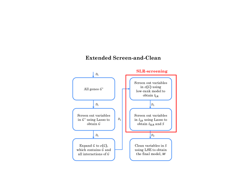
For the determination of in Step-1 of ESC, in Wu et al. (2010) they use cross-validation. Later, Liu, Roeder and Wasserman (2010) introduce StARS (Stability Approach to Regularization Selection) for selection, and this selection criterion is adopted in the R code of Screen & Clean (available at http://wpicr.wpic.pitt.edu/WPICCompGen/). Note that the intercept will be included in the model all the time. Note also that the proposed ESC is exactly the same with Wu’s SC, except SLR-screening is implemented in Step-2 instead of Lasso screening. See Figure 1 for the flowchart of ESC.
4 Simulation Studies
Our simulation studies are based on the design considered in Wu et al. (2010) with some extensions. In each simulated dataset, we generated genotype and trait values of individuals. For genotypes, we generated 1000 SNPs, with , from a discretization of normal random variable satisfying and . The 1000 SNPs can be grouped into 5-SNP blocks, with which SNPs from different blocks are independent and SNPs within the same block are correlated with . Conditional on , we generate using the following 4 models, where is the effect size and :
-
M1:
.
-
M2:
.
-
M3:
, for and for .
-
M4:
, where we randomly generate with and for , and for .
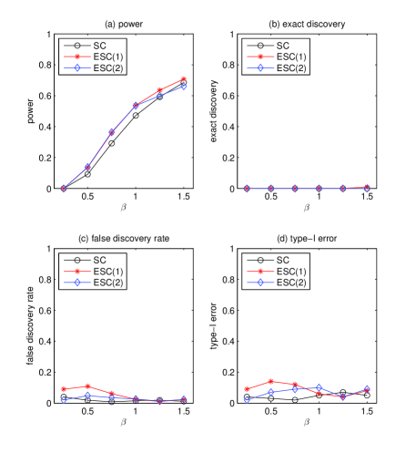
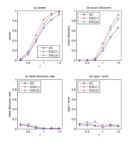
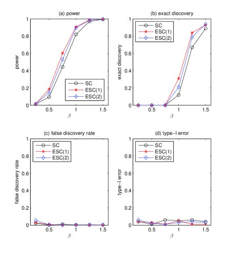
To compare the performances, let denote the index set of nonzero coefficients of the true model, and let be the estimated model. Define the power to be , the exact discovery to be , the false discovery rate (FDR) to be , and the type-I error to be . These quantities are reported with 100 replicates for each model.
Simulation results under different model settings are placed in Figures 2-5. It can be seen that both ESC(1) and ESC(2) can control FDR and type-I error adequately in all settings. In the pure interaction model M1, ESC(1) is the best performer, while the performances of SC and ESC(2) are comparable. Interestingly, when the true model contains main effects (M2, Figure 3), both ESC(1) and ESC(2) do outperform SC obviously for every effect size . It indicates that conventional SC using model (1) is not able to identify main effects efficiently. We found SC procedure is more likely to wrongly filter out the true main effects in the second Lasso screening stage. However, with the low-rank screening to reduce the model size, these true main effects have higher chances to enter the final LSE cleaning and, hence, a higher power of ESC is reasonably expected. The superiority of ESC procedure can be more obviously observed under models M3-M4 (Figures 4-5), where the powers and exact discovery rates of ESC(1) and ESC(2) dominate that of SC for every effect size . One reason is that there are many significant interactions involved in M3-M4, and ESC with a low-rank model is able to correctly filter out insignificant interactions in to achieve better performances. In contrast, directly using Lasso screening does not utilize the matrix structure of . On one side, it tends to wrongly filter out significant interactions. On the other side, it tends to leave too many insignificant terms in the screening stage. Consequently, the subsequent LSE does not have enough sample size to clean the model well, and results in lower detection powers.
We note that although the rank of in models M1-M4 ranges from 6 to 8, ESC with rank-1 and rank-2 models suffice to achieve good performances. It indicates the robustness and applicability of the low-rank model (6), even with an incorrectly specified rank . Moreover, we observe that ESC(1) outperforms ESC(2) in most of the settings. Given that the aim of low-rank screening in SLR-screening is to reduce the model size, a good approximation of is capable to remove non-important terms. In contrast, while the rank-2 model approximates more precisely, it also requires more parameters in model fitting. With limited sample size, the gain in approximation accuracy from rank-2 model cannot compensate the loss in estimation efficiency and, hence, ESC(2) may not have a better performance than ESC(1) does. See also Remark 3 for the discussion of selecting in ESC procedure.
References
- [1]
- [2] Cook, R. D. and Ni, L. (2005). Sufficient dimension reduction via inverse regression: a minimum discrepancy approach. Journal of American Statistical Association, 100, 410-428.
- [3]
- [4] Cordell, H.J. (2009). Detecting gene-gene interactions that underlie human diseases. Nature Review Genetics, 10, 392-404.
- [5]
- [6] Fan, J. and Lv, J. (2008). Sure independnece screening for untrahigh dimenison feature selection. J. R. Statist. Soc. B, 70, 849-911.
- [7]
- [8] Henderson, H. V. and Searle, S. R. (1979). Vec and vech operators for matrices, with some uses in Jacobians and multivariate statistics. Canadian Journal of Statistics, 7, 65-81.
- [9]
- [10] Liu, H., Roeder, K. and Wasserman, L. (2010). Stability approach to regularization selection (StARS) for high dimensional graphical models. arXiv:1006.3316v1
- [11]
- [12] Magnus, J. R. and Neudecker, H. (1979). The commutation matrix: some properties and applications. Annals of Statistics, 7, 381-394.
- [13]
- [14] Meinshausen, N., Meier L., and Bühlmann, P. (2009). p-values for high-dimensional regression. JASA, 104, 1671-1681.
- [15]
- [16] Shapiro, A. (1986). Asymptotic theory of overparameterized structural models. Journal of American Statistical Association, 81, 142-149.
- [17]
- [18] Tusher, V. G., Tibshirani, R. and Chu, G. (2001). Significance analysis of micro-arrays applied to the ionizing radiation response. Proceedings of the National Academy of Sciences, 98, 5116-5121.
- [19]
- [20] Wan, X., Yang, C., Yang, Q., Xue, H., Fan, X., Tang, N.L., Yu, W. (2010). BOOST: A fast approach to detecting gene-gene interactions in genome-wide case-control studies. American Journal Human Genetics 10, 325-40.
- [21]
- [22] Wasserman, L. and Roeder, K. (2009). High-dimensional variable selection. Annals of Statistics, 37, 5A, 2178-2201.
- [23]
- [24] Wu, J., Devlin, B., Ringquist, S., Trucco, M. and Roeder, K. (2010). Screen and clean: a tool for identifying interactions in genome-wide association studies. Genetic Epidemiology, 34, 275-285.
- [25]