POLITECNICO DI TORINO

I Facoltà di Ingegneria

Corso di Laurea Magistrale in Ingegneria Aerospaziale

Tesi di Laurea Magistrale

Frequency Transient of Three-Dimensional Perturbations in Shear Flows. Similarity Properties and Wave Packets Linear Formation.

Relatore:

Prof. Daniela Tordella
 
Correlatore:
Prof. Gigliola Staffilani
(Massachusetts Institute of Technology)

Candidato:

Federico Fraternale

Marzo 2013

La Stabilità Idrodinamica e la transizione alla turbolenza sono stati oggetto di studio sin dalla fine del XIX secolo. In particolare, la discrepanza tra teoria e osservazioni sperimentali nel caso di transizioni subcritiche, ha costituito un problema complicato che ha promosso la ricerca di altri meccanismi che potessero generare la transizione, differenti da quello classico che prevede la crescita esponenziale asintotica delle onde di Tollmien-Schlichting. Nonostante il ruolo delle nonlinearità sia universalmente riconosciuto, un rinnovato interesse verso l’analisi lineare a partire dalla fine del XIX secolo è derivato dai risultati dell’analisi non modale. La possibilità di una crescita di tipo algebrico, pur significativa e anche per perturbazioni asintoticamente stabili come nel caso del flusso piano di Couette, ha aperto un nuovo scenario nello studio sulla transizione laminare-turbolento. Si osserva infatti che alcuni meccanismi, come il vortex tilting oppure il ruolo delle perturbazioni ortogonali al flusso medio, vengono riscontrati già dall’analisi lineare e tridimensionale. Inoltre si è mostrato che la crescita in energia cinetica della perturbazione è soltanto attribuibile al un meccanismo lineare.

Scopo del presente lavoro è quello di contribuire alle conoscenze attuali sull’evoluzione temporale di piccole perturbazioni tridimensinali in flussi confinati, in particolare il flusso di Couette piano, tramite l’analisi delle velocità di fase e delle frequenze. La loro evoluzione temporale è stata, ed è tuttora, poco analizzata ma contiene in realtà preziose informazioni sulla vita delle perturbazioni. I risultati ottenuti per flussi di Couette e Poiseuille mostrano la possibilità di velocità di fase diverse per le tre componenti di velocità, e soprattutto la presenza di brusche variazioni o salti nell’evoluzione temporale delle frequenze. Tali variazioni permettono di distinguere tre periodi distinti della vita della singola onda, l’Early transient, l’Intermediate transient e il Far transient, e sembrano essere correlate con l’instaurarsi di certe condizioni di self-similarità nei profili di velocità o vorticità. Tali analisi non sarebbero state possibili senza lo sviluppo di un codice di calcolo in ambiente Matlab^® basato su una soluzione semi analitica (per flussi confinati) del problema ai valori iniziali di Orr-Sommerfeld e Squire. Tale soluzione è espressa come serie di funzioni ortogonali, e la soluzione approssimata viene ottenuta applicando il metodo variazionale di Galerkin. Il codice risultante risulta decisamente vantaggioso i termini di tempi di calcolo e accuratezza. A concludere il lavoro, viene mostrata l’evoluzione lineare di disturbi localizzati in forma di pacchetti d’onda per flusso di Couette e di Strato Limite. Si evidenziano le analogie con uno scenario di transizione in presenza di spot turbolenti, le quali portano a supporre che alcune proprietà di tali strutture risiedano già nelle equazioni di governo linearizzate.

Il presente lavoro di tesi è stato in parte svolto al dipartimento di Matematica del Massachusetts Institute of Technology di Cambridge (USA), sotto la supervisione della Prof.ssa Gigliola Staffilani e tramite il progetto di mobilità extra-UE FP (Final Froject). Tale opportunità è il risultato della collaborazione tra la Prof.ssa Tordella e la Prof.ssa Staffilani.

Chapter 1       Introduction

1.1   Linear Stability and transition

The reasons for the breakdown of a laminar flow to turbulence has been one of the central issues in fluid mechanics for over a hundred years, for the many applications in the engineering, meteorology, oceanography and astrophysics. The theoretical work on transition is mainly based on the linear stability studies, which were firstly initiated in the nineteenth century by Helmholts (1868), Rayleigh and Kelvin. Reynolds (1883) dedicated to experiments on the instability of the pipe flow, and was the first to find the existence of a critical velocity (actually, the non-dimensional parameter that now brings his name, the Reynolds number) above which the transition to turbulence occurs. He observed the intermittent character of this phase as well, naming flashes the objects that we now call turbulent spots.
The formulation for the viscous stability problem is due to Orr (1907) and Sommerfeld (1908), who dedicated respectively to the Plane Couette flow and to the Plane Poiseuille flow. The Orr-Sommerfeld equation has become the basis of the modal theory of hydrodynamic stability. Many years later Tollmien (1929) calculated the first neutral eigenvalues for Plane Poiseuille flow, and Schlichting continued his work, leading to the definition of the TS-waves, whose role in the transition process is salient.
Only in the second half of the twentieth century the three-dimensional initial value problem was considered. The transient dynamics of perturbations revealed aspects that made the non-modal problem even more of interest than than the past analysis on the asymptotic states. The most important result is the presence of an algebraic behavior in the early and intermediate stages of a perturbation’s life; three main reasons for the transient growth were found: the non-orthogonality of the eigenfunctions, the possible resonance between the Orr-Sommerfeld and the Squire solutions and, for unbounded or semi-bounded flows, the presence of a continuous spectrum (see e.g. the works by Criminale and Gustavsson). The role of these mechanisms, though linear, in a transitional scenario is evident, and it is easy to understand why many efforts were made in the last two decades to investigate the conditions for “optimal growth”. Only in the recent years the role of the linear mechanisms in the subcritical transition to turbulence has been pointed out by many authors (see, among others, Henningson).

1.2   Thesis motivations and layout

The aim of the present thesis is to contribute to the actual knowledge about the transient behavior of small perturbations in channel flows. The focus will be on a quantity whose temporal evolution had not been considered in detail before: the phase velocity or, equivalently, the frequency of the components of velocity and vorticity of a perturbation. Throughout the present work, it will be shown as from the analysis of the wave frequency, three terms of a disturbance’s life can clearly be discerned. Some properties of similarity of the velocity and vorticity profiles will also be highlighted.

In Chapter 2 the mathematical background is given, and the principal equations and definitions are introduced. In Chapter 3 an analytical method to solve the Orr-Sommerfeld and Squire initial value problem is presented, together with the implementation of a Matlab^® code to obtain approximate solutions. The suggested method is verified and used for the further analysis. The focus of Chapter 4 is on the perturbation frequency and phase velocity. Numerical results are shown in terms of both the vorticity and velocity components, and similarity properties of the profiles are investigated. The last Chapter concerns the evolution of wave packets and linear spots.

Figure 1.1: Turbulent spot on a flat plate. Top: $Re=200000$, the sublayer of the spot is shown from the glass wall of the water channel, by a suspension of aluminium flakes (Cantwell et al., 1978). Bottom: $Re=400000$, the typical arrowshape angle becomes steeper; visualization by smoke in air with flood lighting, photograph by R. E. Falco, taken from the book of Dyke (1982)

Chapter 2       Mathematical background

2.1   Initial value problem for shear flows: viscous linear analysis

2.1.1   Base governing equations

In the present analysis, the flow is taken to be incompressible and the governing equations for infinitesimal disturbances in parallel flows are considered. The base flow general expression is $U_{i}=U(y)\delta_{1i}$, i.e. the streamwise direction is $x$, and it only depends on the wall-normal direction $y$. The origin of the reference system is set on the channel symmetry plane $xz$ for Plane Couette flow and Plane Poiseuille flow (PCf and PPf, in the following), and on the wall for Blasius boundary layer flow (Bbl), i.e. the flow along a flat plate with zero pressure gradient(Fig. 2.1). The equations governing the general evolution of fluid flow are the Navier-Stokes equations, that using Cartesian tensor notation read

$$\frac{\partial u_{i}}{\partial t} =-u_{j}\frac{\partial u_{i}}{\partial\tilde{x}_{j}}-\frac{\partial p}{\partial x_{i}}+\frac{1}{Re}\nabla^{2}u_{i}$$ (2.1)

$$\frac{\partial u_{i}}{\partial x_{i}} =0$$ (2.2)

supported with the typical initial and boundary conditions of the form

$$u_{i}(\mathop{}\!\bm{\mathrm{x}},0) =u^{0}_{i}(\mathop{}\!\bm{\mathrm{x}})$$ (2.3)

$$u_{i}(\mathop{}\!\bm{\mathrm{x}},t) =0\ \ \ \textrm{on walls}$$

The physical quantities u,v and w represent the velocity components, p represents the flow static pressure, and they appear in the system (2.1) in nondimensional form. For PCf and PPf the reference length is the channel semi-height h, the reference velocity is assumed to be the medium wall velocity $U_{p}=(U^{+}-U^{-})/2$ for PCf, and the centeline velocity $U_{CL}$ for PPf. For Bbl, the velocity scale is the freestream velocity $U_{\infty}$ and the length scale is the boundary layer displacement thickness $\delta^{*}$, which takes the following expression, as exact solution of the Blasius equation (Schlichting, 1979, p. 141):

$$\delta^{*}=1.7208\sqrt{\frac{\nu x}{U_{\infty}}}\ \ \ (displacement\ thickness)$$ (2.4)

The approximate expression for the geometric thickness, defined as the distance for which $u=0.99U_{\infty}$, is found to be

$$\delta_{0.99}=4.91\sqrt{\frac{\nu x}{U_{\infty}}}\ \ \ (geometric\ thickness)$$ (2.5)

So the following definitions for the Reynolds number will be considered

$$Re=\frac{U_{p}h}{\nu}\ \ \textrm{Plane Couette flow}\hskip 22.76219ptRe=\frac{U_{CL}h}{\nu}\ \ \textrm{Plane Poiseuille flow}$$ (2.6)

$$Re=\frac{U_{\infty}\delta^{*}}{\nu}\ \ \textrm{Blasius boundary layer}$$ (2.7)

where $\nu$ is the kinematic viscosity. The evolution equation for the disturbances can be obtained by splitting the flow in two components, the Base flow $(U_{i}(y),P(y))$ and the perturbed state $(\tilde{u}_{i}(\mathbf{x},t),\tilde{p}(\mathbf{x},t))$ so that the complete fluid field can be written as $u_{i}=U_{i}+\tilde{u}_{i}$ and $p=P+\tilde{p}$. The nonlinear disturbance equations read

$$\frac{\partial\tilde{u}_{i}}{\partial t} =-U_{j}\frac{\partial\tilde{u}_{i}}{\partial x_{j}}-\tilde{u}_{j}\frac{\partial U_{i}}{\partial x_{j}}-\frac{\partial\tilde{p}}{\partial x_{i}}+\frac{1}{Re}\nabla^{2}\tilde{u}_{i}-\tilde{u}_{j}\frac{\partial\tilde{u}_{i}}{\partial x_{j}}$$ (2.8)

$$\frac{\partial\tilde{u}_{i}}{\partial x_{i}} =0$$ (2.9)

toghether with the appropriate initial and boundary conditions.

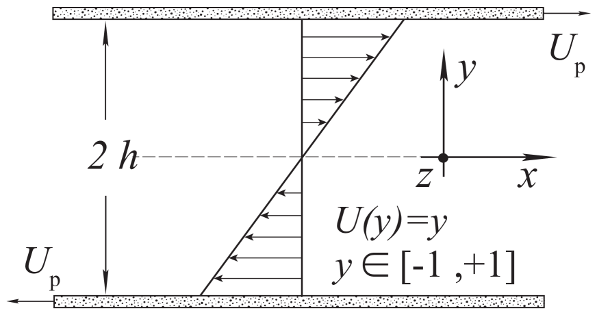
(a) PCf: $L_{ref}=h$, $U_{ref}=U_{p}$

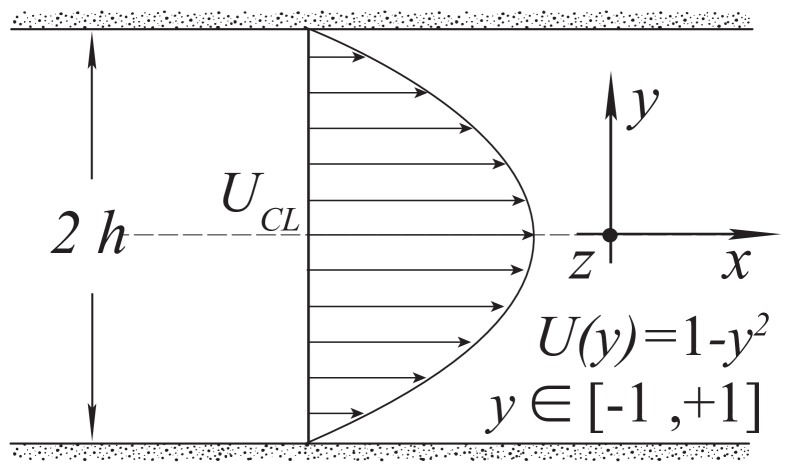
(b) PPf: $L_{ref}=h$, $U_{ref}=U_{CL}$

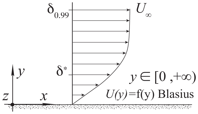
(c) Bbl: $L_{ref}=\delta^{*}$, $U_{ref}=U_{\infty}$

Figure 2.1: Flow schemes: reference quantities, base flow and reference systems.

2.1.2   Linearized perturbative equations

Considering the $x$ reference axis oriented as the base flow streamwise direction, so that it assumes the general expression $U_{i}=U(y)\delta_{1i}$, the complete velocity field becomes $\mathbf{u}=(U+\tilde{u},\tilde{v},\tilde{w})$. In particular, for PCf $U(y)=y$, and for Bbl the base velocity profile is tabulated in self-similar coordinates (Rosenhead, 1963, Chap. V). Introducing the mean velocity profile and assuming small perturbations, the following linear equations can be written, as shown by Schmid & Henningson (2001) and Criminale (2003):

$$\frac{\partial\tilde{u}}{\partial x}+\frac{\partial\tilde{v}}{\partial y}+\frac{\partial\tilde{w}}{\partial z}=0$$ (2.10)

$$\frac{\partial\tilde{u}}{\partial t}+U\frac{\partial\tilde{u}}{\partial x}+\tilde{v}\frac{dU}{dy}=-\frac{\partial\tilde{p}}{\partial x}+\frac{1}{Re}\nabla^{2}\tilde{u}$$ (2.11)

$$\frac{\partial\tilde{v}}{\partial t}+U\frac{\partial\tilde{v}}{\partial x}=-\frac{\partial\tilde{p}}{\partial y}+\frac{1}{Re}\nabla^{2}\tilde{v}$$ (2.12)

$$\frac{\partial\tilde{w}}{\partial t}+U\frac{\partial\tilde{w}}{\partial x}=-\frac{\partial\tilde{p}}{\partial z}+\frac{1}{Re}\nabla^{2}\tilde{w}$$ (2.13)

Taking the divergence of the linearized momentum equations (2.11), (2.12), (2.13), and using the continuity equation (2.10), an equation for the fluctuating pressure can be obtained and used to eliminate the pressure terms, in combination with (2.12), leading to the following equation for the wall-normal velocity:

$$\bigg{[}(\frac{\partial}{\partial t}+U\frac{\partial}{\partial x})\nabla^{2}-\frac{d^{2}U}{dy^{2}}\frac{\partial}{\partial x}-\frac{1}{Re}\nabla^{4}\bigg{]}\tilde{v}=0$$ (2.14)

To completely describe the three-dimensional flow field, a second equation is necessary, and it is convenient to write an equation for wall-normal vorticity, defined as $\tilde{\eta}=\frac{\partial\tilde{u}}{\partial z}-\frac{\partial\tilde{w}}{\partial x}$

$$\bigg{[}\frac{\partial}{\partial t}+U\frac{\partial}{\partial x}-\frac{1}{Re}\nabla^{2}\bigg{]}\tilde{\eta}=-\frac{dU}{dy}\frac{\partial\tilde{v}}{\partial z}$$ (2.15)

The quantity $\tilde{\Gamma}$ is then defined as $\tilde{\Gamma}=\nabla^{2}\tilde{v}$, so that the system becomes

$$\tilde{\Gamma} =\nabla^{2}\tilde{v}$$ (2.16)

$$\bigg{[}\frac{\partial}{\partial t}+U\frac{\partial}{\partial x}-\frac{1}{Re}\nabla^{2}\bigg{]}\tilde{\Gamma} =\frac{d^{2}U}{dy^{2}}\frac{\partial\tilde{v}}{\partial x}$$ (2.17)

$$\bigg{[}\frac{\partial}{\partial t}+U\frac{\partial}{\partial x}-\frac{1}{Re}\nabla^{2}\bigg{]}\tilde{\eta} =-\frac{dU}{dy}\frac{\partial\tilde{v}}{\partial z}$$ (2.18)

The perturbations are Fourier transformed in x and z directions: two real wavenumbers, $\alpha$ and $\beta$ are introduced along the $x$ and $z$ coordinates, respectively. The generic quantity $\hat{f}$ is hence expressed as

$$\hat{f}(y,t;\alpha,\beta)=\int_{-\infty}^{+\infty}\int_{-\infty}^{+\infty}\tilde{f}(x,y,z,t)e^{-i\alpha x-i\beta z}dxdz$$ (2.19)

The system can now be written in the following form

$$\frac{\partial^{2}\hat{v}}{\partial y^{2}}-k^{2}\hat{v}=\tilde{\Gamma}$$ (2.20)

$$\frac{\partial\hat{\Gamma}}{\partial t}=-ikcos(\phi)U\hat{\Gamma}+ikcos(\phi)\frac{d^{2}U}{dy^{2}}\hat{v}+\frac{1}{Re}\bigg{(}\frac{\partial^{2}\hat{\Gamma}}{\partial y^{2}}-k^{2}\hat{\Gamma}\bigg{)}$$ (2.21)

$$\frac{\partial\hat{\eta}}{\partial t}=-ikcos(\phi)U\hat{\eta}-iksin(\phi)\frac{d^{2}U}{dy^{2}}\hat{v}+\frac{1}{Re}\bigg{(}\frac{\partial^{2}\hat{\eta}}{\partial y^{2}}-k^{2}\hat{\eta}\bigg{)}$$ (2.22)

where $\phi=tan^{-1}(\beta/\alpha)$ is the perturbation obliquity angle, and $k=\sqrt{\alpha^{2}+\beta^{2}}$ is the polar wavenumber. The following boundary conditons applies in the wavenumber space, respectively for Bbl and PCf:

$$\hat{v}(y=\pm 1,t)=\frac{\partial\hat{v}}{\partial y}(y=\pm 1,t)=\hat{\eta}(y=\pm 1,t)=0\ \ \ \$$ (2.23)

$$\hat{v}(y\to+\infty,t)=\frac{\partial\hat{v}}{\partial y}(y\to+\infty,t)=\hat{\eta}(y\to+\infty,t)=0$$ (2.24)

The streamwise velocity $\hat{u}$ and the spanvise velocity $\hat{w}$ can be recovered from the following expressions

$$\hat{u}=\frac{i}{k^{2}}(\alpha\frac{\partial\hat{v}}{\partial y}-\beta\hat{\eta})$$ (2.25)

$$\hat{w}=\frac{i}{k^{2}}(\beta\frac{\partial\hat{v}}{\partial y}+\alpha\hat{\eta})$$ (2.26)

2.1.3   Energy amplification factor

In order to quantify the growth of the perturbations, a natural choice is the kinetic energy density, defined as

$$e(t;\alpha,\beta) =\frac{1}{2}\int_{y_{a}}^{y_{b}}\big{(}|\hat{u}|^{2}+|\hat{v}|^{2}+|\hat{w}|^{2}\big{)}dy$$ (2.27)

$$=\frac{1}{2k^{2}}\int_{y_{a}}^{y_{b}}\bigg{(}\bigg{|}\frac{\partial\hat{v}}{\partial y}\bigg{|}^{2}+k^{2}|\hat{v}|^{2}+|\hat{\eta}|^{2}\bigg{)}dy$$ (2.28)

where $y_{a}$ and $y_{b}$ are the limits of the domain. As a disturbance measure, the proper quantity is the energy amplification factor, $G$, defined as the kinetic energy density normalized with respect to its initial value (Criminale et al., 1997; Lasseigne et al., 1999)

$$G(t;\alpha,\beta)=\frac{e(t;\alpha,\beta)}{e(t=0;\alpha,\beta)}$$ (2.29)

the temporal growth rate of the kinetic energy $r$ is then introduced to evaluate the beginning of the exponential asymptotic period, when $dr/dt\to 0$

$$r(t;\alpha,\beta)=\frac{log|e(t;\alpha,\beta)|}{2t},t>0$$ (2.30)

Chapter 3       Wave transient analysis: an eigenfunction expansion solution method

3.1   Introduction

In the present chapter an analytical solution to the Orr-Sommerfeld and Squire initial value problem (eq. 3.1 and 3.2) is researched for channel flows, aiming to a better understanding of the early and intermediate terms of a perturbation’s life. As a starting point, the IVP in the normal-velocity and normal-vorticity form is considered

$$\frac{\partial}{\partial t}\frac{\partial^{2}\hat{v}}{\partial y^{2}}-k^{2}\frac{\partial\hat{v}}{\partial t}+i\alpha U(y)\frac{\partial^{2}\hat{v}}{\partial y^{2}}-i\alpha k^{2}U(y)\hat{v}-i\alpha U^{\prime\prime}(y)\hat{v}-\frac{1}{Re}\bigg{(}\frac{\partial^{4}\hat{v}}{\partial y^{4}}-2k^{2}\frac{\partial^{2}\hat{v}}{\partial y^{2}}+k^{4}\hat{v}\bigg{)}=0$$ (3.1)

$$\frac{\partial\hat{\eta}}{\partial t}+i\alpha U(y)\hat{\eta}-\frac{1}{Re}\bigg{(}\frac{\partial^{2}\hat{\eta}}{\partial y^{2}}-k^{2}\hat{\eta}\bigg{)}=-i\beta U(y)^{\prime}\hat{v}$$ (3.2)

$$\hat{v}(y=\pm 1,t)=\frac{\partial\hat{v}}{\partial y}(y=\pm 1,t)=\hat{\eta}(y=\pm 1,t)=0$$ (3.3)

$$\hat{v}(y,t=0)=\hat{v}_{0}(y)\ \ \ \ \hat{\eta}(y,t=0)=\hat{\eta}_{0}(y)$$ (3.4)

where the prime symbol indicates a total derivative along $y$. The evolution of the wall-normal velocity $\hat{v}$ is described by the Orr-Sommerfeld PDE (3.1), which is of fourth order in the spatial coordinate $y$ and homogeneous, with homogeneous boundary conditions. The Squire equation (3.2) is inhomogeneous and the forcing term $-i\beta U(y)^{\prime}\hat{v}$ is known as vortex tilting, being the product of the main vorticity in the spanwise direction ($\Omega_{z}=-U^{\prime}$) and the perturbation velocity $\hat{v}$. This term is responsible of the increase of the normal vorticity, for three-dimensional perturbations (see Criminale et al., 1997).
About the initial conditions, the following will be used in the present work

$$\hat{v}_{0}(y)=(1-y^{2})^{2}\ \ \ \hat{\eta}_{0}(y)=0\hskip 28.45274ptSymmetrical$$ (3.5)

$$\hat{v}_{0}(y)=y(1-y^{2})^{2}\ \ \ \hat{\eta}_{0}(y)=0\hskip 28.45274ptAntisymmetrical$$ (3.6)

It is known that for bounded flows all eigenvalues of the Orr-Sommerfeld and Squire ODE are discrete and infinite in number and that the eigensolutions of the problem form a complete set as proved by Schensted (1960) and DiPrima & Habetler (1969). For unbounded or semi-bounded flows (as the Wake or the Boundary layer flows) Miklavčič & Williams (1982) and Miklavčič (1983) proved that if the base flow decays in an exponential way, then only a finite number of eigenvalues exists and a continuum is present, while if the decay is algebraic there exists a infinite discrete set (without the continuum).

The focus of this chapter is on channel flows. Most of the studies in the past century deal with the modal analysis. About the Orr-Sommerfeld ODE, it is possible to express the solution as a generalized Fourier series once a base of orthogonal functions is found, and variational or Galerkin methods can be applied to provide very accurate approximations when a finite number of trial functions are used.
The Orr-Sommerfeld and Squire modes can be used to express the solution (see Schmid & Henningson, 2001), however it was shown that some sets of normal functions can give better results in terms of accuracy and computational cost. Orszag (1971) solved the Orr-Sommerfeld ODE numerically using expansions in Chebyshev polynomials and used the Lanczos’s tau method to determine the series coefficients. He showed that this series gives the highest convergence rate, since the error after $N$ terms is smaller than any power of $N^{-1}$. Before him, Dolph & Lewis (1958) were the first applying a Galerkin method to obtain the coefficients (reduction to a system of $N$ algebraic equations), together with the $QR$ algorithm. They used normal functions that guarantee a $N^{4}$ rate. Gallagher & Mercer (1962) used the Chandrasekhar functions, adopted in the present work as well, which provide a rate of convergence of $N^{5}$.

About the solution of the initial value problem, there is no conceptual difficulty in using the eigensolutions of the Orr-Sommerfeld and Squire ODE system but, as outlined in Drazin & Reid (2004), this requires the solution of the adjoint differential equation.
In the first part of this chapter an eigenfunction expansion method for the initial value problem (3.1)-(3.2) is proposed; the method does not involve the eigensolutions to the Orr-Sommerfeld and Squire ODE system, and the approximate time-dependent coefficients are obtained with the variational minimization principle. The two PDEs are then reduced to a system of $N$ ODEs. A Matlab^® code is implemented and verified and afterwards used for the analysis of Chapter 4, whose focus will be on the wave frequency and velocity profiles.

3.2   Solution to $\hat{v}$ equation

3.2.1   Choice of a base of orthogonal functions

The solution of (3.1) can be expressed as a generalized Fourier expansion, with time-dependent coeffcients:

$$\hat{v}(y,t)=\sum_{n=1}^{\infty}c_{n}(t)X_{n}(y)\ \ \ \ y\in[-1,1]$$ (3.7)

where $X_{n}(y)$ are orthogonal functions, and the following inverse transform applies (see Strauss, 1992):

$$c_{n}(t)=\frac{\int_{-1}^{1}\hat{v}(y,t)X_{n}(y)\mathop{}\!\mathrm{d}y}{\int_{-1}^{1}X_{n}(y)X_{n}(y)\mathop{}\!\mathrm{d}y}$$ (3.8)

Since in the initial value problem both the initial condition and the boundary conditions need to be imposed, it is worthwhile to consider functions that satisfy the boundary conditions of the problem considered. Moreover, note that the coefficients $c_{n}$ of the series are in general complex, since $\hat{v}$ is complex-valued and the spatial modes are considered as real. The particular orthogonal functions which we use are those defined by the following fourth order eigenvalue problem satisfying the same boundary conditions of the original equation. This choice for the simplified problem is not the only possible but revealed to be appropriate; note that this model equation is contained in the diffusive part of the PDE (3.1)

$$\frac{\partial^{4}X(y)}{\partial y^{4}}=\lambda^{4}X(y)\ \ \ \ \ y\in[-1,1]$$ (3.9)

$$X(y=\pm 1)=0\ \ \ \ \frac{\partial X}{\partial y}(y=\pm 1)=0$$ (3.10)

A solution to this problem is obtained considering sines, cosines, hyperbolic sines and hyperbolic cosines (see appendix A.1 for the complete solution). Two different sets of eigenvalues and the corresponding eigenfunctions are found, respectively odd and even, by numerically solving the following transcendental equations

$$tan(\lambda_{n})-tanh(\lambda_{n})=0\ \ \ (odd\ set)$$ (3.11)

$$tan(\lambda_{n})+tanh(\lambda_{n})=0\ \ \ (even\ set)$$ (3.12)

The corresponding normalized eigenfunctions (Fig. 3.1) are

$$X_{n}=\frac{1}{\sqrt{2}}\bigg{[}\frac{sinh(\lambda_{n}y)}{sinh(\lambda_{n})}-\frac{sin(\lambda_{n}y)}{sin(\lambda_{n})}\bigg{]}\hskip 28.45274pt{n=1,3,5..,N-1}\ \ \ (odd\ set)$$ (3.13)

$$X_{n}=\frac{1}{\sqrt{2}}\bigg{[}\frac{cosh(\lambda_{n}y)}{cosh(\lambda_{n})}-\frac{cos(\lambda_{n}y)}{cos(\lambda_{n})}\bigg{]}\hskip 28.45274pt{n=2,4,6..,N}\ \ \ \ \ (even\ set)$$ (3.14)

Similar functions, in a different domain, have been used by Chandrasekhar (1961, app. V), in the study of the circular Couette flow between coaxial cylinders, and by Gallagher & Mercer (1962) to solve the Orr-Sommerfeld ODE.

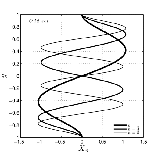
Figure 3.1: The basis eigenfunctions

Since the imaginary and the real part of the solution $\hat{v}$ usually have opposite parity, independently on the initial condition, both the odd and the even set are necessary to completely describe the problem and obtain the correct result.
In the following paragraphs a compact notation for the space derivatives is introduced. In order to simplify the reading, the $y$-derivatives will be indicated with a subscript. The temporal derivatives will be indicated explicitly or with a dot.

3.2.2   Weak formulation and approximate solution to $\hat{v}$ equation by Galerkin method

Substituting the expansion (3.7) in $\hat{v}$ equation (3.1) yields

$$\begin{split}0&=\sum_{n=1}^{\infty}\frac{\mathrm{d}}{\mathrm{d}t}c_{n}(t)X_{n_{yy}}-k^{2}\sum_{n=1}^{\infty}\frac{\mathrm{d}}{\mathrm{d}t}c_{n}(t)X_{n}+i\alpha U(y)\sum_{n=1}^{\infty}c_{n}(t)X_{n_{yy}}\\ &-i\alpha k^{2}U(y)\sum_{n=1}^{\infty}c_{n}(t)X_{n}-i\alpha\frac{\mathop{}\!\mathrm{d}^{2}U(y)}{\mathop{}\!\mathrm{d}y^{2}}\sum_{n=1}^{\infty}c_{n}(t)X_{n}-\frac{1}{Re}\sum_{n=1}^{\infty}c_{n}(t)X_{n_{yyyy}}\\ &+\frac{2k^{2}}{Re}\sum_{n=1}^{\infty}c_{n}(t)X_{n_{yy}}-\frac{k^{4}}{Re}\sum_{n=1}^{\infty}c_{n}(t)X_{n}\end{split}$$ (3.15)

The above expression represents an exact form. If only a finite number of modes is considered, the equation is not satisfied exactly, so a residual $\epsilon$ (dependent on the choice of the functions $X_{n}$) appears at the left hand side

$$\begin{split}\epsilon(y,t;\ \alpha,\ \beta)&=\sum_{n=1}^{N}\frac{\mathrm{d}}{\mathrm{d}t}c_{n}(t)X_{n_{yy}}-k^{2}\sum_{n=1}^{N}\frac{\mathrm{d}}{\mathrm{d}t}c_{n}(t)X_{n}+i\alpha U(y)\sum_{n=1}^{N}c_{n}(t)X_{n_{yy}}\\ &-i\alpha k^{2}U(y)\sum_{n=1}^{N}c_{n}(t)X_{n}-i\alpha\frac{\mathop{}\!\mathrm{d}^{2}U(y)}{\mathop{}\!\mathrm{d}y^{2}}\sum_{n=1}^{N}c_{n}(t)X_{n}-\frac{1}{Re}\sum_{n=1}^{N}c_{n}(t)X_{n_{yyyy}}\\ &+\frac{2k^{2}}{Re}\sum_{n=1}^{N}c_{n}(t)X_{n_{yy}}-\frac{k^{4}}{Re}\sum_{n=1}^{N}c_{n}(t)X_{n}\end{split}$$ (3.16)

Galerkin (1915) focused on the problem of minimizing the functional $\epsilon$, so his method consists of a variational approach (see also Chandrasekhar, 1961, p. 27-32). He showed that the best approximation of the solution is obtained when the error is orthogonal to the space of the linearly independent trial functions $X_{n}$ with $n={1,2,..N}$. In this context, given two functions $u(y)$ and $v(y)$ with $y\in\ \Omega=[-1,\ 1]$, the following definition of scalar product applies

$$\langle u,v\rangle\overset{def}{=}\int_{\Omega}u\cdot v\mathop{}\!\mathrm{d}y$$ (3.17)

so, using the above notation, the Galerkin orthogonality condition can be expressed as

$$\langle\epsilon,X_{m}\rangle=0\ \hskip 42.67912ptm=1,2,...,N$$ (3.18)

Substituting $\epsilon$ with its expression (3.16), inverting the integral and the sum signs, and taking the time dependent coefficients out of the integral sign, leads to the following system of equations

$$\begin{split}0&=\sum_{n=1}^{N}\frac{\mathrm{d}}{\mathrm{d}t}c_{n}(t)\langle X_{n_{yy}},X_{m}\rangle-k^{2}\sum_{n=1}^{N}\frac{\mathrm{d}}{\mathrm{d}t}c_{n}(t)\langle X_{n},X_{m}\rangle+i\alpha\sum_{n=1}^{N}c_{n}(t)\langle U(y)X_{n_{yy}},X_{m}\rangle\\ &-i\alpha k^{2}\sum_{n=1}^{N}c_{n}(t)\langle U(y)X_{n},X_{m}\rangle-i\alpha\sum_{n=1}^{N}c_{n}(t)\langle\frac{\mathop{}\!\mathrm{d}^{2}U(y)}{\mathop{}\!\mathrm{d}y^{2}}X_{n}X_{m}\rangle-\frac{1}{Re}\sum_{n=1}^{N}c_{n}(t)\langle X_{n_{yyyy}},X_{m}\rangle\\ &+\frac{2k^{2}}{Re}\sum_{n=1}^{N}c_{n}(t)\langle X_{n_{yy}},X_{m}\rangle-\frac{k^{4}}{Re}\sum_{n=1}^{N}c_{n}(t)\langle X_{n},X_{m}\rangle\hskip 42.67912ptn,\ m=1,2,3,...,N\end{split}$$ (3.19)

The original partial differential equation is now reduced to a system of $N$ ordinary differential equations of the first order, where the time dependent coefficients $c_{n}(t)$ are the only unknown. The scalar products can be evaluated analytically or computed by numerical integration and take the following expressions

$$D_{m,n}=\langle X_{n},X_{m}\rangle=\delta_{m,n}$$ (3.20)

$$S_{m,n}=\langle X_{n_{yy}},X_{m}\rangle=$$ (3.21)

$$=\begin{cases}+4\frac{\lambda_{n}^{2}\lambda_{m}^{2}}{\lambda_{n}^{4}-\lambda_{m}^{4}}(\lambda_{n}\gamma_{n}-\lambda_{m}\gamma_{m})&\mbox{if }(n+m)\mbox{ is even, }n\neq m\\ 0&\mbox{if }(n+m)\mbox{ is odd}\\ -\lambda_{n}^{2}\gamma_{n}^{2}+\lambda_{m}\gamma_{m}&\mbox{if }n=m\end{cases}$$

$$F_{m,n}=\langle X_{n_{yyyy}},X_{m}\rangle=\lambda_{n}^{4}\delta_{m,n}$$ (3.22)

where

$$\gamma_{n}=\frac{cosh(2\lambda_{n})-cos(2\lambda_{n})}{sinh(2\lambda_{n})-sin(2\lambda_{n})}\hskip 28.45274pt\lim_{n\to\infty}\gamma_{n}=1$$ (3.23)

For Plane Couette flow, in all the present work the following expression of the base flow will be considered

$$U(y)=y$$ (3.24)

so that the other integrals take the expressions

$$U^{(1)}_{m,n}=\langle U(y)X_{n_{yy}},X_{m}\rangle=$$ (3.25)

$$=\begin{cases}0&\mbox{if }(n+m)\mbox{ is even, }n\neq m\\ 4\frac{\lambda_{n}^{2}\lambda_{m}^{2}}{\lambda_{n}^{4}-\lambda_{m}^{4}}(\lambda_{n}\gamma_{n}-\lambda_{m}\gamma_{m}-1)-8\frac{\gamma_{n}^{4}+\gamma_{m}^{4}}{(\lambda_{n}^{4}-\lambda_{m}^{4})^{2}}\lambda_{n}^{2}\lambda_{m}^{2}&\mbox{if }(n+m)\mbox{ is odd}\\ 0&\mbox{if }n=m\end{cases}$$

$$U^{(2)}_{m,n}=\langle U(y)X_{n},X_{m}\rangle=$$ (3.27)

$$=\begin{cases}0&\mbox{if }(n+m)\mbox{ is even, }n\neq m\\ 16\frac{\lambda_{n}^{3}\lambda_{m}^{3}\gamma_{n}\gamma_{m}}{(\lambda_{n}^{4}-\lambda_{m}^{4})^{2}}&\mbox{if }(n+m)\mbox{ is odd}\\ 0&\mbox{if }n=m\end{cases}$$

$$U^{(3)}_{m,n}=\langle\frac{\mathop{}\!\mathrm{d}^{2}U(y)}{\mathop{}\!\mathrm{d}y^{2}}X_{n},X_{m}\rangle=0\ \ \ \ \forall\ n,m$$ (3.28)

It is convenient to express the ODEs system (3.19) in a more compact notation: in the following, vectors will be indicated either explicitly using braces or with bold lower case letters; matrices will be indicated with bold capital letters; constants with roman capital letters and physical parameters in italic. The system can be written as

$$\underbrace{\big{(}\mathop{}\!\bm{\mathrm{S}}-k^{2}\mathop{}\!\bm{\mathrm{D}}\big{)}}_{\mathop{}\!\bm{\mathrm{H}}}\mathop{}\!\bm{\mathrm{\dot{c}}}-\underbrace{\big{(}\ -i\alpha\mathop{}\!\bm{\mathrm{U^{(1)}}}+i\alpha k^{2}\mathop{}\!\bm{\mathrm{U^{(2)}}}+i\alpha\mathop{}\!\bm{\mathrm{U^{(3)}}}+\frac{1}{Re}\mathop{}\!\bm{\mathrm{F}}-\frac{2k^{2}}{Re}\mathop{}\!\bm{\mathrm{S}}+\frac{k^{4}}{Re}\mathop{}\!\bm{\mathrm{D}}\big{)}}_{\mathop{}\!\bm{\mathrm{G}}}\mathop{}\!\bm{\mathrm{c}}=0$$ (3.29)

$$\mathop{}\!\bm{\mathrm{H}}\mathop{}\!\bm{\mathrm{\dot{c}}}-\mathop{}\!\bm{\mathrm{G}}\mathop{}\!\bm{\mathrm{c}}=0$$ (3.30)

where $\mathop{}\!\bm{\mathrm{D}}=[D_{m,n}]$ etc., i.e. the element $D_{m,n}$ is placed at the $n^{th}$ column and at the $m^{th}$ row of the matrix. $\mathop{}\!\bm{\mathrm{H}}$ is invertible, so denoting $\mathop{}\!\bm{\mathrm{A}}=\mathop{}\!\bm{\mathrm{H}}^{-1}\mathop{}\!\bm{\mathrm{G}}$ yields

$$\mathop{}\!\bm{\mathrm{\dot{c}}}-\mathop{}\!\bm{\mathrm{A}}\mathop{}\!\bm{\mathrm{c}}=0$$ (3.31)

The general solution to the ODEs system (3.31) in the case of matrix $\mathop{}\!\bm{\mathrm{A}}$ having $N$ distinct eigenvalues $\mu_{i}$ (either real or complex, see Zill & Cullen, 2005), reads

$$\mathop{}\!\bm{\mathrm{c}}(t)=\mathrm{K_{1}}\mathop{}\!\bm{\mathrm{l}}_{1}e^{\mu_{1}t}+\mathrm{K_{2}}\mathop{}\!\bm{\mathrm{l}}_{2}e^{\mu_{2}t}+\ldots+\mathrm{K_{N}}\mathop{}\!\bm{\mathrm{l}}_{N}e^{\mu_{N}t}$$ (3.32)

where $\mathop{}\!\bm{\mathrm{l}}_{i}$ are the eigenvectors corresponding to $\mu_{i}$ and $\mathrm{K_{i}}$ are constants to be determined by imposing the initial condition, or alternatively using the Matrix Exponential notation

$$\mathop{}\!\bm{\mathrm{c}}(t)=e^{\mathop{}\!\bm{\mathrm{A}}t}\{K_{i}\}$$ (3.33)

The coefficients at the initial time, $\mathop{}\!\bm{\mathrm{c_{0}}}$, can be obtained from the inverse transformation (3.8) since the initial condition $\hat{v}(t=0)$ is known, so finally the solution is get by solving the algebraic system

$$\mathop{}\!\bm{\mathrm{c_{0}}}=\mathrm{K_{1}}\mathop{}\!\bm{\mathrm{l}}_{1}+\mathrm{K_{2}}\mathop{}\!\bm{\mathrm{l}}_{2}+........+\mathrm{K_{N}}\mathop{}\!\bm{\mathrm{l}}_{N}$$ (3.34)

$$\mathop{}\!\bm{\mathrm{h_{0}}}=\{K_{i}\}=\mathop{}\!\bm{\mathrm{L}}^{-1}\mathop{}\!\bm{\mathrm{c_{0}}}$$ (3.35)

where $\mathop{}\!\bm{\mathrm{h}}(t)=\mathop{}\!\bm{\mathrm{L}}^{-1}\mathop{}\!\bm{\mathrm{c}}(t)$, and $\mathop{}\!\bm{\mathrm{L}}$ is the matrix whose columns are the eigenvectors $\mathop{}\!\bm{\mathrm{l}}_{i}$. Their linear independence ensures that $\mathop{}\!\bm{\mathrm{L}}$ is invertible.

3.3   Solution to the forced $\hat{\eta}$ equation

3.3.1   Choice of a base of orthogonal functions

Following the same procedure of §3.2.1, we now focus on the normal-vorticity equation (3.2), which is forced by the solution $\hat{v}$ of the Orr-Sommerfeld PDE equation (3.1). Together with the non-orthogonality of the Orr-Sommerfeld differential operator, a resonance phenomenon has been pointed out as one of the reasons for large energy transient growths, if there is sufficient wave obliquity (see Gustavsson, 1991). In order to solve the $\hat{\eta}$ equation a set of normal functions different from the one adopted in §3.2.1 is needed, since the second order PDE only requires $\hat{\eta}$ to vanish at the boundaries, but not its first derivative . The simplest choice for the basis functions, here adopted, is the following

$$Y_{n}=sin(\xi_{n}y)\hskip 42.67912ptn=1,3,5,...N-1\ \ (odd\ set)$$ (3.36)

$$Y_{n}=cos(\xi_{n}y)\hskip 42.67912ptn=2,4,6,...N\ \ \ (even\ set)$$ (3.37)

where

$$\xi_{n}=\frac{(n+1)\pi}{2}\hskip 28.45274ptn=1,3,5,...N-1\ \ (odd\ set)$$ (3.38)

$$\xi_{n}=\frac{(n-1)\pi}{2}\hskip 28.45274ptn=2,4,6,...N\ \ \ (even\ set)$$ (3.39)

Also in this case, note that two sets of eigenfunctions are put together to form a unique set, since both are necessary to completely describe the complex-valued normal vorticity. The general solution is then obtained as the sum of a particular solution $\hat{\eta}_{p}$ and the solution to the corresponding homogeneous equation $\hat{\eta}_{h}$

$$\hat{\eta}(y,t)=\hat{\eta}_{h}(y,t)+\hat{\eta}_{p}(y,t)$$ (3.40)

3.3.2   Weak formulation and approximate solution to $\hat{\eta}$ equation by Galerkin method

Considering the complete equation (3.2), we proceed as done for the normal-velocity and expand the solution as follows

$$\hat{\eta}(y,t)=\sum_{n=1}^{\infty}b_{n}(t)Y_{n}(y)$$ (3.41)

Substituting, the equation reads

$$\begin{split}&\sum_{n=1}^{\infty}\frac{\mathrm{d}}{\mathrm{d}t}b_{n}(t)Y_{n}+i\alpha U(y)\sum_{n=1}^{\infty}b_{n}(t)Y_{n}-\frac{1}{Re}\sum_{n=1}^{\infty}b_{n}(t)Y_{n_{yy}}\\ &+\frac{k^{2}}{Re}\sum_{n=1}^{\infty}b_{n}(t)Y_{n}=-i\beta\frac{\mathrm{d}U(y)}{\mathrm{d}y}\sum_{n=1}^{\infty}c_{n}(t)X_{n}(y)\end{split}$$ (3.42)

Considering a finite number $N$ of terms of the expansion and applying the Galerkin method yields

$$\begin{split}&\sum_{n=1}^{N}\frac{\mathrm{d}}{\mathrm{d}t}b_{n}(t)\langle Y_{n},Y_{m}\rangle+i\alpha\sum_{n=1}^{N}b_{n}(t)\langle U(y)Y_{n},Y_{m}\rangle-\frac{1}{Re}\sum_{n=1}^{N}b_{n}(t)\langle Y_{n_{yy}},Y_{m}\rangle\\ &+\frac{k^{2}}{Re}\sum_{n=1}^{N}b_{n}(t)\langle Y_{n},Y_{m}\rangle=-i\beta\sum_{n=1}^{N}c_{n}(t)\langle\frac{\mathrm{d}U(y)}{\mathrm{d}y}X_{n},Y_{m}\rangle\ \ \ \ n,m=1,2,3,...,N\end{split}$$ (3.43)

The scalar products can be evaluated analytically and take the following expressions

$$D^{*}_{m,n}=\langle Y_{n},Y_{m}\rangle=\delta_{m,n}$$ (3.44)

$$S^{*}_{m,n}=\langle Y_{n_{yy}},Y_{m}\rangle=-\xi_{n}^{2}\delta_{m,n}$$ (3.45)

For Plane Couette flow:

$$U^{*}_{m,n}=\langle U(y)Y_{n},Y_{m}\rangle=$$ (3.46)

$$=\begin{cases}0&\mbox{if }(n+m)\mbox{ is even, or }n=m\\ \frac{(-1)^{\frac{n+m+1}{2}}4\xi_{n}\xi_{m}}{(\xi_{n}^{2}-\xi_{m}^{2})^{2}}&\mbox{if }(n+m)\mbox{ is odd}\end{cases}$$

$$F^{*}_{m,n}=\langle\frac{\mathrm{d}U(y)}{\mathrm{d}y}X_{n},Y_{m}\rangle=$$ (3.47)

$$=\begin{cases}\frac{2\sqrt{2}\xi_{m}\xi_{n}^{2}(-1)^{\frac{m+1}{2}}}{\xi_{m}^{4}-\xi_{n}^{4}}&\mbox{if }n,m\mbox{ are odd}\\[6.0pt] \frac{2\sqrt{2}\xi_{m}\xi_{n}^{2}(-1)^{\frac{m}{2}}}{\xi_{m}^{4}-\xi_{n}^{4}}&\mbox{if }n,m\mbox{ are even}\end{cases}$$

Introducing the vector and matrix notation, the system (LABEL:system_eta_discr) reads

$$\mathop{}\!\bm{\mathrm{\dot{b}}}-\underbrace{\big{(}\ -i\alpha\mathop{}\!\bm{\mathrm{U^{*}}}+\frac{1}{Re}\mathop{}\!\bm{\mathrm{S^{*}}}-\frac{2k^{2}}{Re}\mathop{}\!\bm{\mathrm{D^{*}}}\big{)}}_{\mathop{}\!\bm{\mathrm{G^{*}}}}\mathop{}\!\bm{\mathrm{b}}=\underbrace{-i\beta\mathop{}\!\bm{\mathrm{F^{*}}}}_{\mathop{}\!\bm{\mathrm{B}}}\mathop{}\!\bm{\mathrm{c}}$$ (3.48)

$$\mathop{}\!\bm{\mathrm{\dot{b}}}-\mathop{}\!\bm{\mathrm{G^{*}}}\mathop{}\!\bm{\mathrm{b}}=\mathop{}\!\bm{\mathrm{B}}\mathop{}\!\bm{\mathrm{c}}$$ (3.49)

which is a non-homogeneuos system of $N$ ODEs. The general solution to (3.49) consists of the superposition of the solution of the homogeneous system and a particular one. Naming $\mathop{}\!\bm{\mathrm{\Phi}}(t)$ the fundamental matrix of the system ( see Zill & Cullen, 2005), then a formal expression for the general solution is

$$\mathop{}\!\bm{\mathrm{b}}(t)=\mathop{}\!\bm{\mathrm{b}}_{h}(t)+\mathop{}\!\bm{\mathrm{b}}_{p}(t)=\mathop{}\!\bm{\mathrm{\Phi}}(t)\mathop{}\!\bm{\mathrm{k}}+\mathop{}\!\bm{\mathrm{\Phi}}(t)\int_{t_{0}}^{t}\mathop{}\!\bm{\mathrm{\Phi}}^{-1}(t)\mathop{}\!\bm{\mathrm{B}}\mathop{}\!\bm{\mathrm{c}}(s)\mathop{}\!\mathrm{d}s$$ (3.50)

or, alternatively, using the Matrix Exponential form

$$\mathop{}\!\bm{\mathrm{b}}(t)=\mathop{}\!\bm{\mathrm{b}}_{h}(t)+\mathop{}\!\bm{\mathrm{b}}_{p}(t)=e^{\mathop{}\!\bm{\mathrm{G^{*}}}t}\mathop{}\!\bm{\mathrm{k}}+e^{\mathop{}\!\bm{\mathrm{G^{*}}}t}\int_{t_{0}}^{t}e^{\mathop{}\!\bm{\mathrm{-G^{*}}}t}\mathop{}\!\bm{\mathrm{B}}\mathop{}\!\bm{\mathrm{c}}(s)\mathop{}\!\mathrm{d}s$$ (3.51)

where $\mathop{}\!\bm{\mathrm{k}}$ is a vector of constants. The last expressions have the advantage that the particular integral vanishes at $t=t_{0}$, so it is easy to find the constants by imposing the initial condition. Unfortunately, a numerical evaluation of the integral can lead to non negligible errors, especially for big times, where a product of very large and very small terms occurs. In order to make the numerical computation possible, a different form for the particular solution is sought.

Particular solution $\mathop{}\!\bm{\mathrm{b}}_{p}$

Since the solution (3.32) in terms of the expansion coefficients $\mathop{}\!\bm{\mathrm{c}}(t)$ is a combination of exponentials and represents the forcing term in (3.49), the following particular solution $\mathop{}\!\bm{\mathrm{b}}_{p}$ is sought

$$b_{p_{n}}(t)=\sum_{j=1}^{N}a_{nj}e^{\mu_{j}t}$$ (3.52)

where $a_{nj}$ are constants and $\mu_{j}$ are the eigenvalues of $\mathop{}\!\bm{\mathrm{A}}$, through which the forcing term is expressed. Yields

$$\hat{\eta}_{p}(y,t)=\sum_{n=1}^{N}b_{p_{n}}(t)Y_{n}(y)$$ (3.53)

Diagonalizing the system (3.31), the coefficients of the normal-velocity result

$$\mathop{}\!\bm{\mathrm{c}}(t)=\mathop{}\!\bm{\mathrm{L}}\mathop{}\!\bm{\mathrm{h}}=\mathop{}\!\bm{\mathrm{L}}\begin{Bmatrix}h_{0_{1}}e^{\mu_{1}t}\\ h_{0_{2}}e^{\mu_{2}t}\\ \vdots\\ h_{0_{N}}e^{\mu_{N}t}\end{Bmatrix}\hskip 56.9055pt\mathop{}\!\bm{\mathrm{h_{0}}}=\mathop{}\!\bm{\mathrm{L}}^{-1}\mathop{}\!\bm{\mathrm{c}}(t=0)$$ (3.54)

Substituting the particular solution (3.52) in (3.49) and leads to

$$\frac{\mathrm{d}}{\mathrm{d}t}\begin{Bmatrix}a_{11}e^{\mu_{1}t}+\ldots a_{1N}e^{\mu_{N}t}\\ \vdots\\ a_{N1}e^{\mu_{1}t}+\ldots a_{NN}e^{\mu_{N}t}\end{Bmatrix}+\mathop{}\!\bm{\mathrm{G^{*}}}\begin{Bmatrix}a_{11}e^{\mu_{1}t}+\ldots a_{1N}e^{\mu_{N}t}\\ \vdots\\ a_{N1}e^{\mu_{1}t}+\ldots a_{NN}e^{\mu_{N}t}\end{Bmatrix}=\mathop{}\!\bm{\mathrm{B}}\mathop{}\!\bm{\mathrm{L}}\begin{Bmatrix}h_{0_{1}}e^{\mu_{1}t}\\ h_{0_{2}}e^{\mu_{2}t}\\ \vdots\\ h_{0_{N}}e^{\mu_{N}t}\end{Bmatrix}$$ (3.55)

It is straightforward to find the unknown constants $a_{nj}$ by comparing terms with the same exponential factor. This is equivalent to solve the following set of $N$ algebraic systems

$$(\mu_{j}\mathbbm{I}-\mathop{}\!\bm{\mathrm{G^{*}}})\begin{Bmatrix}a_{1j}\\ a_{2j}\\ \vdots\\ a_{Nj}\end{Bmatrix}=h_{0j}\begin{Bmatrix}B^{*}_{1j}\\ B^{*}_{2j}\\ \vdots\\ B^{*}_{Nj}\end{Bmatrix}\hskip 28.45274ptj=1,2,...N$$ (3.56)

where $\mathbbm{I}$ is the identity matrix and $B^{*}_{ij}$ are the elements of the matrix $\mathop{}\!\bm{\mathrm{B}}\mathop{}\!\bm{\mathrm{L}}$. As usual, the first subscript indicates the row and the second one indicates the column. Finally we get the matrix of coefficients column by column as

$$\begin{Bmatrix}a_{1j}\\ a_{2j}\\ \vdots\\ a_{Nj}\end{Bmatrix}=(\mu_{j}\mathbbm{I}-\mathop{}\!\bm{\mathrm{G^{*}}})^{-1}h_{0j}\begin{Bmatrix}B^{*}_{1j}\\ B^{*}_{2j}\\ \vdots\\ B^{*}_{Nj}\end{Bmatrix}\hskip 28.45274ptj=1,2,...N$$ (3.57)

Homogeneous and complete solution $\mathop{}\!\bm{\mathrm{b}}$

The homogeneous solution of (3.49) takes the same form of the of equation (3.32). Indicating with $\mu^{*}$ and $\mathop{}\!\bm{\mathrm{l}}^{*}$ respectively the eigenvalues and eigenvectors of the matrix $\mathop{}\!\bm{\mathrm{G^{*}}}$, it follows

$$\mathop{}\!\bm{\mathrm{b}}_{h}(t)=\mathrm{C_{1}}\mathop{}\!\bm{\mathrm{l}}^{*}_{1}e^{\mu_{1}^{*}t}+\mathrm{C_{2}}\mathop{}\!\bm{\mathrm{l}}^{*}_{2}e^{\mu^{*}_{2}t}+\ldots+\mathrm{C_{N}}\mathop{}\!\bm{\mathrm{l}}^{*}_{N}e^{\mu^{*}_{N}t}$$ (3.58)

Finally the complete solution is

$$\mathop{}\!\bm{\mathrm{b}}(t)=\mathrm{C_{1}}\mathop{}\!\bm{\mathrm{l}}^{*}_{1}e^{\mu_{1}^{*}t}+\mathrm{C_{2}}\mathop{}\!\bm{\mathrm{l}}^{*}_{2}e^{\mu^{*}_{2}t}+\ldots+\mathrm{C_{N}}\mathop{}\!\bm{\mathrm{l}}^{*}_{N}e^{\mu^{*}_{N}t}+\mathop{}\!\bm{\mathrm{b}}_{p}(t)$$ (3.59)

The unknown constants $\mathrm{C}_{i}$ depends on the initial condition, and can be calculated setting $t=0$ in the above expression, leading to

$$\mathop{}\!\bm{\mathrm{h^{*}_{0}}}=\{\mathrm{C}_{i}\}=\mathop{}\!\bm{\mathrm{L^{*}}}^{-1}(\mathop{}\!\bm{\mathrm{b_{0}}}-\mathop{}\!\bm{\mathrm{b_{0}}}_{p})$$ (3.60)

3.4   A Matlab^® code implementation

3.4.1   Code description

In order to verify the proposed method and to obtain the numerical solutions, a Matlab^® code has been developed and used in the further analysis. At present, it consists of two scrips: the main code solves the normal-velocity equation and calls a function to solve the normal-vorticity equation. Eventually it computes the other components of the perturbation velocity, the frequency, the energy growth factor and other quantities of interest.

The main code

The structure of the main program (main_ivp_galerkin.m) can be represented by the flowchart of Fig. 3.2. Among the other simulation parameters, the number of modes can be chosen. The corresponding eigenvalues $\lambda_{i}$ are computed by a separate script through Bisection or Newton-Raphson method, and memorized in a .mat file which can be loaded by the main program. As seen in §3.2.2, the method requires the solution to algebraic systems, so matrix inversions. In particular two inversions are needed to obtain the solution $\hat{v}$, respectively the one of the matrix $\mathop{}\!\bm{\mathrm{A}}$ and the one of the eigenvectors matrix $\mathop{}\!\bm{\mathrm{L}}$. In fact, the ill-conditioning of this matrices can influence the accuracy of the computation. In detail, the condition number of matrix $\mathop{}\!\bm{\mathrm{A}}$ does not represent a problem, while the one of matrix $\mathop{}\!\bm{\mathrm{L}}$ can reach very high values, of the order of $10^{16}$ for some parameters settings as low obliquity angles; moreover the condition number increases with increasing $N$. This fact has not been investigated in details, but is quite similar to that pointed out by Schmid & Henningson (2001). The ill-conditioning of $\mathop{}\!\bm{\mathrm{L}}$ is intrinsic, due to the non orthogonality of the Orr-Sommerfold linear operator. In order to guarantee a certain level of accuracy, the matrix inversion error is checked and compared to a threshold $tol$. The absolute pointwise error in the solution of a generic system $\mathop{}\!\bm{\mathrm{A}}\mathop{}\!\bm{\mathrm{x}}=\mathop{}\!\bm{\mathrm{b}}$ is defined as follows

$$err_{A}=\mathop{}\!\bm{\mathrm{A}}\mathop{}\!\bm{\mathrm{x}}-\mathop{}\!\bm{\mathrm{b}}$$ (3.61)

Figure 3.2: Structure of the main code main_ivp_galerkin.m.

The script computes by default the matrix inversion using the Matlab^® backslash command. Then, the norm (both $L_{2}$-norm and $L_{\infty}$-norm ) of the error is calculated and compared to the tolerance. If the threshold level is exceeded, a different method to solve the algebraic system is performed. In particular, the present code tries to approximately solve the system using the GMRES method. Both the norm of absolute and the relative error are evaluated. Even if a better method should be object of future deeper analysis, it has been observed that for every parameters combination tried, the minimum relative error is obtained using the backslash command, and its order of magnitude spans the range $10^{-12}-10^{-30}$.

The solution is obtained for every point along the space coordinate $y$ and at all time points defined by the user. Since the time evolution is analytically obtained, and since the analytical expressions of the modes is known, the accuracy of the method shouldn’t depend neither on the space nor on the time discretization. Actually, this is not exact: the computation of the coefficients $\mathop{}\!\bm{\mathrm{c_{0}}}$ is performed through numerical integration (trapezoidal rule), whose order of accuracy is $O(\Delta y^{2})$. Moreover, in the case of Plane Poiseuille flow, the scalar products $U^{(1)}_{m,n},\ U^{(2)}_{m,n}$ and $U^{*}_{m,n}$ are evaluated through numerical integration as well, so a sufficient grid spacing is required. The computation of the wave frequency or phase velocity can require very fine time grids, the motivation will be given in Chapter 4. In general, fine grids are necessary whenever a finite difference scheme for derivatives computation needs to be applied. In order to ensure an high accuracy of the computation of the initial condition, and consequently of the global solution, and at the same time allowing the user to obtain the solution only at the desired points, a separate grid is used just for the computation of the initial condition’s coefficients $\mathop{}\!\bm{\mathrm{c_{0}}}$.

The $\hat{\eta}$ solving function

The $\hat{\eta}$ equation is solved by the function solve_squire.m. The script structure is represented by the flowchart of Fig. 3.3, and is quite similar to the one of the main program. Here there is no reason to calculate the eigenvalues related to the basis functions with another script, being known their exact expression. It can be noticed that to obtain the normal vorticity the solution of the $N$ algebraic systems (3.56) is required, as well as the inversion of the matrix $\mathop{}\!\bm{\mathrm{L^{*}}}$. Depending on the choice of the simulation parameters, these matrices can be ill-conditioned so the same procedure described in the previous section is implemented. During the simulation all the error norms are displayed (about the $N$ algebraic systems (3.56), only the maximum will be shown).

Figure 3.3: Structure of the function solve_squire.m.

Also in the computation of $\hat{\eta}$, the backslash command has revealed to guarantee an high level of accuracy in all simulation performed, being all error norms of the order of $10^{-14}$ or lower.

3.4.2   Rate of Convergence

In this section, the rate of convergence of the present method to the exact solutions of the initial value problem will be investigated. The eigenfunction expansion method using the Chandrasekhar basis functions was applied to the Orr-Sommerfeld modal analysis by Gallagher & Mercer (1962). In that case, the error was shown to decrease as $1/N^{5}$ as $N\to\infty$, moreover the residue after $N$ terms of expansion was of order $1/N^{5}$.
Even if the present formulation is different in the fact that the PDEs are reduced to systems of ODEs, rather than algebraic equations, it has been verified that the convergence ratio of order $1/N^{5}$ as $N\to\infty$ is kept, and it applies at all times, for what concerns $\hat{v}$ equation. About $\hat{\eta}$ equation, the method reduces to a Fourier series expansion with time-dependent coefficients, and in this case the convergence rate is found to be only slightly different from the one of $\hat{v}$.
Both the root mean square (proportional to $L_{2}$-norm) and the maximum ($L_{\infty}$-norm) of the residual are computed. In the following, the residuals as a function of the number of modes used for the simulation are reported at two different times and two different values of the obliquity angle, for Plane Couette flow and Plane Poiseuille flow. Since the exact solution is not known, the residuals are defined as the difference between the solution and an accurate solution computed with 350 modes. The exact expression is only known at time zero, and the results have been confirmed in this case.

$$\epsilon_{a}(y,t)=|\hat{v}_{N}(y,t)-\hat{v}_{N=350}(y,t)|$$ (3.62)

$$rms(\epsilon_{a})(t)=\frac{1}{N_{y}}\sqrt{\sum_{i=1}^{N_{y}}\epsilon_{a}^{2}(y,t)}$$ (3.63)

$$max(\epsilon_{a})(t)=\max_{y_{i}}(\epsilon_{a}(y,t))$$ (3.64)

Convergence of $\hat{v}$

The error as function of the number of eigenfunctions is represented in a bilogarithmic plane, so that the slope represent directly the order of the method. It can be noticed from Fig. 3.4 and Fig. 3.5 that the error behaves almost like $1/N^{5}$ as $N\to\infty$ for different choices of the parameters and in both norms. Moreover, differences between the imaginary and the real part are little.

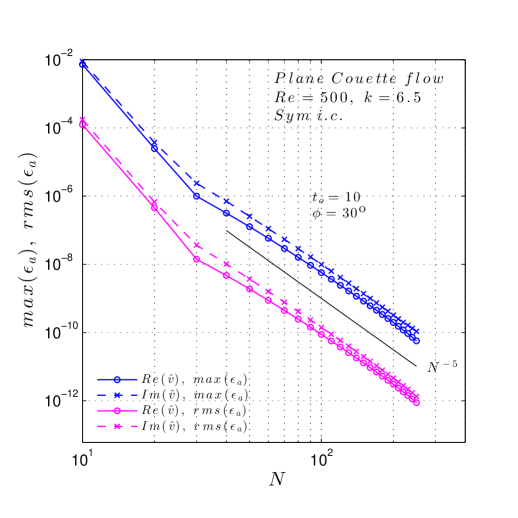
(a) $t_{0}=10$, $Re=500$, $k=6.5$, $\phi=30^{\circ}$

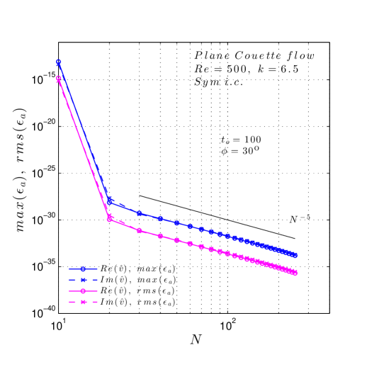
(b) $t_{0}=100$, $Re=500$, $k=6.5$, $\phi=30^{\circ}$

Figure 3.4: Maximum and rms of the absolute residual of $\hat{v}$ for Plane Couette flow and symmetrical (even) initial condition. Continuous line: real part; dashed line: imaginary part. Comparison with $N^{-5}$.

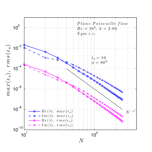
(a) $t_{0}=10$, $Re=1000$, $k=2.04$, $\phi=80^{\circ}$

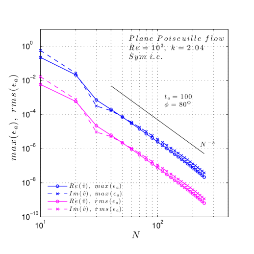
(b) $t_{0}=100$, $Re=1000$, $k=2.04$, $\phi=80^{\circ}$

Figure 3.5: Maximum and rms of the absolute residual of $\hat{v}$ for Plane Poiseuille flow and symmetrical (even) initial condition. Continuous line: real part; dashed line: imaginary part. Comparison with $N^{-5}$.

Convergence of $\hat{\eta}$

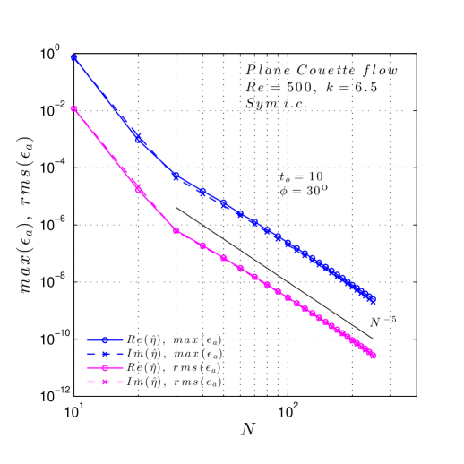
(a) $t_{0}=10$, $Re=500$, $k=6.5$, $\phi=30^{\circ}$

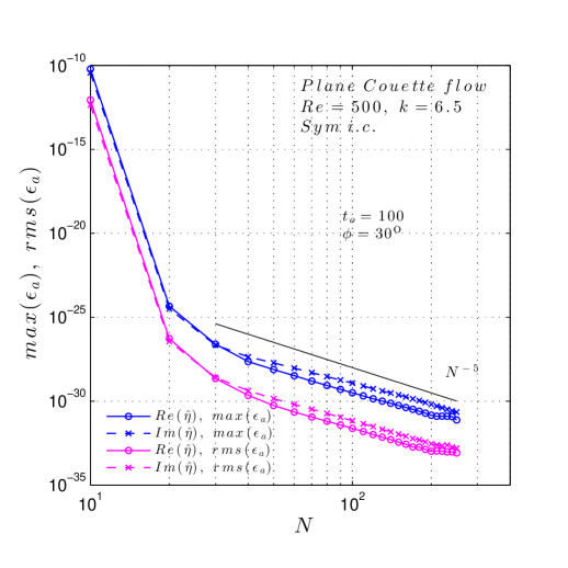
(b) $t_{0}=100$, $Re=500$, $k=6.5$, $\phi=30^{\circ}$

Figure 3.6: Maximum and rms of the absolute residual of $\hat{\eta}$ for Plane Couette flow and symmetrical (even) initial condition. Continuous line: real part; dashed line: imaginary part. Comparison with $N^{-5}$.

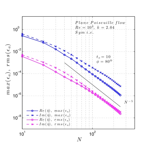
(a) $t_{0}=10$, $Re=1000$, $k=2.04$, $\phi=80^{\circ}$

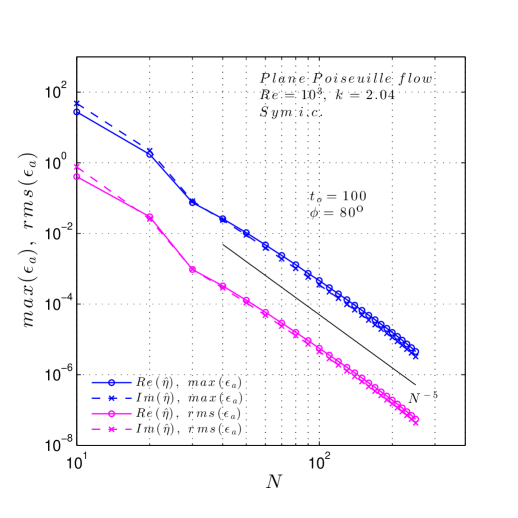
(b) $t_{0}=100$, $Re=1000$, $k=2.04$, $\phi=80^{\circ}$

Figure 3.7: Maximum and rms of the absolute residual of $\hat{\eta}$ for Plane Poiseuille flow and symmetrical (even) initial condition. Continuous line: real part; dashed line: imaginary part. Comparison with $N^{-5}$.

3.4.3   Termwise differentiation and convergence of derivatives

The analytical expressions of the derivatives of the basis functions are known. Thereby, it is easy to investigate the convergence of the series obtained by termwise differentiation. In fact, it is known (see Strauss, 1992) that termwise differentiation is not always possible and if the derivatives of the solution are needed, finite differences techniques may be required. The convergence has been estimated applying the transform to a known function, i.e. the symmetrical initial condition for the normal-velocity. The same profile is used to estimate the convergence for the normal-vorticity, even if it won’t be used as initial condition in the further analysis; thus, in the following figures, the absolute error is indicated as $\epsilon_{a_{ic}}$.
About the convergence of $\hat{v}$, it can be noticed (see Fig. 3.8) that the series can be differentiated termwise three times. The derivative of fourth order converges very slowly in $L_{2}$-norm but the maximum error remains almost constant, which means that the convergence is non-uniform (see Fig. 3.10(a)). The same results have been found by Orszag (1971). The derivatives of lower order converge in both norm to the exact expression, even if the rate decreases with increasing order of derivation. The rate of convergence of $\hat{v}$ is now slightly less than $N^{5}$.

(a) Error $rms$

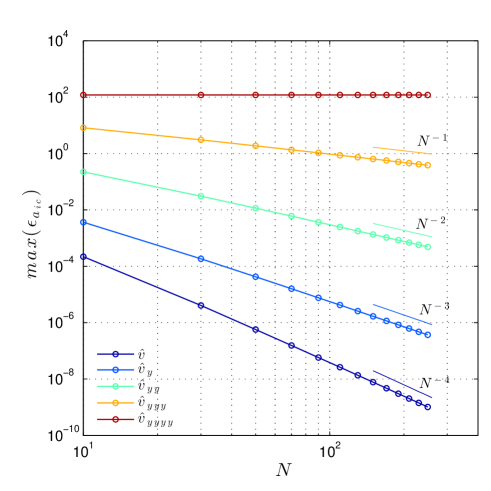
(b) Maximum error

Figure 3.8: Convergence of $\hat{v}$ series and its derivatives to the velocity profile defined by $ic=(1-y^{2})^{2}$.

About $\hat{\eta}$ series, it can be noticed from Fig. 3.9 that the termwise differentiation can be applied to obtain correct results up to the first derivative. The second derivative converges slowly in norm two, but non-uniformly (see Fig. 3.10(b)). In this case the error of $\hat{\eta}$ seems to behave almost like $N^{-3}$, so differently from what can be seen in Fig. 3.6 and Fig. 3.7, where the $\hat{\eta}$ solution is forced by the normal-velocity $\hat{v}$.

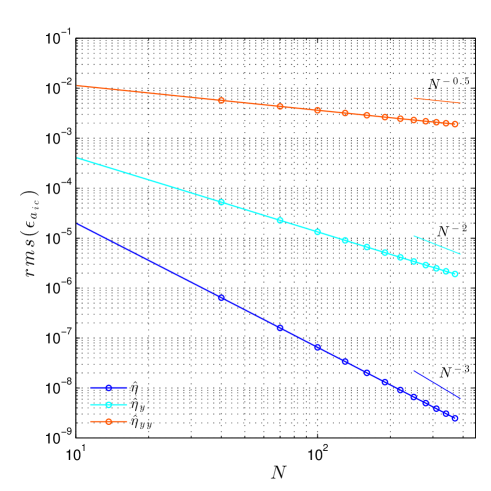
(a) Error $rms$

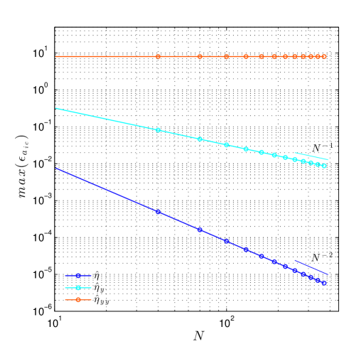
(b) Maximum error

Figure 3.9: Convergence of $\hat{\eta}$ series and its derivatives to a profile defined by $ic=(1-y^{2})^{2}$.

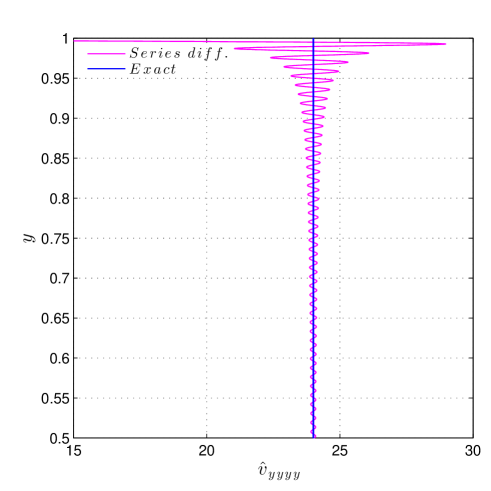
(a)

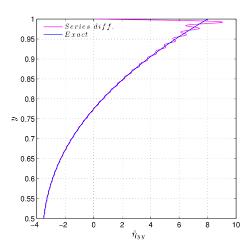
(b)

Figure 3.10: Non-uniform convergence of the four-times termwise differentiated $\hat{v}$ series and of the two-times termwise differentiated $\hat{\eta}$ series to the exact derivatives of $ic=(1-y^{2})^{2}$. The phenomenon is analogous to the Gibbs one, and subsists at the boundaries $y=\pm 1$.

Chapter 4       Wave transient analysis: numerical results

4.1   Introduction

In the present section, particular attention is given to the temporal evolution of the wave frequency and phase velocity. Recent studies (see Scarsoglio et al., 2012, 2009) have been pointing out as through wave frequency investigations precious information can be obtained about the different phases that characterize the spatio-temporal evolution of a perturbation.
The importance of a better understanding of the transient live of traveling waves relies, among other reasons, in the relation with rapid transition to fluid turbulence. In fact, it is believed that the exceptionally large algebraic growth which can occur in the disturbance evolution before the asymptotic exponential mode is set, could promote a phenomenon known as bypass transition (see e.g. Henningson et al., 1994). Actually, it consists of a disturbance growth and breakdown on a timescale much shorter than those typical for Tollmien-Schlichting (TS) waves. The term is used to emphasize that these scenarios bypass the growth of two-dimensional waves and their subsequent secondary instability (see Henningson et al., 1993). It has been shown that the transient algebraic growth can be significant even for subcritical values of the Reynolds number, so that finite amplitudes can rapidly be achieved, and nonlinear effects can enter into play. We will discuss in the next chapter the consequent formation of turbulent spots.

The frequency temporal evolution has been poorly investigated, probably because sheared incompressible flows are viewed as non-dispersive media. Nevertheless, the frequency transient behaviour revealed unexpected phenomena, non predictable a priori, that being related to the wave phase velocity could have a remarkable influence on the main phase speed of a group of waves, in particular on the early stage of a natural spot formation, when the non-linear effects can be neglected, as shown by Cohen et al. (1991) in the case of boundary-layer flow. Moreover, as pointed out by Kachanov (1994), neither intermittence nor turbulent spots are observed in K- or N-regimes of transition when the initial instability wave is strictly periodic in time. The “natural” intermittence phenomena and the spot formation are usually detected when the perturbations background is more complicated and the instability wave has both amplitude and phase modulation in time.

In this contest, the study of the frequency temporal evolution gains more and more importance. From the latest works previously cited emerges that the complexity of the frequency transient is mainly associated to jumps which appear quite far along the temporal history. The normalized time at which the jumps occur have been considered as the threshold between the first two phases of a wave life, respectively the Early transient and the Intermediate transient. The intermediate term lasts until the asymptotic exponential energy growth/decay is reached (long term), and appears to be the most probable state in a wave life, since on one hand its temporal extension is at least one order of magnitude bigger than the early term’s one and, on the other hand, at the end of this intermediate period the disturbance will die or blowup.

In the following sections, an analysis of the phase speed time evolution will be provided; The three phases of a wave life will emerge by taking into account the frequency time history of both the normal-velocity and the normal-vorticity; particularly, the existence of the intermediate period will be shown. Moreover, a relationship between frequency jumps and the achievement of a self-similar asymptotic state of the flow velocity and vorticity profiles will be shown.

4.2   Wave frequency and phase velocity

4.2.1   Analysis of the $\hat{v}$ component of flow velocity

In the present section we take advantage of the solution method proposed in §3.2.2 to obtain the time evolution of the frequency and phase speed of the wall-normal component of velocity $\hat{v}$, varying the three parameters that characterize the problem: the Reynolds number, the obliquity angle and the polar wavenumber. The high non-stationarity of the phenomenon will emerge, typically a jump is observed at a certain time, which is considered to be the threshold between the early period and the intermediate one. After this jump the frequency of $\tilde{v}$ is characterized by a modulation about a constant mean value for Plane Couette flow, for sufficiently high values of the polar wavenumber $k$. For all the simulations performed, $N=250$ eigenfunctions are used for the solution expansion.

Numerical computation

The frequency of the perturbation is defined as the temporal derivative of the unwrapped phase $\theta(y,t;\alpha,\beta)$, at a specific spatial point along the $y$ coordinate. The wrapped phase

$$\theta_{w}(y,t;\alpha,\beta)=arg(\hat{v}(y,t;\alpha,\beta))$$ (4.1)

is a discontinuous function of $t$ in $[-\pi,+\pi]$, while the unwrapped phase $\theta$ is continuous and it is obtained by adding multiples of $\pm 2\pi$ when absolute jumps greater than or equal to $\pi$ radians occur. The wave frequency is defined as

$$\omega(y,t;\alpha,\beta)=\bigg{|}\frac{\partial\theta(y,t;\alpha,\beta)}{\partial t}\bigg{|}$$ (4.2)

The phase velocity vector is given then by the dispersion relation

$$\bm{c}=\frac{\omega}{k}\mathop{}\!\bm{\mathrm{\hat{k}}}$$ (4.3)

where $\mathop{}\!\bm{\mathrm{\hat{k}}}=(cos(\phi),sin(\phi))$ is the unitary vector defining the polar wavenumber direction. The frequency of each signal can be numerically computed at a fixed observation point $y=y_{0}$. In order to ensure a high accuracy in the results, a fourth order centered finite-differences scheme has been used to calculate the first temporal derivative. The following scheme applies for the inner points of the defined time vector and corresponding phase values $(t_{i},\theta_{i})$:

$$\omega(t_{i};y_{0},\alpha,\beta)=\omega_{i}=\frac{\mathrm{d}\theta_{i}}{\mathrm{d}t}=\frac{\theta_{i-2}-8\theta_{i-1}+8\theta_{i+1}-\theta_{i+2}}{12\Delta t}\ \ \ \ i=3,4,\ldots,N_{t}-2$$ (4.4)

where $N_{t}$ is the total number of elements of the time and phase vector and $\Delta t$ the time spacing. It is worth to underline that the proposed method allows the user to define arbitrary time and space grids, differently from Runge-Kutta routines, where the time step is free to change accordingly to the stiffness of the problem and the needed accuracy. This is actually an advantage, because the accuracy of the numerical estimated derivatives is affected by the non-uniformity of the grid. Setting a uniform time spacing we ensure that the finite-differences scheme is actually of the fourth order (see Fertziger & Peric, 1996). Since the scheme stencil is made of five points, for the first and the last two points of the vector respectively a forward and backward fourth order finite-differences scheme is needed. Indeed, the accuracy of the method for these points could be lower. The following schemes are applied:

$$\omega_{1}=\frac{\mathrm{d}\theta_{1}}{\mathrm{d}t}=\frac{-25\theta_{1}+48\theta_{2}-36\theta_{3}+16\theta_{4}-3\theta_{5}}{12\Delta t}$$ (4.5)

$$\omega_{2}=\frac{\mathrm{d}\theta_{2}}{\mathrm{d}t}=\frac{-3\theta_{1}-10\theta_{2}+18\theta_{3}-6\theta_{4}+\theta_{5}}{12\Delta t}$$ (4.6)

$$\omega_{N_{t}-1}=\frac{\mathrm{d}\theta_{N_{t}-1}}{\mathrm{d}t}=\frac{3\theta_{N_{t}}+10\theta_{N_{t}-1}-18\theta_{N_{t}-2}+6\theta_{N_{t}-3}-\theta_{N_{t}-4}}{12\Delta t}$$ (4.7)

$$\omega_{N_{t}}=\frac{\mathrm{d}\theta_{N_{t}}}{\mathrm{d}t}=\frac{+25\theta_{N_{t}}-48\theta_{N_{t}-1}+36\theta_{N_{t}-2}-16\theta_{N_{t}-3}+3\theta_{N_{t}-4}}{12\Delta t}$$ (4.8)

Phase velocity temporal evolution

In the following, the temporal history of the absolute value of the phase velocity of the $\tilde{v}$ component, $|c(t)|$, for the Plane Couette flow is presented, for different combinations of the parameters. As one can be notice from figures 4.1, 4.2, 4.3, 4.4, the problem, though linear, offers a complex highly non-stationary scenario, which is hardly possible to estimate a priori. Two different periods for the phase velocity (and so the frequency) temporal evolution can be observed, the Early term and the Intermediate term. The last one ends when the perturbation energy growth factor reaches the exponential asymptotic trend, and will be investigated in detail in the following section. The transition between the early and the intermediate transient appears to happen in a narrow time window, and it is often characterized by an abrupt jump to a higher mean value which is maintained throughout the rest of the perturbation’s life, indicated as $\bar{c}$ or $\bar{\omega}$ for the phase velocity and the wave frequency respectively.

Another important observation is that the asymptotic value generally is not a constant one for PCf, but a modulation characterized by a specific period $T_{c}$ is present. For this reason it is suitable to refer to frequency asymptotic mean values. A motivation of this fact will be provided in the next paragraph. As it clearly appears from Fig. 4.1(b) and Fig. 4.2(b), the oscillations amplitude can be significant with respect to the mean value, specially for low wavenumbers. With increasing $k$, the frequency temporal evolution appears to shift from peaks-characterized to sinusoidal.

Moreover, it has been verified that exists a certain threshold in the wavenumber, denoted with $k_{j}$, below which neither jump occurs nor phase velocity modulation is observed, but the wave frequency experiences a monotonic decay to the zero value, after a transient evolution (see Fig. 4.1(a), 4.2(a) and Tab. 4.3).
In Tab. 4.1 and Tab. 4.2 values of nondimensional time at which the jump occurs are reported. Since the jump is spread within a certain time window, a strict definition of $T_{j}$ is not provided, so the normalized time corresponding to the frequency peak that typically occurs after the jump is considered, in the present work, as an index of the end of the early transient. Even if the temporal evolution of the wave frequency varies with respect to the simulation parameters and the “jump” itself shows different shapes, some general trends can be observed. In fact, $T_{j}$ seems to increase with increasing Reynolds number (Fig. 4.3(a)) and obliquity angle (Fig. 4.4(a)), while it decreases with increasing polar wavenumber (Fig. 4.3(b)).

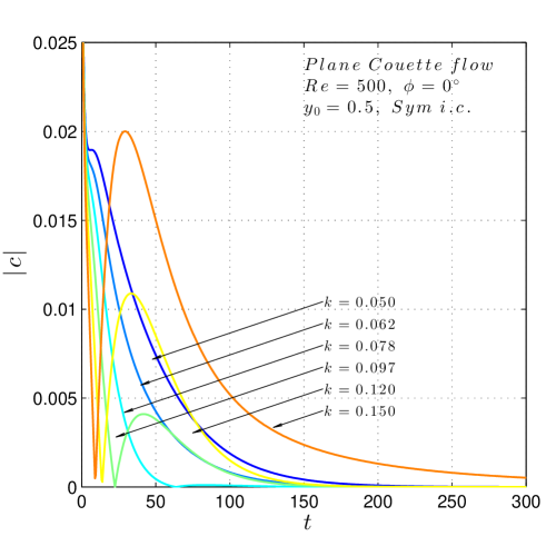
(a)

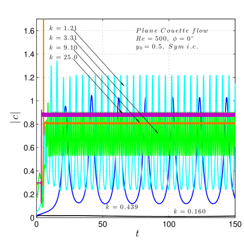
(b)

Figure 4.1: Temporal evolution of the absolute value of the phase velocity, calculated from $\hat{v}$, for PCf at $Re=500$, $\phi=0^{\circ}$ and sym. initial condition, defined by $\hat{v}_{0}=(1-y^{2})^{2}$. The polar wavenumber covers the range $k\in[0.05,25]$, uniformly distributed in the logarithmic space. The fixed observation point is $y_{0}=0.5$.

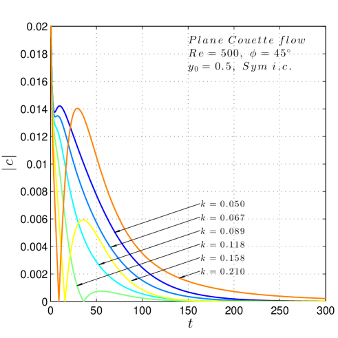
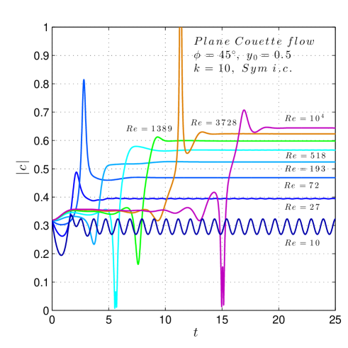
(a)

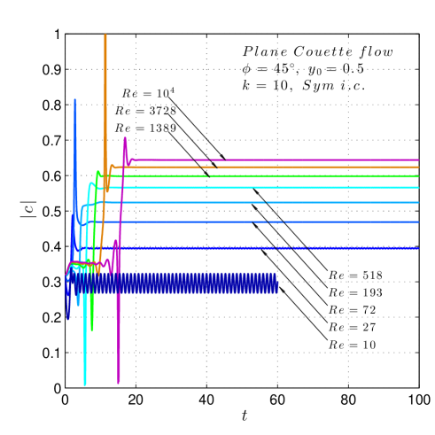
(b)

Figure 4.2: Temporal evolution of the absolute value of the phase velocity, calculated from $\hat{v}$, for PCf at $Re=500$, $\phi=45^{\circ}$ and sym. initial condition. The polar wavenumber covers the range $k\in[0.05,25]$, uniformly distributed in the logarithmic space. The fixed observation point is $y_{0}=0.5$.

(a)

(b)

Figure 4.3: Temporal evolution of the absolute value of the phase velocity, calculated from $\hat{v}$, for PCf for $k=10$, $\phi=45^{\circ}$ and sym. initial condition. The Reynolds number covers the range $Re\in[10,10000]$, uniformly distributed in the logarithmic space. The fixed observation point is $y_{0}=0.5$. (a) Detail of the Early transient and frequency jumps; (b) Intermediate transient.

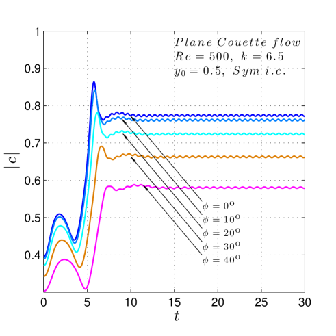
(a)

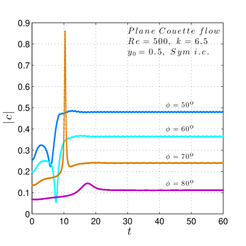
(b)

Figure 4.4: Temporal evolution of the absolute value of the phase velocity, calculated from $\hat{v}$, for PCf for $k=6.5$, $Re=500$ and sym. initial condition. The obliquity perturbation angle covers the range $\phi\in[0^{\circ},90^{\circ}]$, uniformly distributed. The fixed observation point is $y_{0}=0.5$. The case $\phi=90^{\circ}$ is not represented since the orthogonal wave is stationary for all $k$, $Re$ and initial condition.

${k\backslash\phi}$	${0^{\circ}}$	${20^{\circ}}$	${40^{\circ}}$	${60^{\circ}}$	${80^{\circ}}$
$0.80$	10.1	10.9	13.8	23.5	25.0
$1.37$	13.2	14.2	18.1	31.2	96.1
$2.34$	9.00	9.65	12.2	15.3	38.3
$4.00$	5.65	6.02	7.10	10.5	26.2
$6.84$	5.50	5.84	7.15	14.3	16.8
$11.7$	4.47	4.72	5.68	6.75	32.5
$20.0$	3.88	4.14	4.28	7.51	22.5
$34.2$	3.05	3.10	3.90	4.60	15.5
$58.5$	2.15	2.27	2.52	3.40	11.5
$100$	1.41	1.51	1.74	2.32	8.20

Table 4.1: Frequency jump nondimensional time $T_{j}$ for various combination of the simulation parameters, for $Re=500$ and sym. initial condition. $T_{j}$ is considered as the time at which the frequency maximum value, typically located just after the jump, occurs.

${k\backslash\phi}$	${0^{\circ}}$	${20^{\circ}}$	${40^{\circ}}$	${60^{\circ}}$	${80^{\circ}}$
$0.80$	23.8	25.5	31.8	50.7	132
$1.37$	13.6	14.5	18.0	28.2	90.0
$2.34$	8.16	8.72	10.7	16.5	49.4
$4.00$	12.5	13.4	16.5	18.3	56.0
$6.84$	11.6	12.3	15.3	19.2	44.0
$11.7$	10.2	11.0	11.9	16.0	32.4
$20.0$	7.99	8.48	9.56	13.2	26.3
$34.2$	6.47	6.90	7.61	10.5	20.4
$58.5$	4.52	4.62	5.39	7.51	14.5
$100$	3.13	3.33	3.75	5.18	10.1

Table 4.2: Frequency jump nondimensional time $T_{j}$ for various combination of the simulation parameters, for $Re=5000$ and sym. initial condition.

Intermediate Term and Long Term behaviour

An interesting aspect of the nonmodal analysis, hardly ever considered in the past, is the possibility to investigate on how the asymptotic state is reached. In the present and in the following sections some new results will be presented. The trends of the mean values of the asymptotic phase velocity for various combinations of the simulation parameters are reported in Fig. 4.5(a) and Fig. 4.5(b). Accordingly to known results from the cited literature, the phase velocity asymptotic mean value increases with increasing $k$, $Re$ and decreasing $\phi$. The asymptotic value doesn’t depend neither on the initial condition nor on the observation point $y_{0}$, but only on the spectrum of $\hat{v}$ for that particular parameters combination. In fact, the frequency corresponds to the real part of the least damped eigenvalue of the Orr-Sommerfeld operator, while the damping is given by the imaginary part. Even if the present method is developed to study the temporal evolution of perturbations from an initial value problem, the spectra af $\hat{v}$ can easily be obtained by computing the eigenvalues of the matrix $\mathop{}\!\bm{\mathrm{A}}$ (see §3.3.2).
About the mean values of the asymptotic frequency $\bar{\omega}$, trends are shown in Fig. 4.6(a) and Fig. 4.6(b). It can be noticed that for high values of $k$, the general tendency can be approximated by the relation $\bar{\omega}=kcos(\phi)$. This trend was observed for Plane Poiseuile flow and for Wake flow, as well, by Scarsoglio et al. (2012).

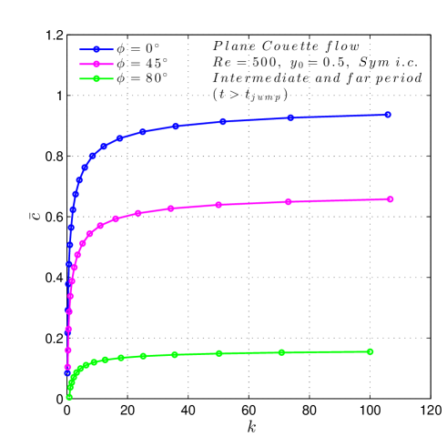
(a)

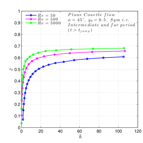
(b)

Figure 4.5: (a) Trends of the absolute mean value of phase velocity, calculated from $\hat{v}$, for PCf for $Re=500$, $\phi=\{0^{\circ},45^{\circ},80^{\circ}\}$ and sym. initial condition. The polar wavenumbers are uniformly distributed in the logarithmic space. The fixed observation point is $y_{0}=0.5$. (b) Absolute mean values of $\bar{c}$, calculated for PCf for $\phi=45^{\circ}$, $Re=\{50,500,5000\}$ and sym. initial condition. These asymptotic results are independent on both the initial condition and $y_{0}$.

(a)

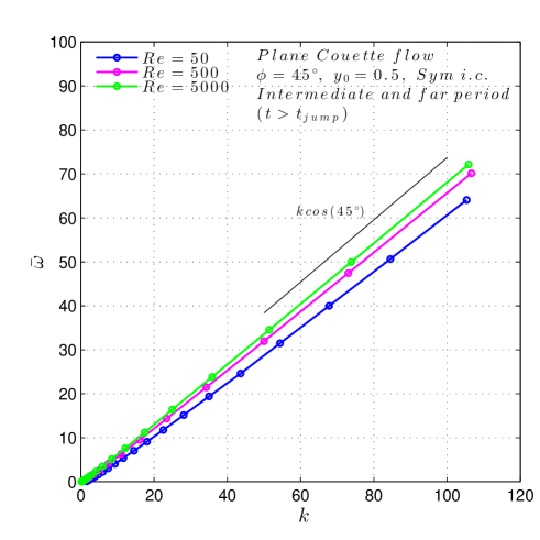
(b)

Figure 4.6: (a) Trends of the absolute mean value of the frequency, calculated from $\hat{v}$, for PCf for $Re=500$, $\phi=\{0^{\circ},45^{\circ},80^{\circ}\}$ and sym. initial condition. The polar wavenumbers are uniformly distributed in the logarithmic space. The fixed observation point is $y_{0}=0.5$. (b) Absolute mean values of $\bar{\omega}$, calculated for PCf for $\phi=45^{\circ}$, $Re=\{50,500,5000\}$ and sym. initial condition. These asymptotic results are independent on both the initial condition and $y_{0}$.

As seen in the previous section, there exists a threshold for $k$ below which the temporal evolution is characterized by a frequency decay to zero, after an early transient. To better observe these conditions, in Fig. 4.7 the phase velocity evolution has been traced on a semilogarithmic plane. Also for these cases there is no influence of the initial condition on the far periods. Moreover it can be noticed that for $k<k_{j}$ there is a phase of exponential decay leading to a stationary state.
The phenomenon has been observed by Gallagher & Mercer (1962) through a modal analysis (2D). They discovered that below a certain value of $\alpha Re$ all the eigenvalues were real. Increasing $Re$, a threshold level is reached, where the least damped eigenvalues are real and coincident; they split into a complex conjugate pair for larger values of the Reynolds number. The authors pointed out the abruptness of the transition, as well. Here various simulations have been performed in order to verify the precision of the method and of the numerical code for the asymptotic solution computation. The results have been compared to those of the cited authors, and an excellent agreement has been found. In addition, a generalization for the three-dimensional case is shown (see Fig. 4.8(b)).
Another comparison have been done with the results obtained by Orszag (1971), who developed a method for the modal analysis based on a Chebyshev polynomials expansion. For Plane Poiseuille flow at $Re=10000,\ \alpha=1$ and $\phi=0^{\circ}$ he found the following value for the unstable eigenvalue: $c=0.23752649+0.00373967i$. With N=250 we obtain the value of $c=0.23752629+0.00373964i$ (with $\Delta y=10^{-3}$, $N=250$). The same accuracy is assured for the the other eigenvalues.

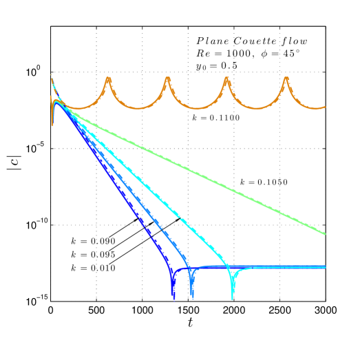
Figure 4.7: Temporal evolution of the absolute value of the phase velocity, calculated from $\hat{v}$, for PCf for $\phi=45$, $Re=1000$. An abrupt variation in the temporal evolution trend can be observed once $k=0.105$ is exceeded. Dot-dashed line: asym initial condition; continuous line: sym i.c.

${Re\backslash\phi}$	${0^{\circ}}$	${45^{\circ}}$	${80^{\circ}}$
$10$	2.9840	3.6900	9.7110
$22$	1.9330	2.3100	5.5150
$46$	1.2850	1.5790	3.4200
$100$	0.7040	0.9420	2.1865
$215$	0.3450	0.4805	1.4610
$464$	0.1620	0.2283	0.8469
$1000$	0.0754	0.1065	0.4239
$2154$	0.0350	0.0495	0.2006
$4642$	0.0162	0.0229	0.0935
$10000$	0.0075	0.0106	0.0434

Table 4.3: Values of threshold wavenumber $k_{j}$ below which the asymptotic frequency tends to zero, i.e the wave tends to a stationary (damped) state at high times. Here $k_{j}$ is reported for three different values of obliquity angle and for ten values of Reynolds number, spanning four decades, uniformly distributed in the logarithmic space.

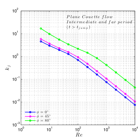
(a)

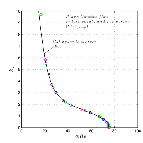
(b)

Figure 4.8: Trends of the threshold wavenumber $k_{j}$ for PCf, as a function of $Re$ for $\phi=\{0^{\circ},45^{\circ},80^{\circ}\}$ (a). Comparison with results found in literature (Gallagher & Mercer, 1962) for the bidimensional case ($\phi=0$). It is worth to notice that here the same trend is found for the three-dimensional cases.

(a)

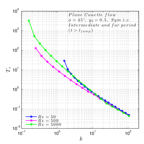
(b)

Figure 4.9: Trends of the phase velocity asymptotic period $T_{c}$ for PCf, as a function of $k$ for $\phi=\{0^{\circ},45^{\circ},80^{\circ}\}$ and $Re=500$ (a). $Re=\{50,500,5000\}$ and $\phi=45^{\circ}$ (b). The observation point $y_{0}$ and the initial condition does not influence the period of the modulation.

We find interesting to investigate the trend and the reasons of the phase velocity asymptotic modulation, since no detailed literature is found about this topic. The modulation is characterized by a period $T_{c}$ that decreases with increasing polar wavenumber, according to an exponential law, for sufficiently high values of $k$ (Fig. 4.9(a)). $T_{c}$ increases with increasing obliquity angle as well, while the influence of $Re$ is weak at high $k$.
Even if further investigations are needed to verify these results, we underline the total agreement with the results obtained by direct numerical integration of (3.1) and (3.2) with the methods of lines and Runge-Kutta ODE solver. In the following we try to provide a motivation about their non-contradictory nature with the modal theory. The spectrum of channel flows (for sufficiently high values of $k$) is generally composed by three branches,whose label $A,P,S$ were given by Mack (1976). In the case of Plane Poiseuille flow all the three branches are present and correspond respectively to wall modes ($c_{r}\to 0$), center modes ($c_{r}\to 1$) and highly damped modes ($c_{r}\to 2/3$). In the case of Plane Couette flow, the spectrum does not contain a $P$ branch but it has two $A$ branches, composed by complex conjugate eigenvalues.

The solution of the initial value problem generally contains the contribute of all the frequency components, as can be clearly seen from the solution of the ODE-reduced velocity equation (3.32). Considering the spectrum of PCf, we observe that there are two least damped, complex conjugate, eigenvalues (with the same damping rate and opposite real frequency). It has been observed, as well, that the coefficients $\mathop{}\!\bm{\mathrm{h_{0}}}$ are complex conjugate; the same does not apply, however, to the final solution where the coefficients are mixed up by the matrix $\mathop{}\!\bm{\mathrm{L}}$ and eventually multiplied by the corresponding shape function $X_{n}$. In this case the phase of the final solution results oscillating and so the frequency. The mean value of the asymptotic frequency corresponds exactly to the real part of the least damped eigenvalues pair.
To support this motivation, simulations have been performed for PPf, for parameters combinations where the least damped eigenvalue is unique. As expected, for these cases no phase velocity oscillations are observed. In the following, some spectra examples for both Plane Couette flow and Plane Poiseuille flow are provided. We remind that in the classical modal analysis the solution, e.g. the normal velocity, is expressed as

$$\hat{v}(y,t)=\hat{\hat{v}}(y)e^{-i\omega t}$$ (4.9)

where $\omega=\omega_{r}+i\omega_{i}$ is the complex eigenvalue, so the real part $\omega_{r}$ represent the wave frequency, while the imaginary component $\omega_{i}$ is damping rate.

According to the convention adopted in the present work (see the exponential terms in (3.32)), the damping rates of the single modes are given by the real part of the eigenvalues, $\mu_{r}=\omega_{i}$ and the frequencies correspond to the imaginary part with changed sign $\mu_{i}=-\omega_{r}$. In order not to be confusing, we will express the spectra with the classical convention found in literature, in terms of phase velocity. Only the least damped eigenvalues are represented in Fig. 4.10 and Fig. 4.11.

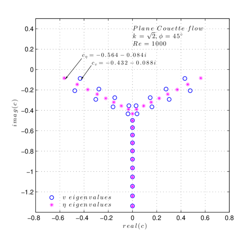
(a)

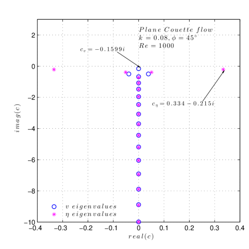
(b)

Figure 4.10: (a) Spectrum of both the Orr-Sommerfeld and the Squire operators for PCf at $Re=1000$, $\phi=45^{\circ}$ and $k=\sqrt{2}$. The least damped eigenvalue, respectively for $\hat{v}$ and for $\hat{\eta}$, is explicitly reported. (b) Spectra for PCf at $Re=1000$, $\phi=45^{\circ}$ and $k=0.08$. Here the polar wavenumber is below the critical value, in fact we observe that the least damped eigenvalue is real. This means that $\hat{v}$ tends to a stationary damped state as $t\to\infty$.

As one can notice, the spectra of the Orr-Somerfeld ($\hat{v}$) and Squire ($\hat{\eta}$) operators are usually different, and for Plane Couette flow in many cases the least damped eigenvalue belong to the set of the Squire operator (see for example Fig. 4.10(a)). this fact is found to have an influence on the dynamic of the system which has not been taken in account yet, as shown in the next section.

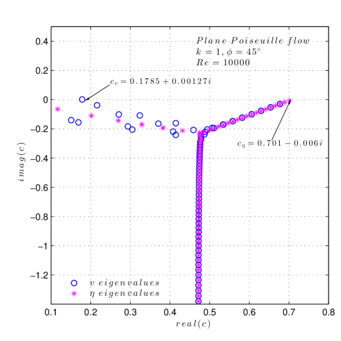
(a)

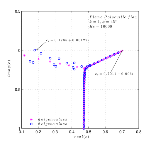
(b)

Figure 4.11: (a) Spectrum of both the Orr-Sommerfeld and the Squire operators for PPf at $Re=1000$, $\phi=45^{\circ}$ and $k=1$. This is an instable configuration: an eigenvalue with positive imaginary part exists. (b) Spectra for PCf at $Re=1000$, $\phi=45^{\circ}$ and $k=10$. With increasing $k$, or $Re$, the eigenvalues exact computation becomes difficult. The issue concerns the sensitivity of the spectrum to small perturbations (e.g. the computer finite precision). This is a property of the linear operator rather than a property of the numerical scheme, and the junction point of the three branches exhibit the largest sensitivity (see Schmid & Henningson, 2001). However, the validity of the solution is not compromised, since the problem doesn’t affect the first eigenvalues.

4.2.2   Behaviour of the vorticity component $\hat{\eta}$ and global considerations

In order to understand the behavior of the complete solution, the normal vorticity must be considered or, alternatively, the other components of perturbation velocity $\hat{u}$ and $\hat{w}$. In the present section the phase velocity of the vorticity signal is investigated and some new results are presented. The same fourth order finite-difference scheme introduced in §4.2.1 is used for the computation of the phase first derivative.

Temporal evolution of the $\hat{\eta}$ phase velocity

As seen in the previous section, the non-modal analysis allows to observe the complete life of a perturbation, from the early transient to the asymptotic state predicted by the modal analysis. However, in the past the same frequency for both the normal velocity and the normal vorticity (or, similarly, for the three components of velocity) was usually considered by the authors dedicated to the modal analysis. As pointed out by Schmid & Henningson (2001), only the particular solution of the modal Squire equation has the same frequency of $\tilde{v}$. In the following analysis, the role of the homogeneous part $\hat{\eta}_{h}$ in the frequency temporal evolution of $\tilde{\eta}$ is shown. Moreover in the following section we will focus on the evolution of the velocity and vorticity profiles along the $y$ coordinate, and their correlation with the frequency time history.

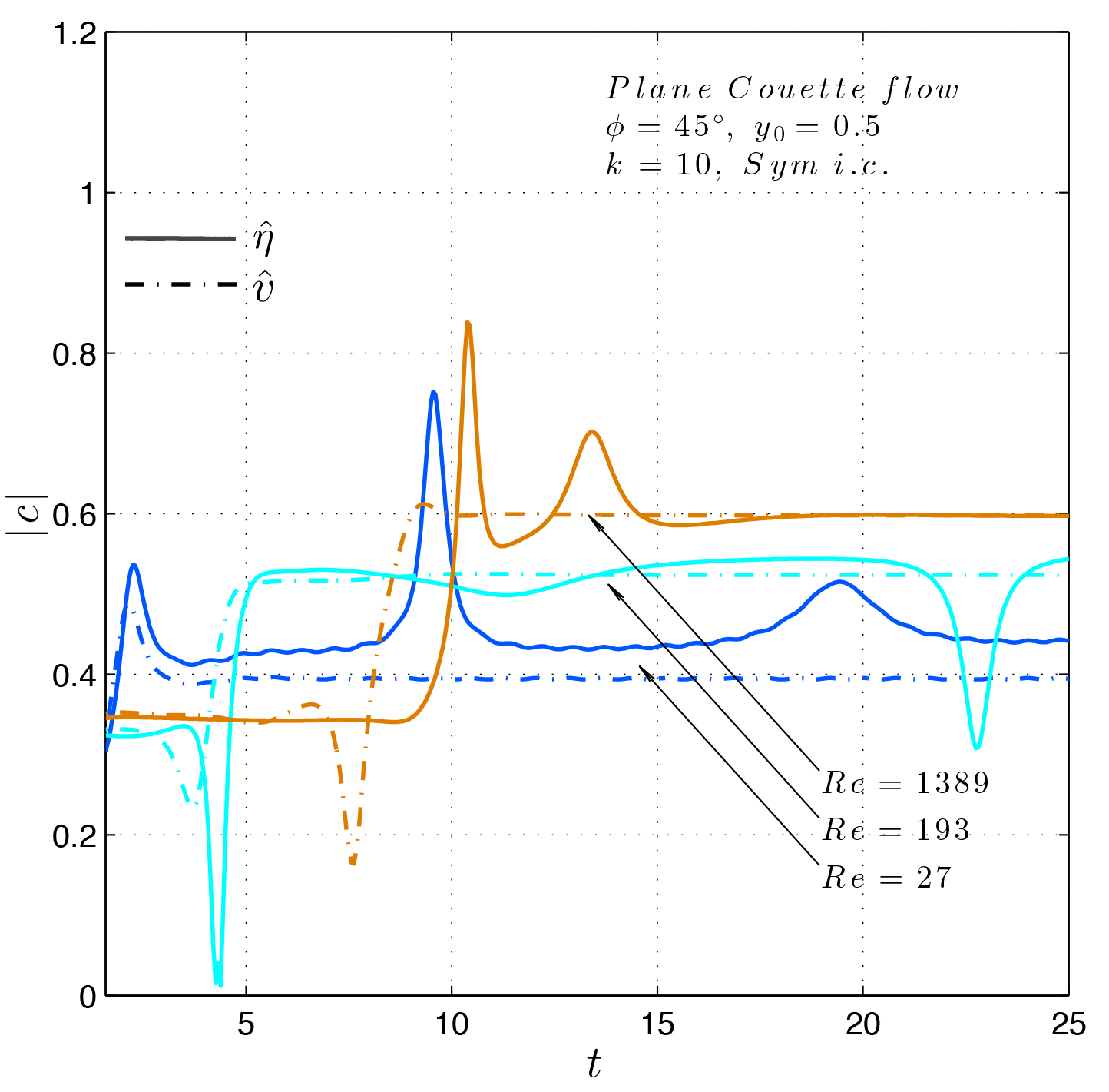
(a)

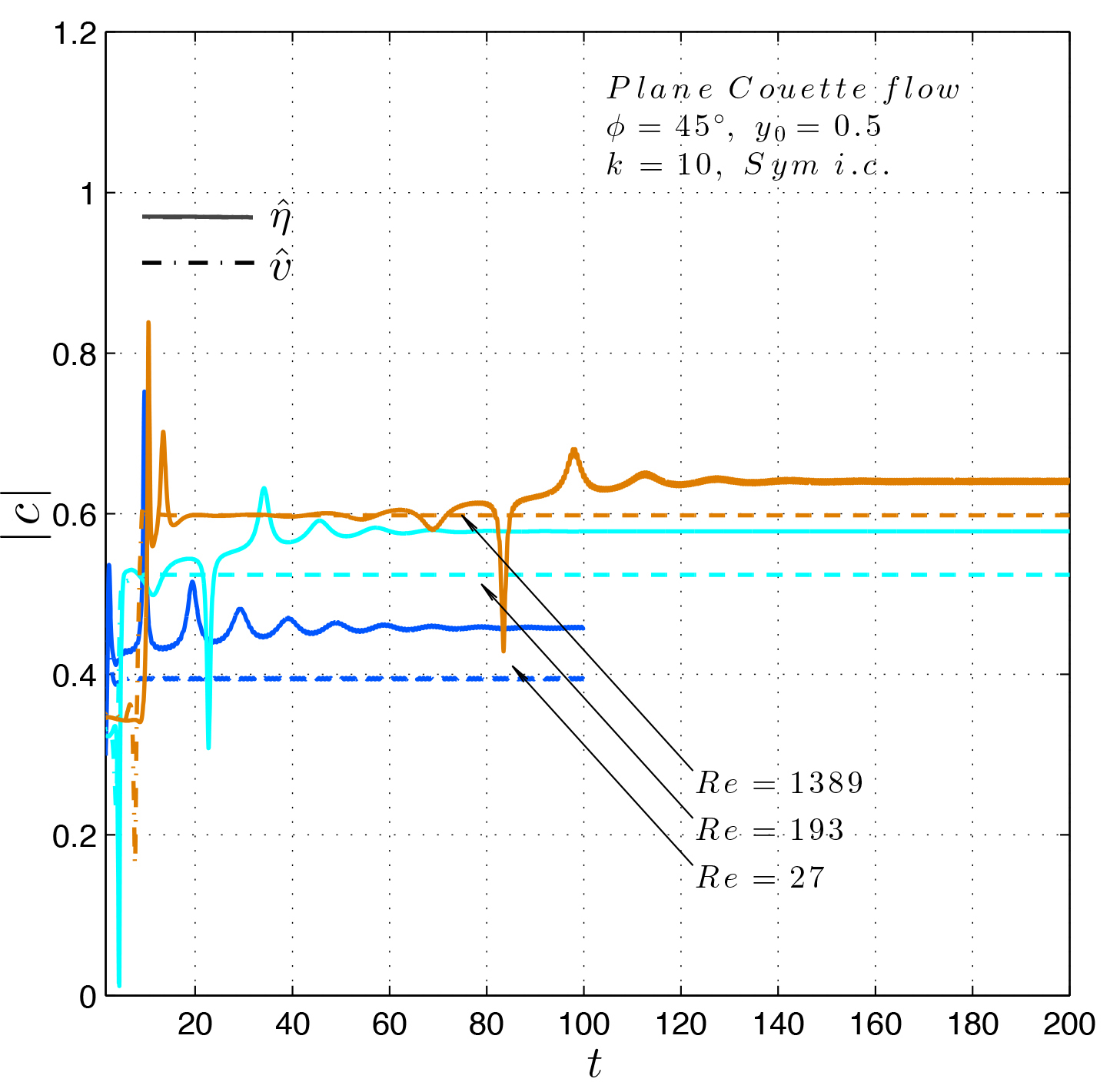
(b)

Figure 4.12: Temporal evolution of the absolute value of the phase velocity, calculated from $\hat{\eta}$ (continuous line), for PCf for $k=10$, $\phi=45^{\circ}$, $Re=\{27,193,1389\}$ and sym. initial condition.The fixed observation point is $y_{0}=0.5$. (a) Detail of the early transient and first frequency jump; (b) Intermediate and far transient: the second jump can be observed. The phase velocity of $\tilde{v}$ is shown with dot-dashed lines.

As shown in Fig. 4.12(a), for sufficiently high values of $Re$, the phase velocity of $\tilde{\eta}$ ($c_{\eta}$, in the following) has approximately the same evolution of the phase velocity of $\tilde{v}$ analized in the previous section, $c_{v}$ in the following, even if it is clear that they are not coincident. To be more precise, a certain lag in the first jump time $T_{j}$ is observed.
Figure 4.12(b) reveals an interesting aspect: the frequency of $\tilde{\eta}$ experiences a second jump, after which it reaches the asymptote predicted by the modal theory. In the time window between the these two jumps the mean value of $c_{\eta}$ is about the one of $c_{v}$, and this phase of the wave life can also last several time units, depending on the parameters. In fact, the time at which the second jump, $T_{j2}$, occurs increases with increasing $Re$ and with decreasing $k$, while about the influence of the obliquity angle, we observe that $T_{j2}$ increases with increasing $\phi$ for high $k$, but the opposite trend occurs at lower wavenumbers (see Tab. 4.4).

${k\backslash\phi}$	${20^{\circ}}$	${40^{\circ}}$	${60^{\circ}}$	${80^{\circ}}$
$0.80$	1030	860	710	475
$1.37$	420	352	334	332
$2.34$	176	164	170	194
$4.00$	96.2	97.0	112	162
$6.84$	45.5	53.5	58.0	94.0
$11.7$	38.8	46.0	50.8	85.4
$20.0$	34.8	41.5	45.5	79.0
$34.2$	23.9	37.6	42.2	75.3

Table 4.4: Frequency jump nondimensional time $T_{j2}$ for various combination of the simulation parameters, for $Re=500$ and sym. initial condition. Since the transition to the asymptotic value of $c_{\eta}$ can be more or less smooth, $T_{j2}$ is considered as the time at which the frequency peak, typically located just after the jump, occurs.

Intermediate Term and Long Term behaviour

In order to understand the physical reasons why $c_{\eta}$ experiences two jumps during its temporal evolution, we take advantage of the mathematical formulation introduced in §3.2 and §3.3. The Squire equation (3.2) is forced by the solution $\hat{v}$ of the Orr-Sommerfeld PDE (3.1). The general solution can be expressed as $\hat{\eta}=\hat{\eta}_{h}+\hat{\eta}_{p}$ as shown in §3.3.2. The particular solution contains the same eigenvalues spectrum of the forcing $\hat{v}$, while the spectrum of the Squire operator (the homogeneous part) $\hat{\eta}_{h}$ is different. Thinking about a generic forced linear system, it is clear that the asymptotic solution has the same frequency of the forcing term if its amplitude is constant. If the forcing term itself is damped, the asymptotic frequency depends on the damping of both the forcing term and the homogeneous solution. If the damping rate of the forcing term is higher than the one of the homogeneous operator, the frequency for $t\to\infty$ will be the “natural pulsation” of the system.
Here the system is far more complicated but the same phenomenon is observed; for several configurations of the parameters, looking at the spectra (e.g. Fig. 4.10, Fig. 4.11) one can notice that the least damped eigenvalue belongs to the Squire set. In these cases, the second jump of $c_{\eta}$ occurs. $T_{j2}$ depends on the initial coefficients of the series $\mathop{}\!\bm{\mathrm{h_{0}}}$ (i.e. on the initial condition) and on the ratio of the real part of the eigenvalues $\mu$, to $\mu^{*}$, and can be qualitatively considered as the end of the intermediate term and the beginning of the asymptote, as can be seen from the trends of the kinetic energy growth rate in Fig. 4.13.

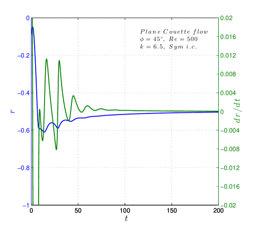
(a)

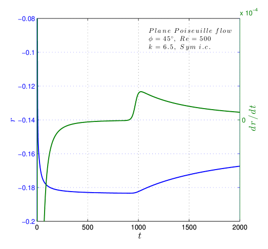
(b)

Figure 4.13: Temporal evolution of the kinetic energy growth rate (blue line ) and its derivative (green line) for PCf with $k=6.5$, $\phi=45^{\circ}$, $Re=500$ and sym. initial condition. It is evident a correlation with the frequency jumps shown in the following plots.

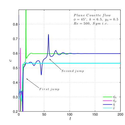
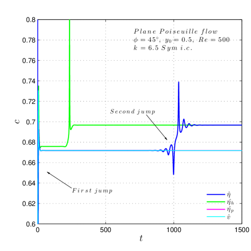
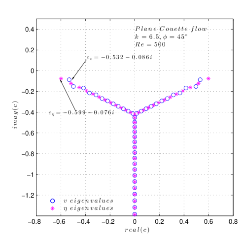
(a)

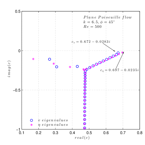
(b)

Figure 4.14: (a) Temporal evolution of the absolute value of the phase velocity of $\tilde{\eta}$, $\tilde{\eta}_{h}$, $\tilde{\eta}_{p}$ and comparison with $c_{v}$ for PCf with $k=6.5$, $\phi=45^{\circ}$, $Re=500$ and sym. initial condition (upper plot). In the lower plot the spectrum for the same configuration is shown. (b) Phase velocity for Plane Poiseuille flow, same parameters configuration. In both cases the least damped eigenvalue belongs to the Squire set.

For Plane Couette flow, the same modulation observed in the phase velocity of $\tilde{v}$ is found in the $\tilde{\eta}$ component, even if the characteristic amplitude and the period are generally different. The same motivation discussed in the previous section applies, the eigenvalues of $\hat{\eta}$ for this type of flow are complex conjugate, indeed. The frequency of this modulation appears to be generally higher than the one of $c_{v}$ , supporting the fact that this modulation is related to the imaginary part of the least damped $\mu_{i}$ (for $c_{v}$) or $\mu^{*}_{i}$ (for $c_{\eta}$), as can be inferred by looking at the spectra, since usually $|\Re(c_{v})|<|\Re(c_{\eta})|$ for the least damped. The trend of the asymptotic frequency is reported in Fig. 4.15(a) and Fig. 4.15(b), where one can see that as $k\to\infty$ the difference between $c_{v}$ and $c_{\eta}$ tends to vanish. Anyway the general trend of the two frequencies, varying the parameters, is approximately the same.

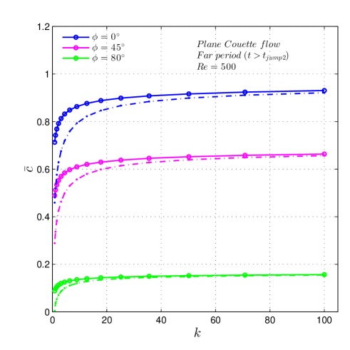
(a)

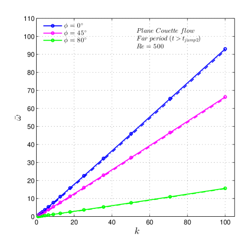
(b)

Figure 4.15: (a) Asymptotic absolute values of $c_{\eta}$, for PCf with $Re=500$, $\phi=\{10^{\circ},45^{\circ},80^{\circ}\}$. The polar wavenumbers are uniformly distributed in the logarithmic space. (b) Asymptotic absolute values of ${\omega_{\eta}}$. Comparison with the trends of $\bar{c}_{v},\ \bar{\omega}_{v}$, plotted with dot-dashed line.

4.3   Velocity and vorticity profiles, similarity considerations and solutions in the physical space

4.3.1   Profiles of $\hat{v}$, $\hat{\eta}$ and their similarity properties

In this section, the temporal evolution of the normal vorticity and velocity profiles along the $y$ coordinate is investigated. We observe that the frequency jumps previously introduced are strictly related to the spatial distribution of the solutions $\hat{v}$ and $\hat{\eta}$, i.e. to the distribution of the complete flow field, in the wavenumber space. In figures 4.16-4.22 the velocity and vorticity profiles are reported, together with the phase velocity time history and the evolution of the first derivative of the kinetic energy growth rate. Actually, the quantities analyzed in the following are the modules of the complex-valued solutions $\hat{v}$ and $\hat{\eta}$

$$|\hat{v}|=\sqrt{\Re^{2}{\hat{v}}+\Im^{2}{\hat{v}}}\hskip 42.67912pt|\hat{\eta}|=\sqrt{\Re^{2}{\hat{\eta}}+\Im^{2}{\hat{\eta}}}$$ (4.10)

The module of the general quantity in the wavenumber space can be related to the solution in the physical space. In fact, taking advantage of linearity, the inverse transform for a single wave reads (Criminale, 2003)

$$\tilde{v}(x,y,z,t)=\frac{1}{2}\left[\hat{v}(y,t)e^{i\alpha x+i\beta z}+\hat{v}^{*}(y,t)e^{-i\alpha x-i\beta z}\right]$$ (4.11)

$$\tilde{\eta}(x,y,z,t)=\frac{1}{2}\left[\hat{\eta}(y,t)e^{i\alpha x+i\beta z}+\hat{\eta}^{*}(y,t)e^{-i\alpha x-i\beta z}\right]$$ (4.12)

where the * sign represents the complex conjugate. Hence, the sum of the first complex quantity at right hand side and its conjugate represents the real disturbance quantity in the physical space; the same applies for $\tilde{u}$ and $\tilde{w}$, derived from (2.25) and (2.26). Since the complex conjugate values can be easily obtained once $\hat{v}$ and $\hat{\eta}$ are computed, this is a convenient way to express the solution.
The explicit relation between the real and imaginary part of the solutions and the quantities in the physical space is derived from the above expressions

$$\tilde{v}(x,y,z,t)=\Re\hat{v}\ cos(\alpha x+\beta z)-\Im\hat{v}\ sin(\alpha x+\beta z)$$ (4.13)

$$\tilde{\eta}(x,y,z,t)=\Re\hat{\eta}\ cos(\alpha x+\beta z)-\Im\hat{\eta}\ sin(\alpha x+\beta z)$$ (4.14)

The profile along the coordinate $y$ of the module $|\hat{v}|(y,t)$ or $|\hat{\eta}|(y,t)$ indicates the envelope of the maxima of $\tilde{v}$, or $\tilde{\eta}$, at a fixed point $(x,z)$

$$|\hat{v}|(y,t_{0})=\max_{x,z}\{\tilde{v}(x,y,z,t_{0})\}$$ (4.15)

$$|\hat{\eta}|(y,t_{0})=\max_{x,z}\{\tilde{\eta}(x,y,z,t_{0})\}$$ (4.16)

The following figures show how the temporal evolution of the disturbance phase velocity is closely related to the spatial distribution. To be more precise, the solution in terms of modules seems to achieve a self-similarity in time, when the frequency becomes constant. In fact, in these conditions the profiles coincide if normalized with their $L_{\infty}$-norm (the maximum along $y$) or, similarly, with the $L_{2}$-norm. This means that the space-dependent and time-dependent parts of the solution are separable.

$$\frac{|\hat{v}|(y,t)}{(\max_{y}\hat{v})(t)}=f(y)\hskip 42.67912ptSelf-similarity$$ (4.17)

Usually the component of normal velocity is found to achieve this condition after $T_{j}$, the time at which the first frequency jump occurs, as shown in Fig. 4.16-4.17 for Plane Couette flow, and Fig. 4.18-4.21 for Plane Poiseuille flow. The vorticity profile continues to evolve until the second phase velocity transition occurs, for $t=T_{j2}$. For the cited cases, we observe that for PCf the $|\hat{\eta}|$ spatial distribution varies quite smoothly (Fig. 4.17) while for PPf an abrupt variation in the parity of the profile occurs (the double hump of the modules correspond to odd profiles in the physical plane), as shown in Fig. 4.19.

An interesting case is shown in Fig. 4.20-4.21, where the sudden profile change, and the associated second frequency jump are experienced by the velocity component rather than the vorticity one. This is probably due to the influence of the antisymmetrical initial condition on the early and intermediate wave transient. This influence may be related to the parity of the asymptotic state, which is independent on the initial condition. It is also interesting to notice that the intermediate phase, starting after the first jump, is usually very close to similarity conditions; in this term, the phase velocities of the two signals are nearly coincident. Moreover, we underline that the intermediate transient is, in addition to the early period, the most relevant term in a perturbation’s life. Indeed, in the introduced cases $T_{j2}$ occurs when the wave kinetic energy is extremely small (the last jump represents the beginning of the asymptotic conditions).

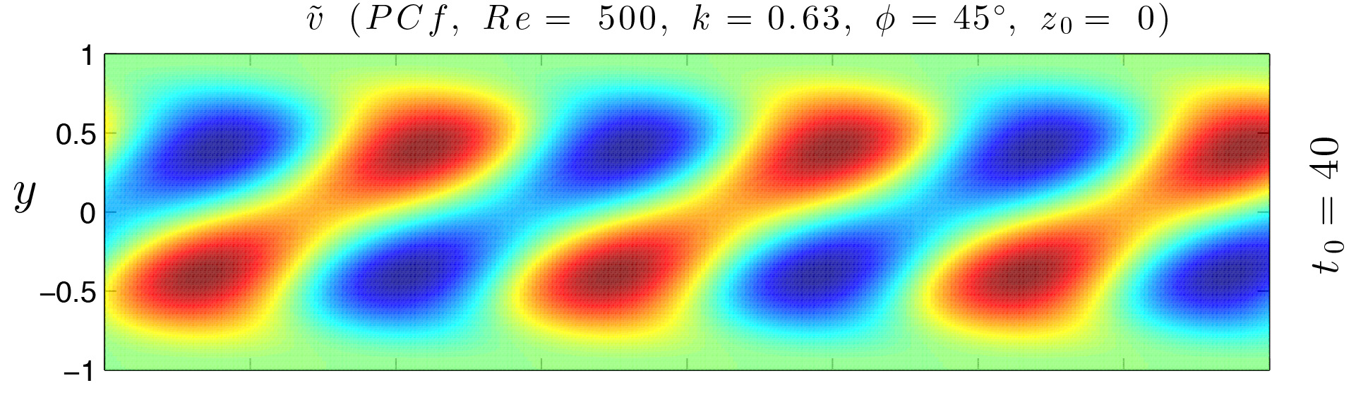
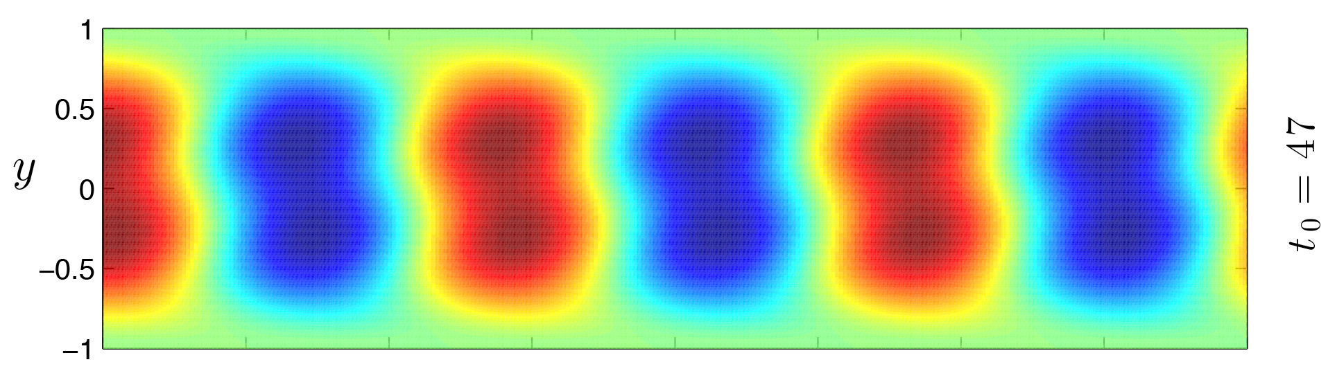
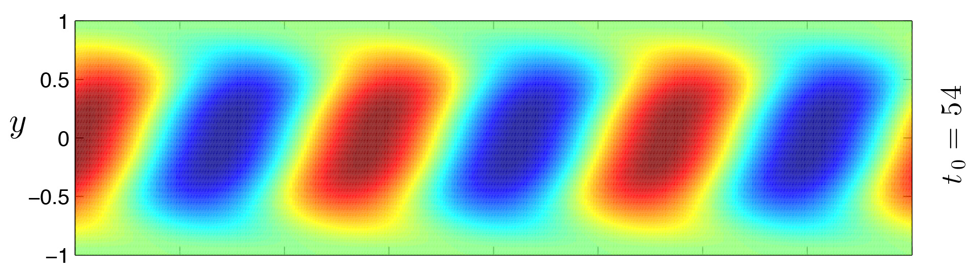
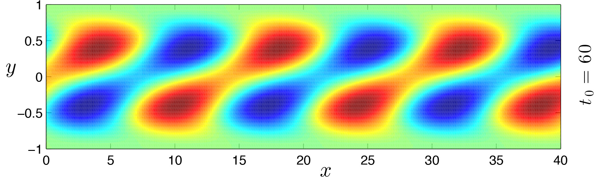
Figure 4.30: Visualization of the wall-normal perturbation velocity $\tilde{v}(x,y,z_{0},t_{0})$, $xy$ plane, for Plane Couette flow. This low-wavenumber condition was introduced and analyzed in Fig. 4.22. From the physical space, the high non-stationarity of the whole scenario is evident. The two opposite moving layers, where the largest disturbances reside, appears to experience a periodic attachment and consecutive detachment. The images sequence represents one period in the modulation of $c_{v}$, the maximum of phase velocity occurs in the conditions (a) and (d). Red: maximum (positive); blue: minimum (negative).

A connection between the periodic frequency modulation observed for Plane Couette flow in §4.2.1 and the spatial distribution is pointed out in Fig. 4.22; here it should be noticed that a periodic continuous variation in the (normalized) profiles of $|\hat{v}|$ and $|\hat{\eta}|$ occurs. Actually, the periodic change happens in the channel central region, while the near-wall region remains unchanged and self-similar. The corresponding case in the physical space is reported in Fig. 4.30.

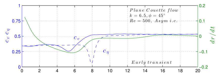
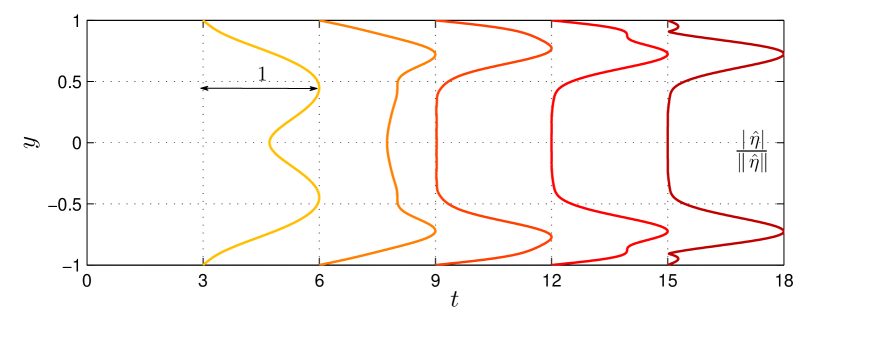
Figure 4.16: Plane Couette flow early transient for $Re=500$, $\phi=45^{\circ}$, $k=6.5$ and asym. initial condition. Top: phase velocity temporal evolution for the $\hat{v}$ and $\hat{\eta}$ disturbance (respectively, blue continuous line and blue dashed line) and first derivative of the kinetic energy growth rate (green line). Middle: profiles of the modulus of $\hat{v}$, normalized with respect to the maximum ($L_{\infty}$-norm). Bottom: profiles of $|\hat{\eta}|/\|\hat{\eta}\|_{\infty}$.

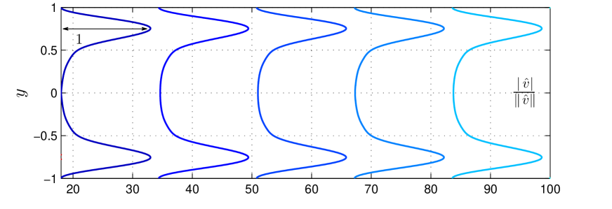
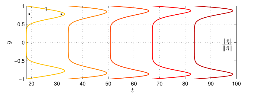
Figure 4.17: Plane Couette flow intermediate and far term for $Re=500$, $\phi=45^{\circ}$, $k=6.5$ and asym. initial condition. Top: phase velocity temporal evolution for the $\hat{v}$ and $\hat{\eta}$ disturbance (respectively, blue continuous line and blue dashed line) and first derivative of the kinetic energy growth rate (green line). Middle: profiles of the modulus of $\hat{v}$, normalized with respect to the maximum ($L_{\infty}$-norm). Bottom: profiles of $|\hat{\eta}|/\|\hat{\eta}\|_{\infty}$. Note that $|\hat{v}|$ is fully self-similar after the first jump, while $|\hat{\eta}|$ achieves gradually the similarity after the second jump.

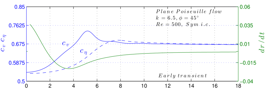
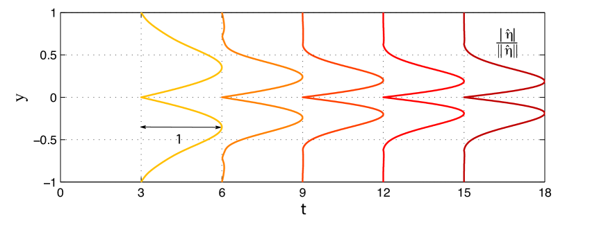
Figure 4.18: Plane Poiseuille flow early transient for $Re=500$, $\phi=45^{\circ}$, $k=6.5$ and sym. initial condition. Top: phase velocity temporal evolution for the $\hat{v}$ and $\hat{\eta}$ disturbance (respectively, blue continuous line and blue dashed line) and first derivative of the kinetic energy growth rate (green line). Middle: profiles of the modulus of $\hat{v}$, normalized with respect to the maximum ($L_{\infty}$-norm). Bottom: profiles of $|\hat{\eta}|/\|\hat{\eta}\|_{\infty}$.

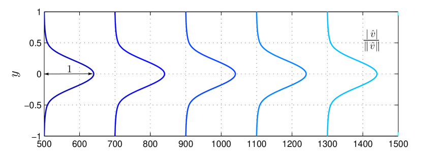
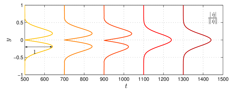
Figure 4.19: Plane Poiseuille flow intermediate and far term for $Re=500$, $\phi=45^{\circ}$, $k=6.5$ and sym. initial condition. Top: phase velocity temporal evolution for the $\hat{v}$ and $\hat{\eta}$ disturbance (respectively, blue continuous line and blue dashed line) and first derivative of the kinetic energy growth rate (green line). Middle: profiles of the modulus of $\hat{v}$, normalized with respect to the maximum ($L_{\infty}$-norm). Bottom: profiles of $|\hat{\eta}|/\|\hat{\eta}\|_{\infty}$. It is interesting to notice the abrupt transition to the final state of the vorticity profile, which occurs in correspondence to the second frequency jump. Both the states before and after $T_{j2}$ seem to have similarity properties.

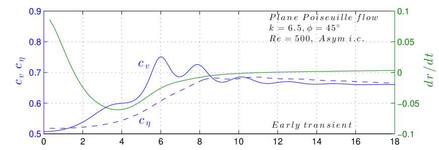
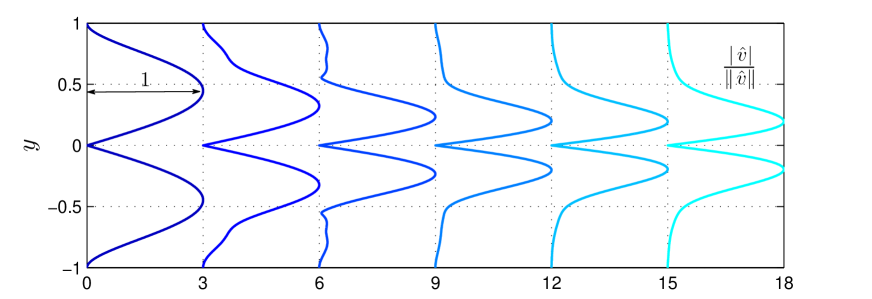
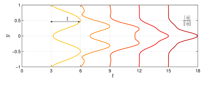
6

Figure 4.20: Plane Poiseuille flow early transient, for $Re=500$, $\phi=45^{\circ}$, $k=6.5$ and asym. initial condition. Top: phase velocity temporal evolution for the $\hat{v}$ and $\hat{\eta}$ disturbance (respectively, blue continuous line and blue dashed line) and first derivative of the kinetic energy growth rate (green line). Middle: profiles of the modulus of $\hat{v}$, normalized with respect to the maximum ($L_{\infty}$-norm). Bottom: profiles of $|\hat{\eta}|/\|\hat{\eta}\|_{\infty}$.

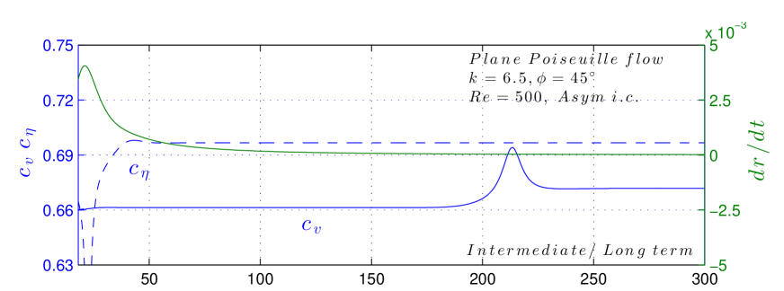
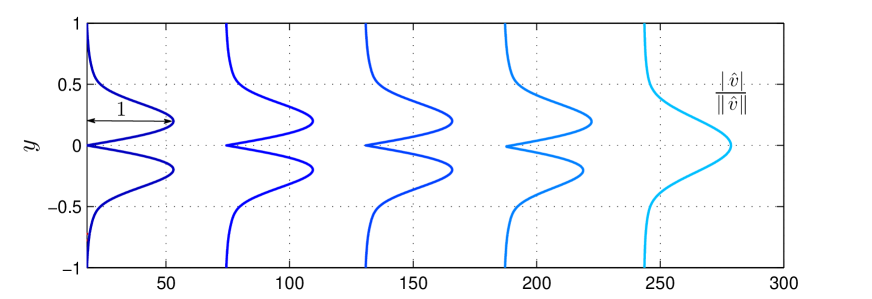
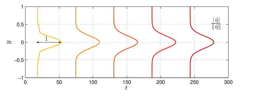
Figure 4.21: Plane Poiseuille flow intermediate and far term for $Re=500$, $\phi=45^{\circ}$, $k=6.5$ and asym. initial condition. Top: phase velocity temporal evolution for the $\hat{v}$ and $\hat{\eta}$ disturbance (respectively, blue continuous line and blue dashed line) and first derivative of the kinetic energy growth rate (green line). Middle: profiles of the modulus of $\hat{v}$, normalized with respect to the maximum ($L_{\infty}$-norm). Bottom: profiles of $|\hat{\eta}|/\|\hat{\eta}\|_{\infty}$. The difference from the case of $Fig.\leavevmode\nobreak\ \ref{fig:prof_PO_Re500_k6p5_far_sym}$ should be noticed: indeed, here $|\hat{v}|$ stabilizes to the final self-similar state after the vorticity component. This state is announced by a the second transition of $c_{v}$ rather than the “usual” one of $c_{\eta}$. This is likely due to the combination of the symmetry properties of both the initial condition (here antisymmetrical) and the asymptotic states.

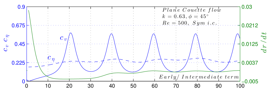
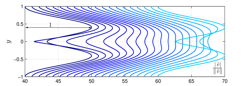
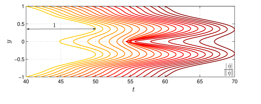
Figure 4.22: Plane Couette flow intermediate and far term for $Re=500$, $\phi=45^{\circ}$, $k=0.63$ and sym. initial condition. Top: phase velocity temporal evolution for the $\hat{v}$ and $\hat{\eta}$ disturbance (respectively, blue continuous line and blue dashed line) and first derivative of the kinetic energy growth rate (green line). Middle: profiles of the modulus of $\hat{v}$, normalized with respect to the maximum ($L_{\infty}$-norm). Bottom: profiles of $|\hat{\eta}|/\|\hat{\eta}\|_{\infty}$. This is an interesting case characterized by large frequency oscillations; the modulation of phase velocity is related to a periodic variation of the normalized profiles of both $|\hat{v}|$ and $|\hat{\eta}|$.

4.3.2   Maxima of kinetic energy for Plane Couette flow

Even if the focus of the chapter is on the wave frequency and the similarity properties of the velocity profiles, it is thought to be appropriate to include this little paragraph about the maxima gained by the kinetic energy during the perturbation’s life. The maps of figures 4.23-4.26, together with the evolution of the real normalized velocity and vorticity fields introduced in the next paragraph, contribute to gain understanding of the complete scenario.

It is known that in the early and intermediate terms even large transient growths can be experienced by the components of flow velocity, vorticity, and by the kinetic energy. The normalized kinetic energy density $G$ defined in §2.1.3 can effectively measure the transient growth for a perturbation with prescribed initial condition. Following the definition by Criminale (2003), an asymptotically stable configuration is called algebraically unstable if $G>0$ for some $t>0$; algebraically stable if $G<0$ for all time; algebraically neutral if $G=0$ for all time. The reasons for the algebraic growth are mainly three. First, the non-orthogonality of the eigenfunctions, as shown by Schmid & Henningson (2001). Secondly, a possible resonance between the Orr-Sommerfeld and the Squire damped exponential modes can occur, as shown by Benney & Gustavsson (1981). However, the resonance does not occur for the boundary layer. The last reason deals with the presence of a continuous spectrum (so, it only applies to unbounded flows), see the work by Criminale & Drazin (1990).

In the following, the maxima of $G$ are traced as a function of the obliquity angle. The nondimensional time at which the maxima occurs is reported as well. Curves for six values of Reynolds number (Fig. 4.23 and Fig. 4.25) and polar wavenumber (Fig. 4.24 and Fig. 4.26) are shown, for both the symmetrical (Fig. 4.23 and Fig. 4.24) and the antisymmetrical initial condition (Fig. 4.25 and Fig. 4.26). It is interesting to notice that, for fixed $Re$ and $k$ , it is not generally true that the maximum occurs for $\phi=90^{\circ}$. This is evident from Fig. 4.26.

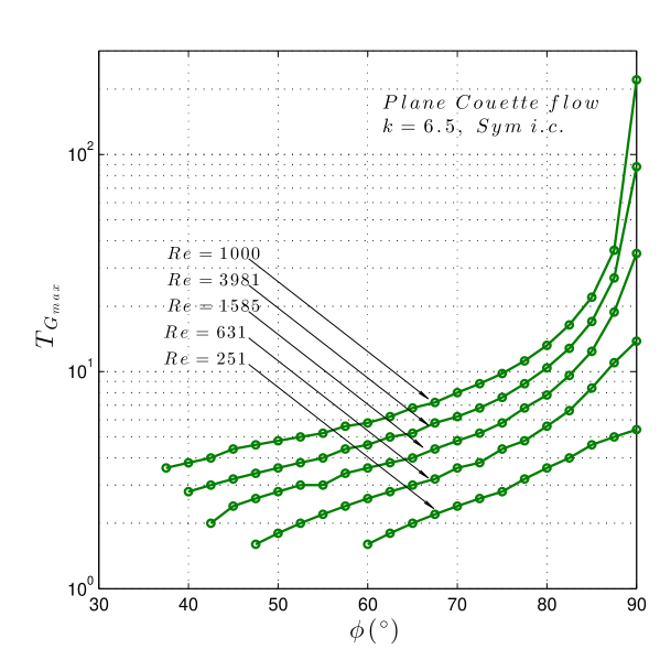
Figure 4.23: Upper plot: maxima of the kinetic energy density $G$ as a function of the obliquity angle $\phi$, parametrized with $Re$, for Plane Couette flow with $k=6.5$ and antisymmetrical initial condition. Lower plot: nondimensional times corresponding the the maxima of $G$. The values of Reynolds number are uniformly distributed in the logarithmic space.

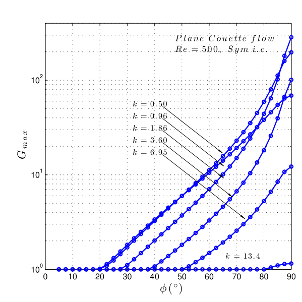
Figure 4.24: Upper plot: maxima of the kinetic energy density $G$ as a function of the obliquity angle $\phi$, parmetrized with $k$, for Plane Couette flow with $Re=500$ and symmetrical initial condition. Lower plot: nondimensional times corresponding the the maxima of $G$. The values of polar wavenumber are uniformly distributed in the logarithmic space.

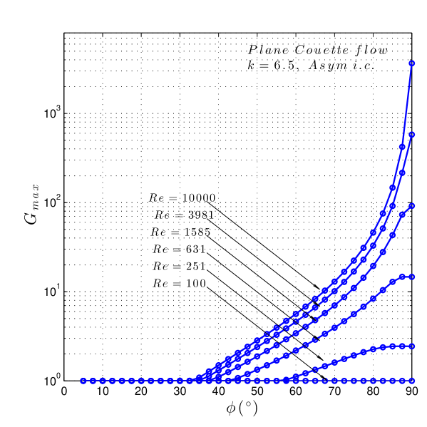
Figure 4.25: Upper plot: maxima of the kinetic energy density $G$ as a function of the obliquity angle $\phi$, parametrized with $Re$, for Plane Couette flow with $k=6.5$ and antisymmetrical initial condition. Lower plot: nondimensional times corresponding the the maxima of $G$. The values of Reynolds number are uniformly distributed in the logarithmic space.

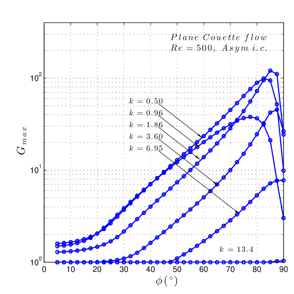
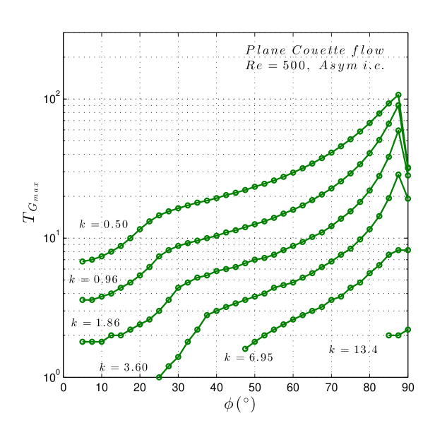
Figure 4.26: Upper plot: maxima of the kinetic energy density $G$ as a function of the obliquity angle $\phi$, parmetrized with $k$, for Plane Couette flow with $Re=500$ and antisymmetrical initial condition. Lower plot: nondimensional times corresponding the the maxima of $G$. The values of polar wavenumber are uniformly distributed in the logarithmic space.

4.3.3   Wave solutions in the physical space

In the following, some solutions among those introduced in §4.3.1 are inverse-transformed using the relations (4.11) and (4.12) to obtain the quantities in the physical space. A few visualizations in the $xy$ plane are here reported (figures 4.27 to 4.30), for the same cases introduced at the end of the previous section, in order to clarify the physical meaning of the module of the complex quantities in the wavenumber space, and to observe the behavior of the flow quantities in the real three-dimensional space. For all the following flow visualizations a variable color scale is adopted to represent at all times the solution, that consequently has to be intended as normalized to its maximum value.

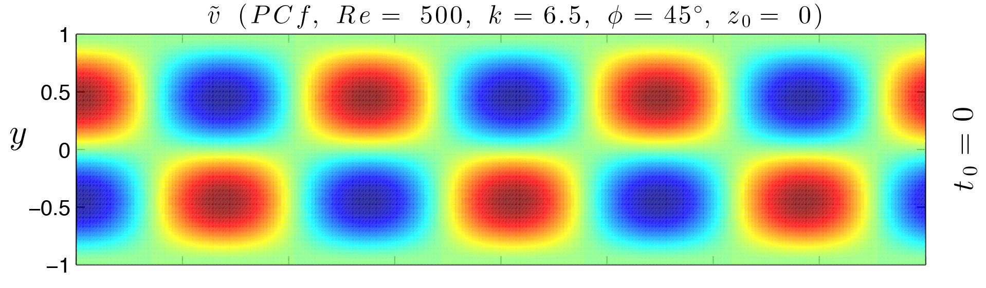
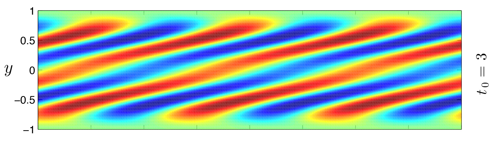
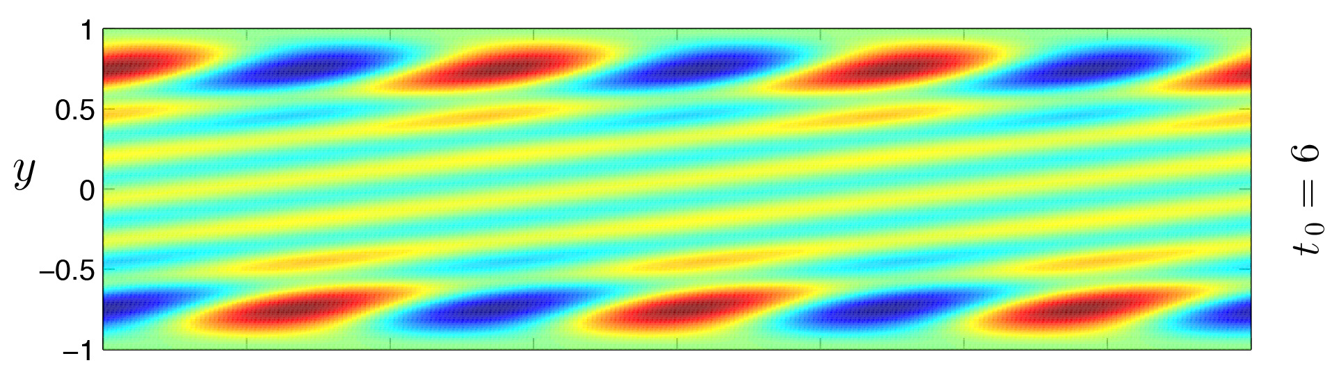
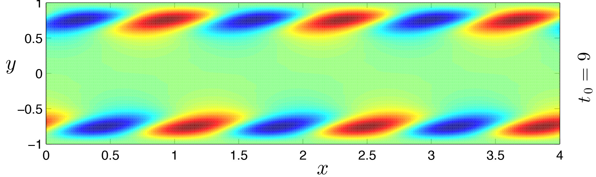
Figure 4.27: Visualization of the wall-normal perturbation velocity $\tilde{v}(x,y,z_{0},t_{0})$, $xy$ plane, for Plane Couette flow with the same parameters of Fig. 4.16. It should be noticed that the $x$-component of the phase velocity takes the same sign of the base flow. Remind that for the adopted conventions the base flow is oriented as the longitudinal axis $x$; with reference to the figure, the upper wall moves to the right, the lower to the left. Red: maximum (positive); blue: minimum (negative).

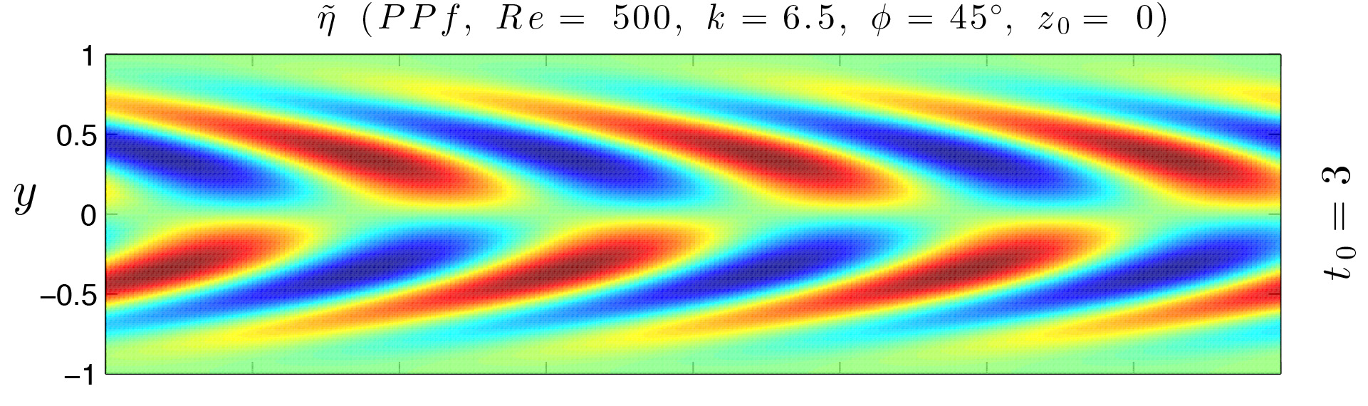
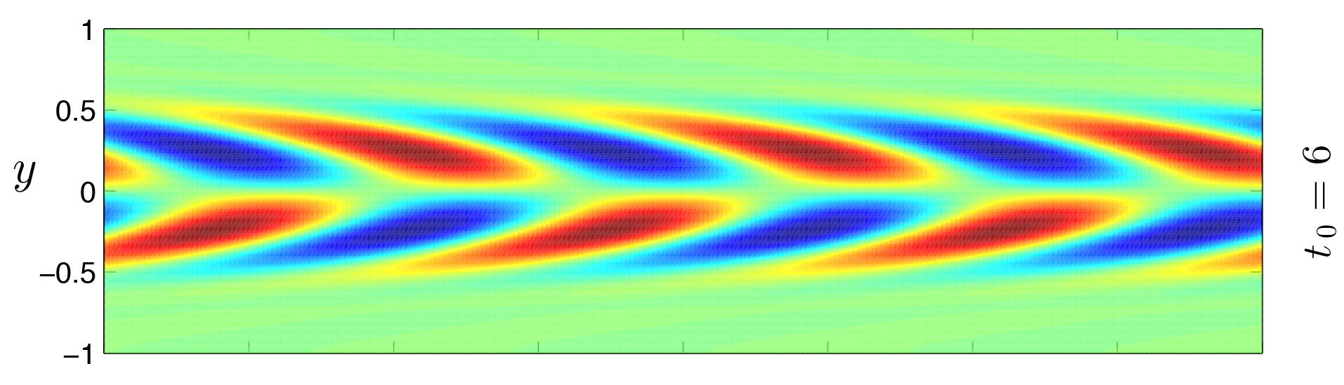
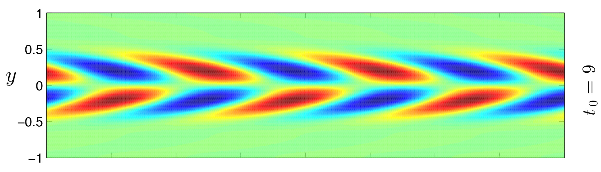
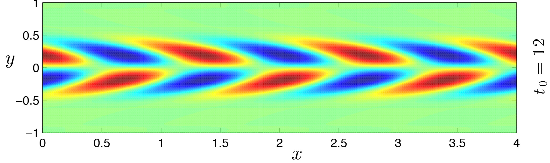
Figure 4.28: Visualization of the wall-normal perturbation vorticity $\tilde{\eta}(x,y,z_{0},t_{0})$, $xy$ plane, for Plane Poiseuille flow. The same parameters of Fig. 4.20 are set, to allow a comparison. From these slices, the disturbance seems to move in the streamwise direction, meaning that the $x$-component of phase velocity has the same sign of the base flow, as observed in Couette flow. Remind that the disturbance direction is defined by the polar wavenumber vector. Red: maximum (positive); blue: minimum (negative).

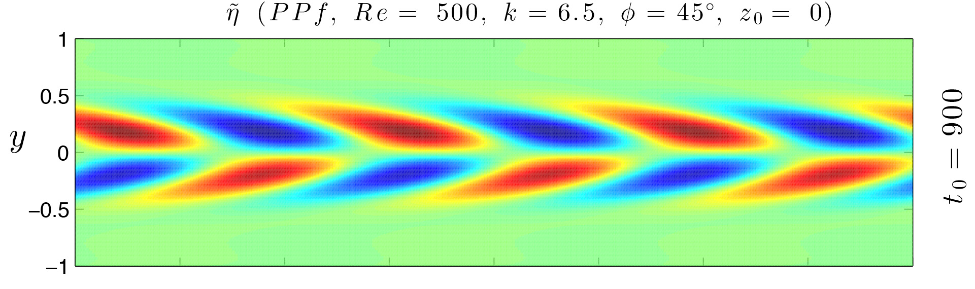
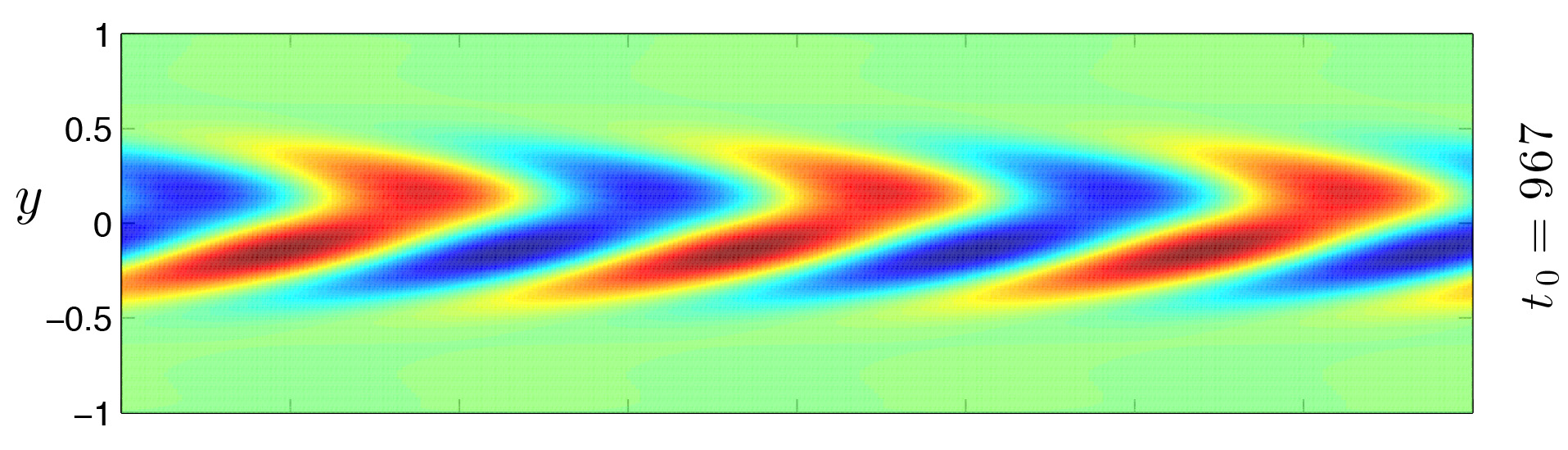
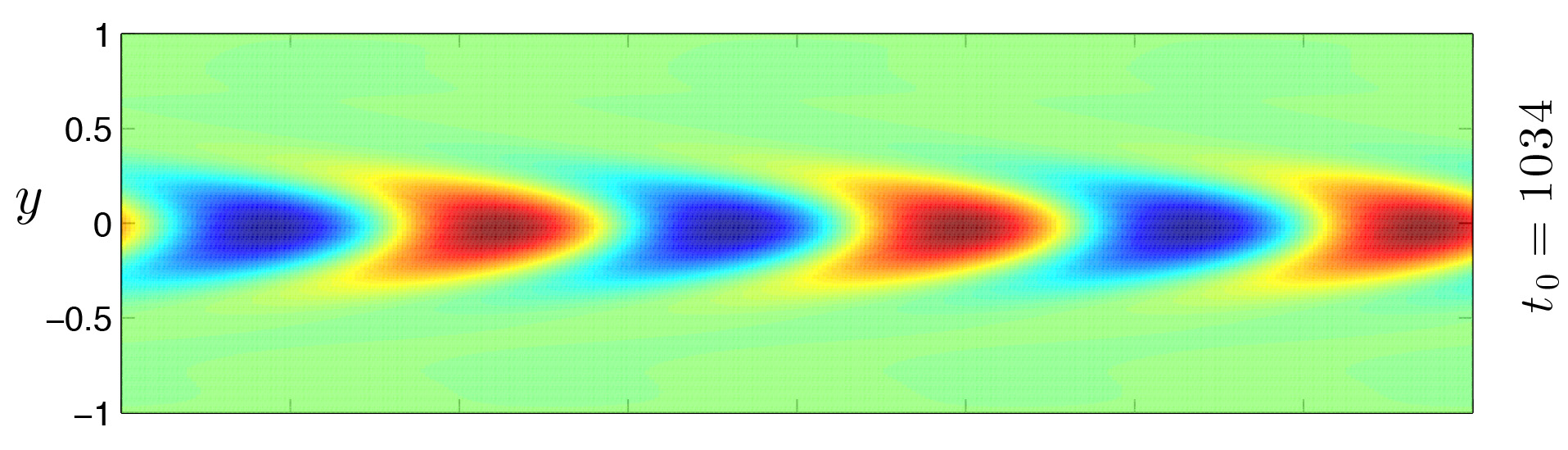
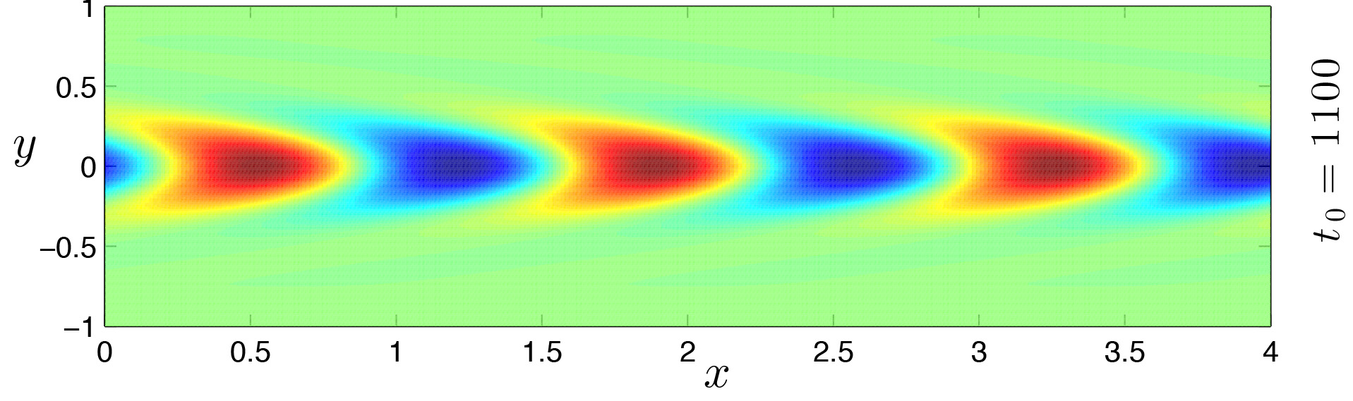
Figure 4.29: Visualization of the wall-normal perturbation vorticity $\tilde{\eta}(x,y,z_{0},t_{0})$, $xy$ plane, for Plane Poiseuille flow. This case correspond to Fig. 4.21, and the effects of the transition to the asymptotic conditions, through the second frequency jump of $\omega_{\eta}$, is shown. Red: maximum (positive); blue: minimum (negative).

Chapter 5       Wave packets linear evolution

5.1   Introduction

In the present chapter the evolution of linear wave packets is investigated. The aim of this study, as stated in the Introduction, is to emphasize the role of the linear mechanisms in a scenario preceding the breakdown and the transition to turbulence. To be more precise, the focus will be on the Plane Couette flow, extensively studied in the previous chapters, and on Blasius boundary layer flow (Bbl, in the following). The wave solutions for the latter are obtained with a Runge-Kutta code by numerical integration of the Orr-Sommerfeld and Squire PDE equations by the method of lines (see Ames, 1977).

Bypass transition and turbulent spots

Although the Plane Couette flow is stable to infinitesimal perturbations for all values of the Reynolds number, experimental evidences showed that for sufficiently high values of $Re$ the flow becomes turbulent. This process is observed in bounded flows and in Bbl as well, and it is known as Bypass transition. The term is due to the fact that this scenario bypasses the growth of two-dimensional waves and their secondary instability. Since this laminar-turbulent transition is observed even for values of the Reynolds number lower than the critical one, obtained by the modal stability theory, many shear flows fall in the class of subcritical transitional flows. The general scenario is the following. The transition does not occur simultaneously in the whole domain, but through nucleation and growth of organized patches of turbulent flow, called turbulent spots, that eventually fill the space. The first observation was made by Emmons (1951) in a water table flow. The PCf has been extensively studied in the past, probably because its zero mean advection speed allows easier tracking of the spots. Experimental investigations has shown the existence of a threshold Reynolds number $Re_{c}$ below which the spots keep a finite probability to relaminarize; among these, we remind the works by Daviaud et al. (1992) ($Re_{c}=370\pm 10$), Tillmark & Alfredsson (1992) ($Re_{c}=360\pm 10$), Hegseth (1996) ($Re_{c}=325$). The most common experimental apparatus consists of a counter-translating belt driven by two rotating cylinders, the working fluid is water and a finite-amplitude disturbance is triggered by fluid injection. Among the nonlinear direct numerical simulations, we report more recent works by Lagha & Manneville (2007), Duguet et al. (2010) ($Re_{c}=324\pm 1$), Duguet et al. (2011) ($Re_{c}=325$). Usually an germ-like initial condition, (typically two counter-rotating vortices), is given in the physical plane. In these cases the authors showed that the turbulent region exhibits elongated flow structures, called streaks, and that for PCf the spot shape is elliptical. When the transition is natural the streaky structure remains, the spots nucleate randomly in space and their shape is more irregular, or oblique bands are found (see Manneville, 2011). The typical distance between two streaks is found to be of the same order of magnitude of the channel half-height, $\lambda_{s}\approx O(h)-O(3h)$. In addition, other typical characteristics of the spot are its propagation speed and spreading rates which depends on the base flow and the Reynolds number. However, for channel flows the spreading of a turbulent spot is quite rapid, if compared to the typical turbulent diffusion: this mechanism is known as “growth by destabilization” of the surrounding laminar flow. Analyzing the structure of the Couette spot, Lundbladth & v. Johansson (1991) and Dauchot & Daviaud (1995) classified it as a case between the Poiseuille and the boundary layer spot.

About the latter, a boundary layer spot is characterized by a horseshoe structure. The complete process of transition on a flat plate with zero pressure gradient has been subject to extensive studies since the beginning of the past century with the work of Burgers (1924) and successively by Tollmien (1929) and Schlichting (1933). Several features distinguish the Bbl transition from the one occurring in internal flows. From the leading edge of the plate, as $x$ increases, the laminar flow is destabilized until the transition zone is reached, where arrowhead turbulent spots appear. A complete description of the structure and the evolution of spots can be found in the experimental works by Cantwell et al. (1978) and Gad-El-Hak et al. (1981). The former also provided beautiful visualizations of both the lateral side of the spot and its bottom side (the sublayer) taking advantage of the glass walls of the water channel. For a complete description of all the boundary layer mechanisms of transition and the onset of turbulence see the review by Kachanov (1994).

Wave packets and role of the linear stages in the transition process

Comparing to the amount of studies about the non-linear stages of transition and the descriptions of the turbulent spots, few investigations are found about the role of the linear evolution of small disturbances in the transitional process. The results of the modal analysis have probably been overestimated, and only recently a renewed interest in the transient evolution of linear three-dimensional disturbances arised. The importance of three-dimensionality and so the spanwise variation of the velocity components was firstly pointed out by the boundary layer experiments by Klebanoff et al. (1962). The instability of this oblique wave develops in $\Lambda$-vortices (K-transition). Zang & Krist (1989) demonstrated that the growth of the oblique waves is correlated with the existence of a mode with $\alpha=0$, i.e. an orthogonal mode. The fact that the presence of this mode is a prerequisite for the rising of secondary instability was confirmed in earlier investigations. Schmid & Henningson (1992) looked at small amplitude wave pairs, and Henningson et al. (1993) devoted to investigating a possible mechanism for bypass transition, pointing out the role of the linear phase and arguing that the mechanism for energy transfer is primarily linear. In fact, the disturbances with no streamwise dependence ($\alpha=0$) are usually those which experience the most rapid growth (see Fig. 4.23-4.26). Henningson et al. (1994) argued the necessity of linear growth mechanisms for subcritical growth of arbitrary amplitude perturbations. Indeed, almost all the Fourier components are contained in a generic initial condition, and those corresponding to the spanwise wavenumber axis are found to be rapidly excited due to linear mechanism. Moreover, even if the initial condition is poor in those components, rapid growth still occurs when non-linear interactions transfer energy in that area of the wavenumber space. The same happens for finite amplitude disturbances: Henningson et al. (1993) pointed out that the energy growth is only caused by the linear mechanism, leading to the streaky horizontal velocity pattern. For subcritical flows this means that the transient growth effect must operate for transition to take place.

The streaky structure, typical of various flow configurations, is also related to the evolution of optimal (in a linear sense) disturbances, which can arise and bring to nonlinearity (see e.g. Brandt et al., 2003). In fact, the wall-normal shape of linearly optimal disturbances determined by Andersson et al. (1999) is surprisingly similar to the measured $u_{rms}$ values. We should also cite the work by Cherubini et al. (2010), who looked for optimal initial conditions and also made a comparison between a linear and a nonlinear analysis of a spot evolution in Bbl. They shows that the streaky structure and the general shape of the spot are already determined by the linear analysis, due to the kinetic energy transient growth. Only in the following nonlinear phase, secondary instability of the streaks occurs and the spot central region becomes turbulent.

5.2   Linear spot in Plane Couette flow

The results of the linear superposition of a large number of waves are shown in Fig. 5.1-5.4. The purpose of these visualizations is to confirm the role of the linear transient dynamics in the complex transitional scenario, showing that in the evolution of a wave packet some of the typical features of a transitional flow may be encountered. Differently from the works by the cited authors, here a localized disturbance is simply obtained by a superposition, with zero phase-shift, of a large number of waves with obliquity angle $\phi$ spanning the full circle. The polar wavenumber $k$ is restricted to a few values chosen accordingly to the experimental evidences found in literature. For Plane Couette flow the chosen values are $k=\{5.7,\ 6.5,\ 7.3\}$, while the Reynolds number is $500$, with reference to the experimental work by Hegseth (1996). Both odd and even initial condition (the same introduced and used in the previous chapters) are considered. The solutions to the initial value problem  (3.1)-(3.2) are inverse-transformed, according to the relations (4.11) and (4.12), and then superimposed, so the complete flow field in an arbitrary domain in $x$ and $z$ directions can be easily obtained. If an in-phase superposition of a large number of waves is considered, a bump-like initial condition in the physical space is obtained, as shown in Fig. 5.2. Clearly, if the considered domain is wide enough, a repetitive periodic scheme can be observed. The equivalence with a two-dimensional Fourier transform is straightforward. Hence, this procedure is a simple way to qualitatively represent a localized perturbation in the physical space, containing the contributions of all obliquity angles. Moreover, correlations with the transient evolution of single waves, shown in Chapter 4, are possible.

In the following, the results are reported in terms of the three components of velocity $\tilde{u}$, $\tilde{v}$, $\tilde{w}$, and the pointwise kinetic energy $\tilde{e}(x,y,z,t)=0.5*({\tilde{u}}^{2}+{\tilde{w}}^{2}+{\tilde{w}}^{2})$. Remind that the amplitude of the initial perturbation does not have any influence on the results, since the analysis is linear. That is the reason why all the reported fields are normalized to the maximum value gained at $t=0$. For Plane Couette flow is convenient to visualize the quantities at the channel symmetry plane $y=0$, since the mean flow is zero. The first stages of the evolution of the linear spot seem to be characterized by a dominant spanwise rate of spreading, due to the faster waves with $\beta\to 0$. When the orthogonal wave ($\alpha=0$) becomes dominant, a streaky flow structure is found: note that a negative band of the component $\tilde{u}$ corresponds to a positive one of $\tilde{v}$.

In order to show the evolution of the initial perturbation in the three-dimensional domain, the open-source VisIt tool has been used. A Matlab^® script has been written to create the VTK file needed by VisIt, and the points structured grid format has been used. In Fig. 5.5, isosurfaces of streamwise velocity are shown.

Streamwise velocity - Plane Couette flow, $Re=500$

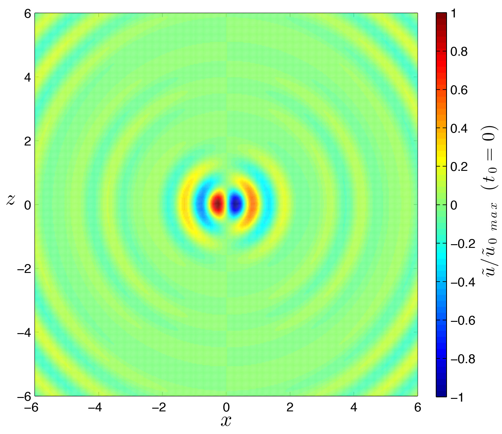
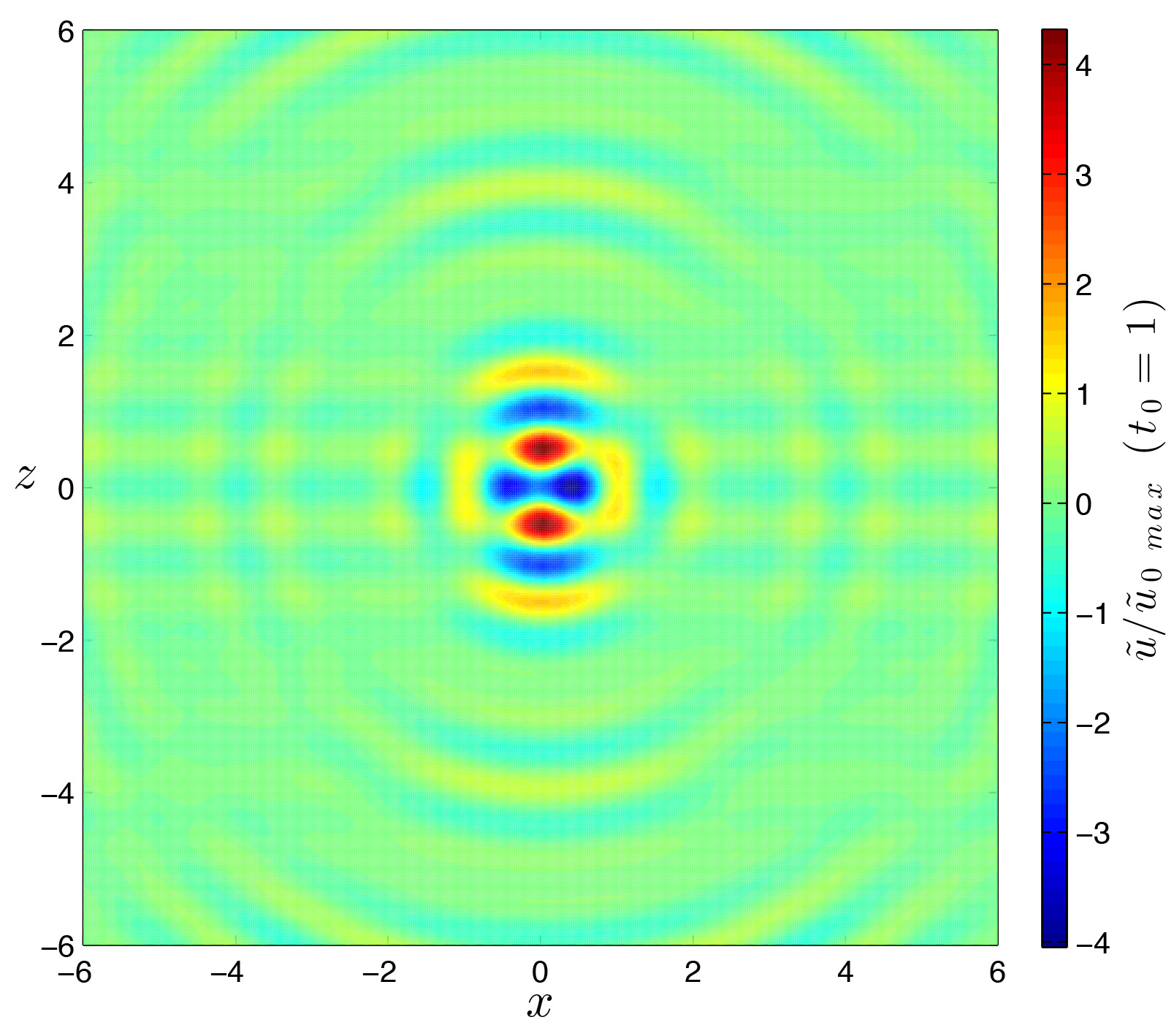
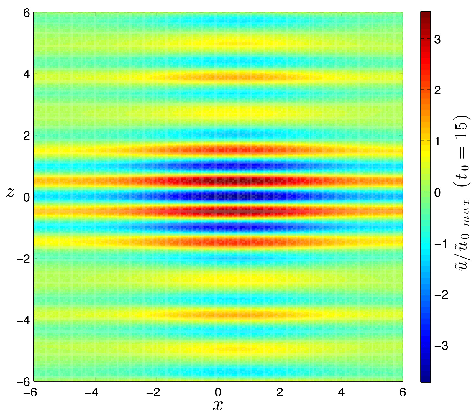
Figure 5.1: Visualization of longitudinal velocity $\tilde{u}$ for PCf with $Re=500$. Views of $xz$ plane at the channel symmetry plane at different times. The evolution of a localized perturbation is obtained by superposition of 220 waves with polar wavenumber $k=\{5.7,\ 6.5,\ 7.3\}$, obliquity angle spanning the full circle, $\phi\in\{-90^{\circ},\ +90^{\circ}\}$, with both sym and asym initial conditions. The values are normalized with respect to the maximum at time $t=0$.

Wall-normal velocity - Plane Couette flow with $Re=500$

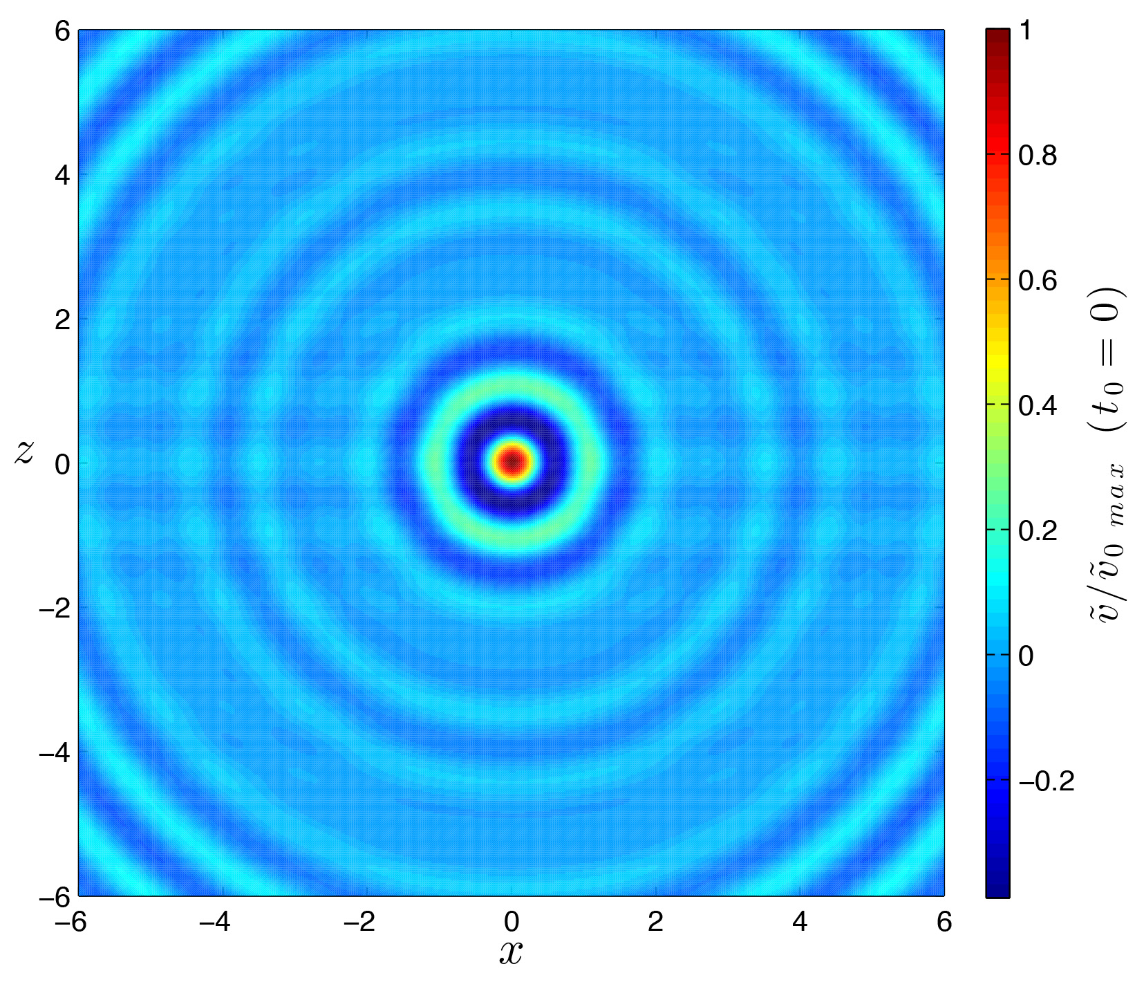
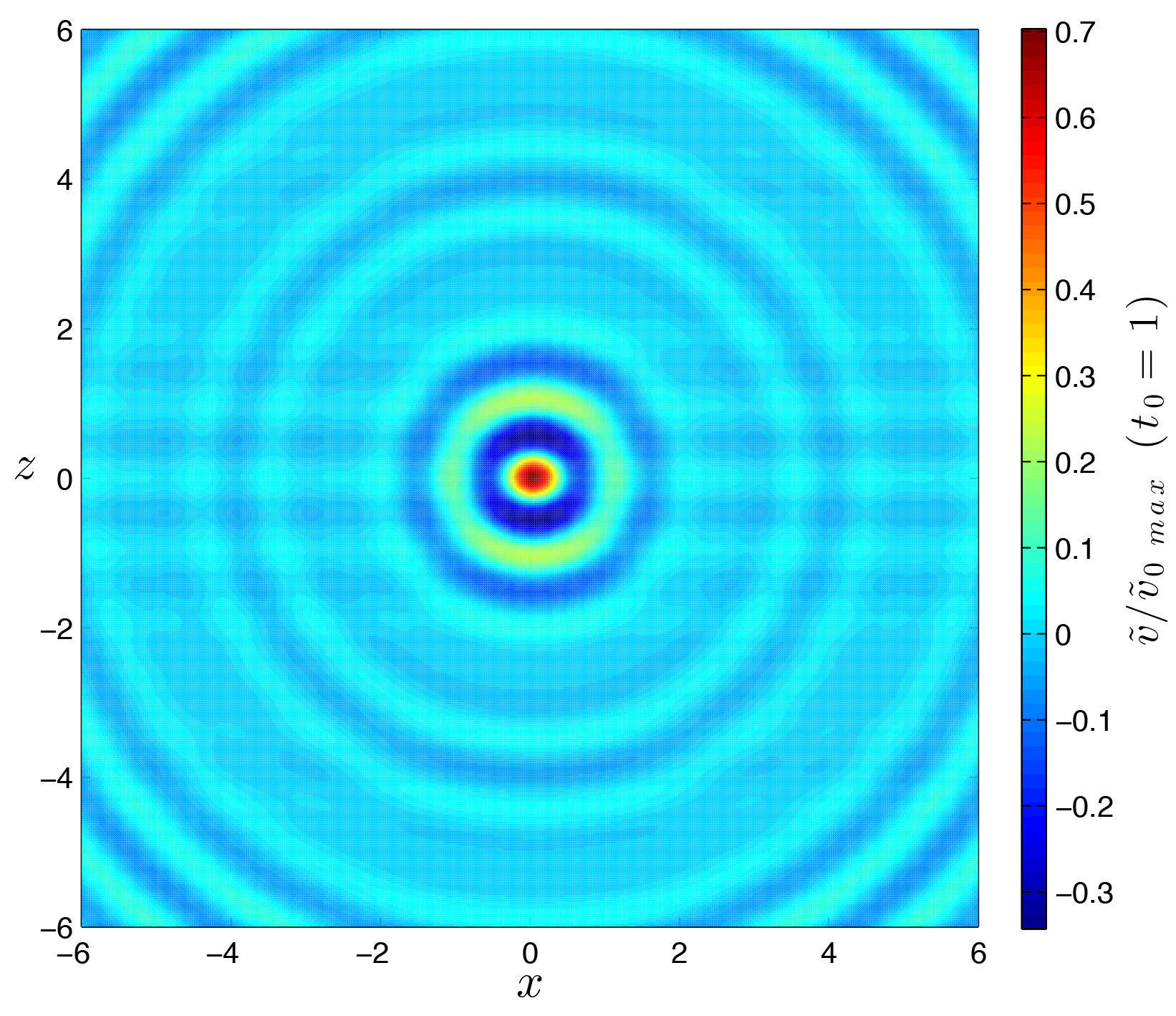
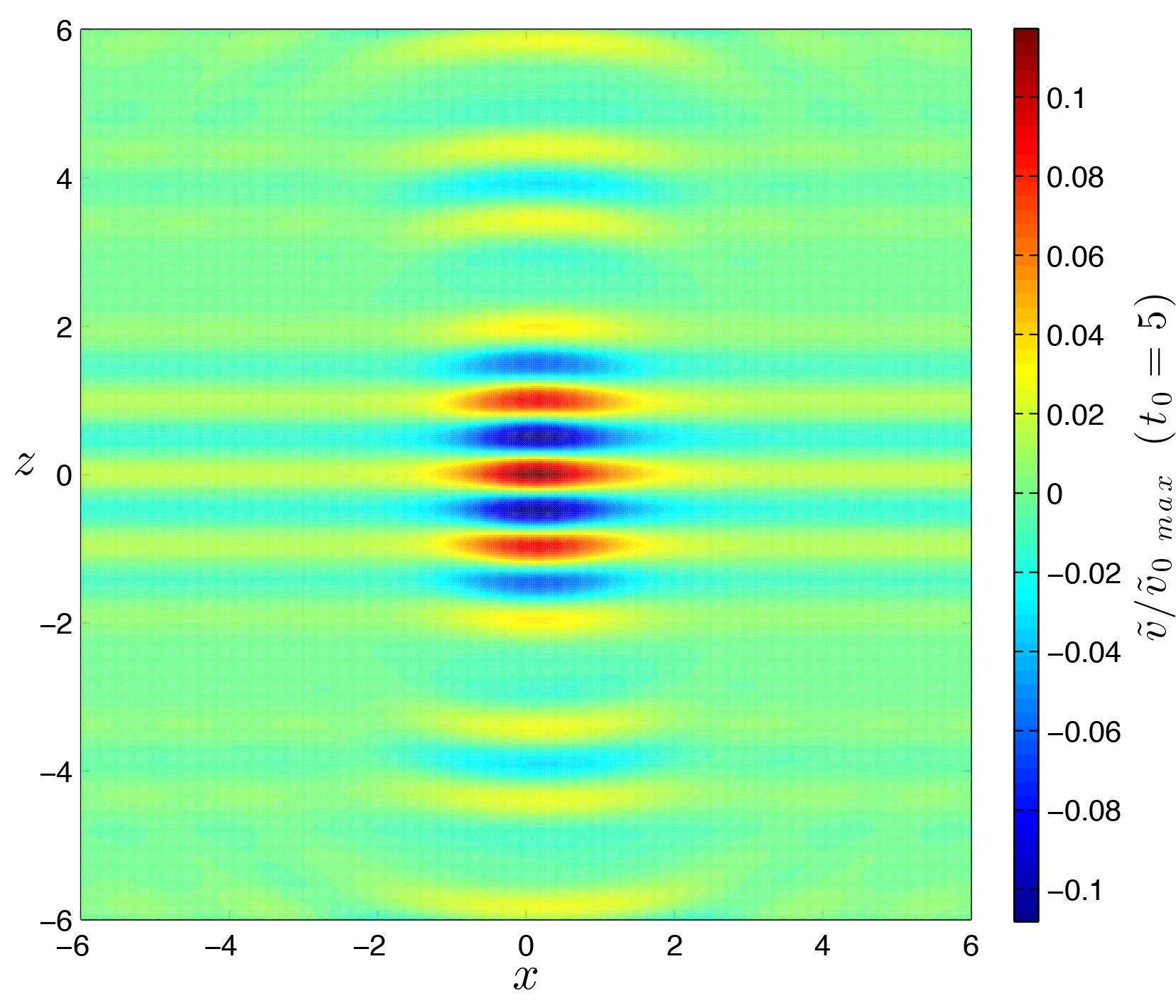
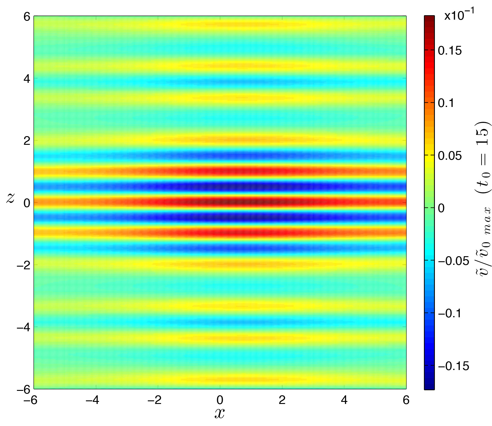
Figure 5.2: Visualization of the wall-normal velocity $\tilde{v}$ for PCf with $Re=500$. Views of $xz$ plane at the channel symmetry plane at different times. The evolution of a localized perturbation is obtained by superposition of 220 waves with polar wavenumber $k=\{5.7,\ 6.5,\ 7.3\}$, obliquity angle spanning the full circle, $\phi\in\{-90^{\circ},\ +90^{\circ}\}$, with both sym and asym initial conditions. The values are normalized with respect to the maximum at time $t=0$.

Spanwise velocity - Plane Couette flow with $Re=500$

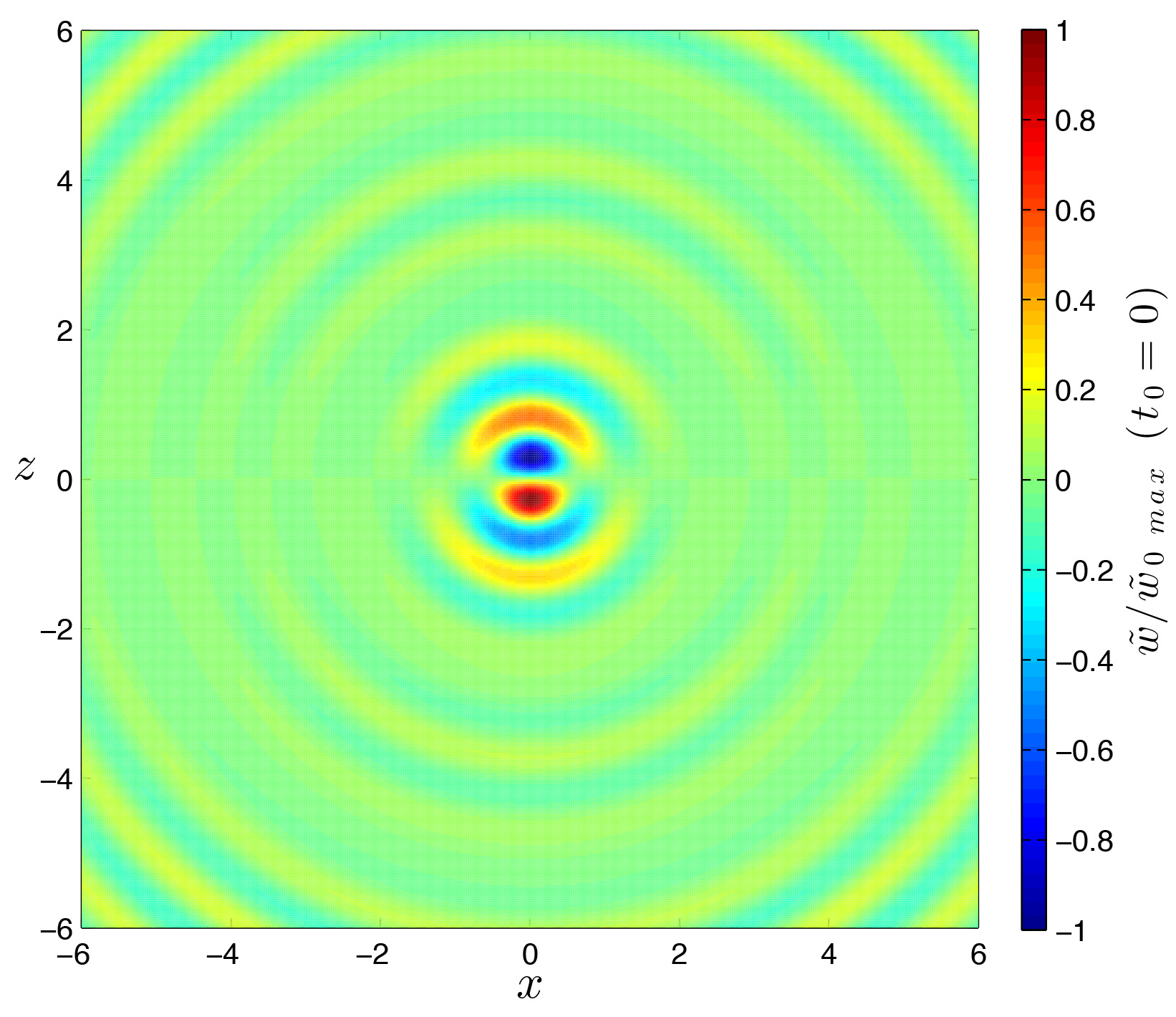
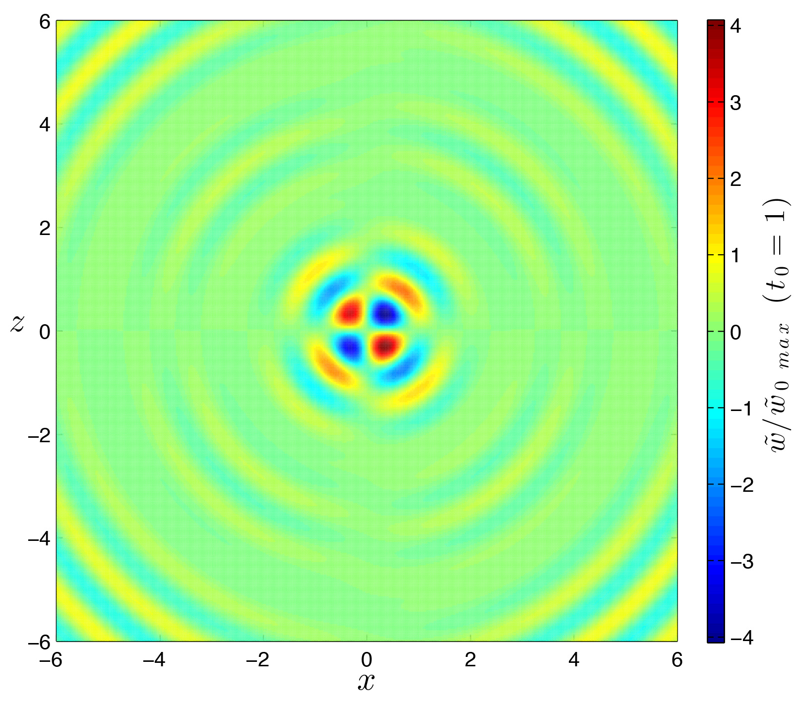
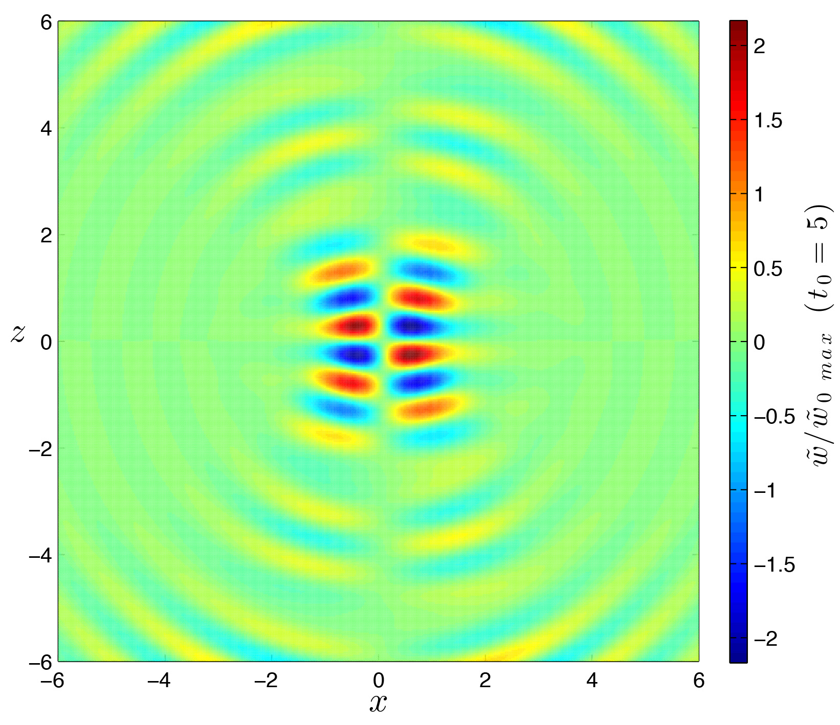
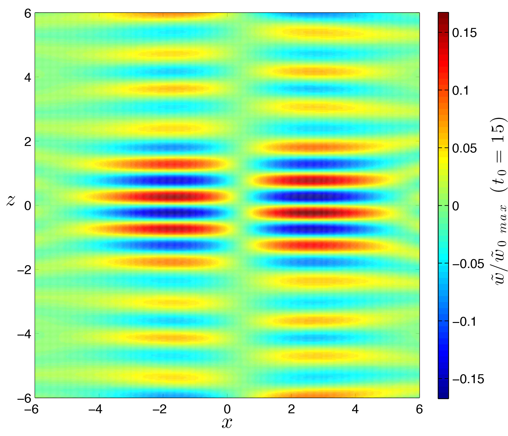
Figure 5.3: Visualizations of the spanwise velocity $\tilde{w}$ for PCf with $Re=500$. Views of $xz$ plane at the channel symmetry plane at different times. The evolution of a localized perturbation is obtained by superposition of 220 waves with polar wavenumber $k=\{5.7,\ 6.5,\ 7.3\}$, obliquity angle spanning the full circle, $\phi\in\{-90^{\circ},\ +90^{\circ}\}$, with both sym and asym initial conditions. The values are normalized with respect to the maximum at time $t=0$.

Kinetic energy - Plane Couette flow with $Re=500$

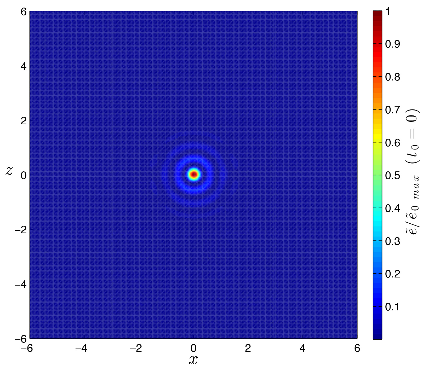
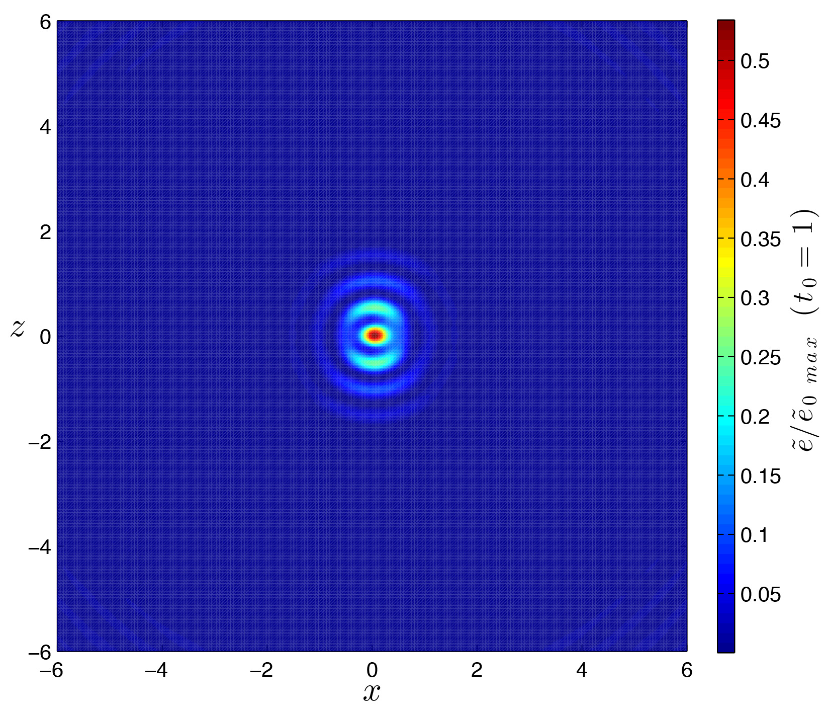
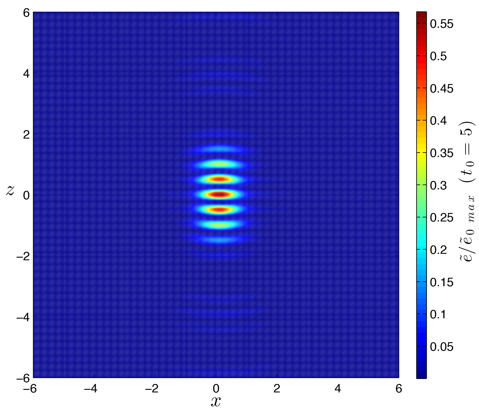
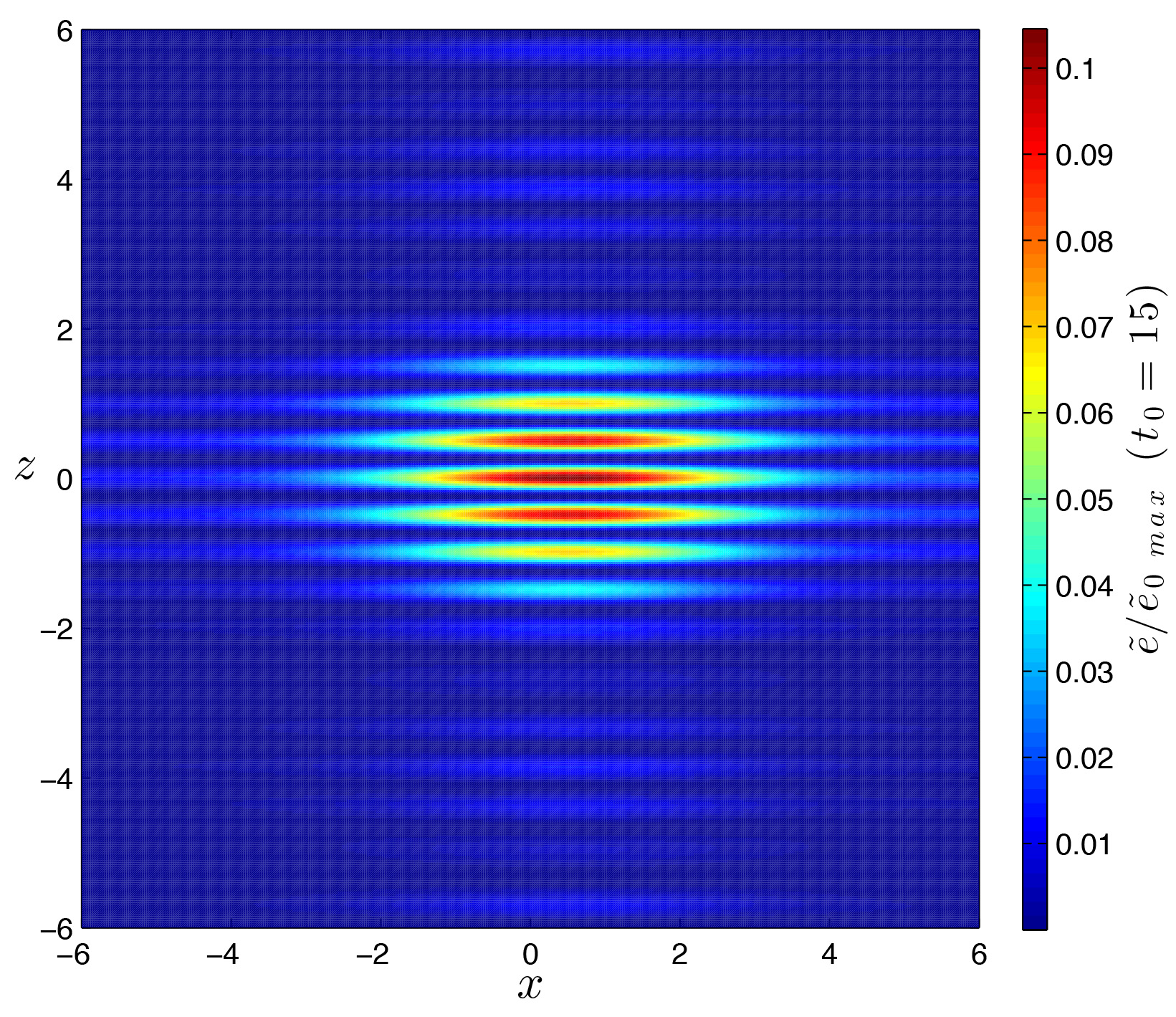
Figure 5.4: Visualization of the kinetic energy $\tilde{e}$ for PCf with $Re=500$. Views of $xz$ plane at the channel symmetry plane at different times. The evolution of a localized perturbation is obtained by superposition of 220 waves with polar wavenumber $k=\{5.7,\ 6.5,\ 7.3\}$, obliquity angle spanning the full circle, $\phi\in\{-90^{\circ},\ +90^{\circ}\}$, with both sym and asym initial conditions. The values are normalized with respect to the maximum at time $t=0$.

3D visualization of streamwise velocity, PCf with $Re=500$

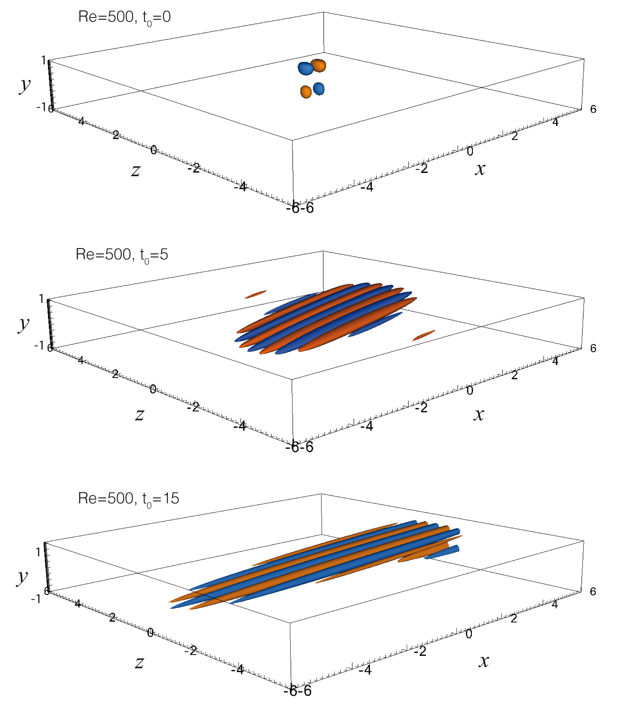
Figure 5.5: 3D visualization of streamwise velocity for PCf with $Re=500$. (a) Initial condition, $t_{0}=0$; orange surface: $\tilde{u}/{\tilde{u}}_{0\ max}=0.5$; blue surface: $\tilde{u}/{\tilde{u}}_{0\ max}=-0.5$; (b) $t_{0}=5$; orange surface: $\tilde{u}/{\tilde{u}}_{0\ max}=1$; blue surface: $\tilde{u}/{\tilde{u}}_{0\ max}=-1$; (b) $t_{0}=15$; orange surface: $\tilde{u}/{\tilde{u}}_{0\ max}=1$; blue surface: $\tilde{u}/{\tilde{u}}_{0\ max}=-1$. Here ${\tilde{u}}_{0\ max}$ is the maximum value in the whole 3D domain at the initial time (${\tilde{u}}_{0\ max}=20.8$). Remind that the upper wall moves in the $x$ direction, and the lower wall moves in the opposite direction. As can be noticed, the initial perturbation is stretched, resulting in a streaky structure which is inclined with respect to the symmetry plane of the channel.

5.3   Linear spot in Blasius boundary-layer flow

Concluding the present work, the evolution of a localized perturbation in boundary-layer flow is shown. The base flow here considered is the one corresponding to a flat plate with zero incidence (Blasius boundary-layer, see e.g. Schlichting, 1979; Rosenhead, 1963). The chosen value for Reynolds number, defined with the displacement thickness is 1000, while five values of the polar wavenumber are considered, $k=\{1.26,\ 1.57,\ 2.09,\ 3.14,\ 6.28\}$. Remind also that the spatial coordinates are here normalized with the displacement thickness, while the reference velocity is the free stream velocity $U_{\infty}$. Simulations have been performed with two different initial conditions in order to get a wide database with a variety of transient behaviors, whose expressions are the following

$$\hat{v}_{0}^{(1)}=y^{2}e^{-y^{2}}\ \ \ \ \hat{\eta}_{0}^{(1)}=0$$ (5.1)

$$\hat{v}_{0}^{(2)}=y^{2}e^{-y^{2}}sin(\pi y)\ \ \ \ \hat{\eta}_{0}^{(2)}=0$$

The former is always positive while the latter is oscillating, they both satisfy the boundary conditions and have their maximum near the wall, inside the boundary layer. Also for this case, the evolution of a localized disturbance obtained by in-phase superposition is shown. The total number of considered waves is 365. However, some trials have been made with a smaller number of waves, randomly chosen, leading to the same general conclusions. In these cases, a more irregular shape of the spot is observed. The affinity of the shape acquired by the wave packet with the one of a turbulent spots, is noticeable (see e.g. Fig. 5.6): the initial disturbance evolves elongating mainly in the streamwise direction, and a $\Lambda$-structure can be clearly observed. Even from noisy or dynamic initial condition cases, carried out by random waves superposition or random inputs in time (not presented in this work), it is possible to observe a flow field dominated by not exactly rectilinear streaks, and often a $\Lambda$ - pattern can be recognised.
Also in the case of Bbl, the origin of the $x$ and $z$ axis for non-dimensional coordinates is considered to be the location of the initial disturbance (see e.g. Fig. 5.6a). The three-dimensional evolution of the linear spot can be observed from Fig. 5.10, where isosurfaces for the streamwise velocity are shown. The qualitative behaviour is in agreement with the one recently shown by Cherubini et al. (2010).
Finally, in Tab. 5.1 we report the results for a dimensional case with $U_{\infty}=15m/s$ and $\nu=1.45\cdot 10^{-5}$ (air flow). This is helpful for understanding the true order of magnitude of the quantities involved.

Streamwise velocity - Blasius boundary layer flow with $Re=1000$

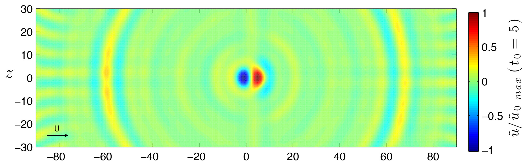
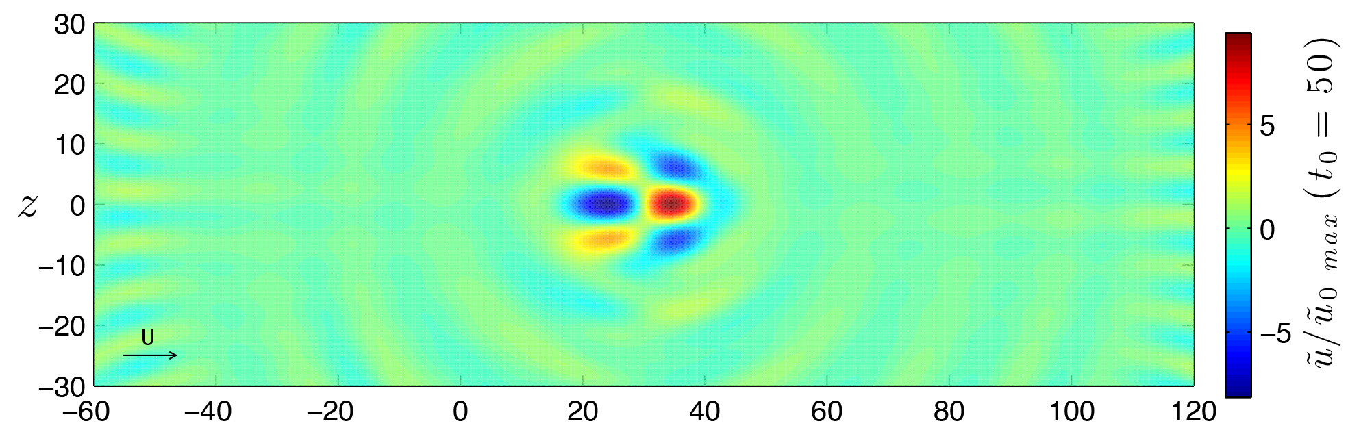
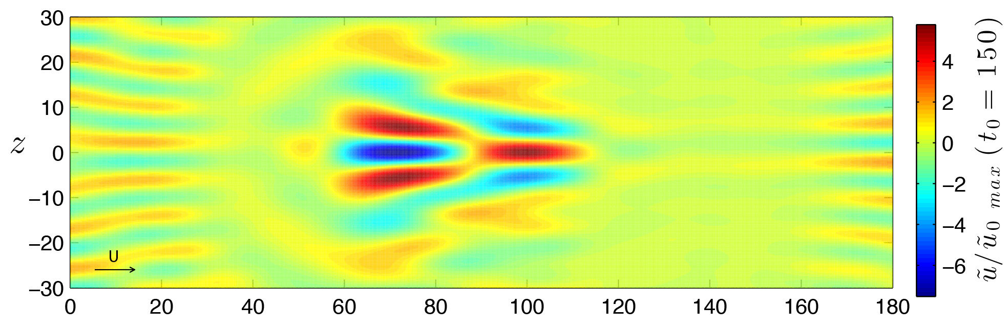
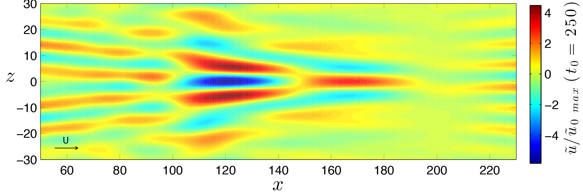
Figure 5.6: Visualizations of the longitudinal velocity $\tilde{u}$ for Bbl with $Re=1000$. Views of $xz$ plane at $y_{0}=1.5$. The evolution of a localized perturbation is obtained by superposition of 365 waves with polar wavenumber $k=\{1.26,\ 1.57,\ 2.09,\ 3.14,\ 6.28\}$, obliquity angle spanning the full circle, $\phi\in\{-90^{\circ},\ +90^{\circ}\}$, and two different initial conditions. Remind that the mean flow moves in the right direction.

Wall-normal velocity - Blasius boundary layer flow with $Re=1000$

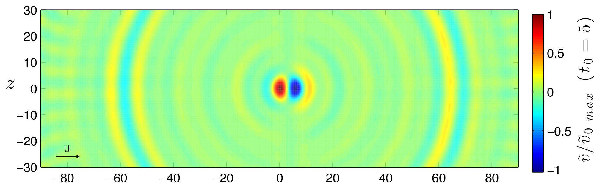
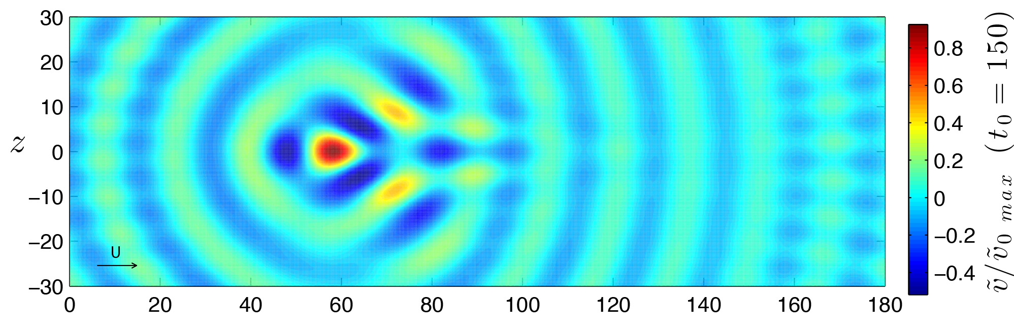
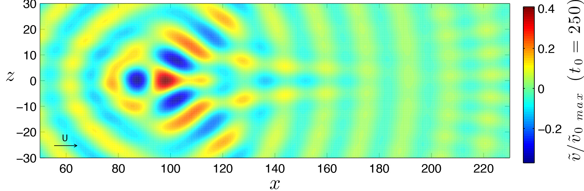
Figure 5.7: Visualizations of the wall-normal velocity $\tilde{v}$ for Bbl with $Re=1000$. Views of $xz$ plane at $y_{0}=1.5$. The evolution of a localized perturbation is obtained by superposition of 365 waves with polar wavenumber $k=\{1.26,\ 1.57,\ 2.09,\ 3.14,\ 6.28\}$, obliquity angle spanning the full circle, $\phi\in\{-90^{\circ},\ +90^{\circ}\}$, and two different initial conditions.

Spanwise velocity - Blasius boundary layer flow with $Re=1000$

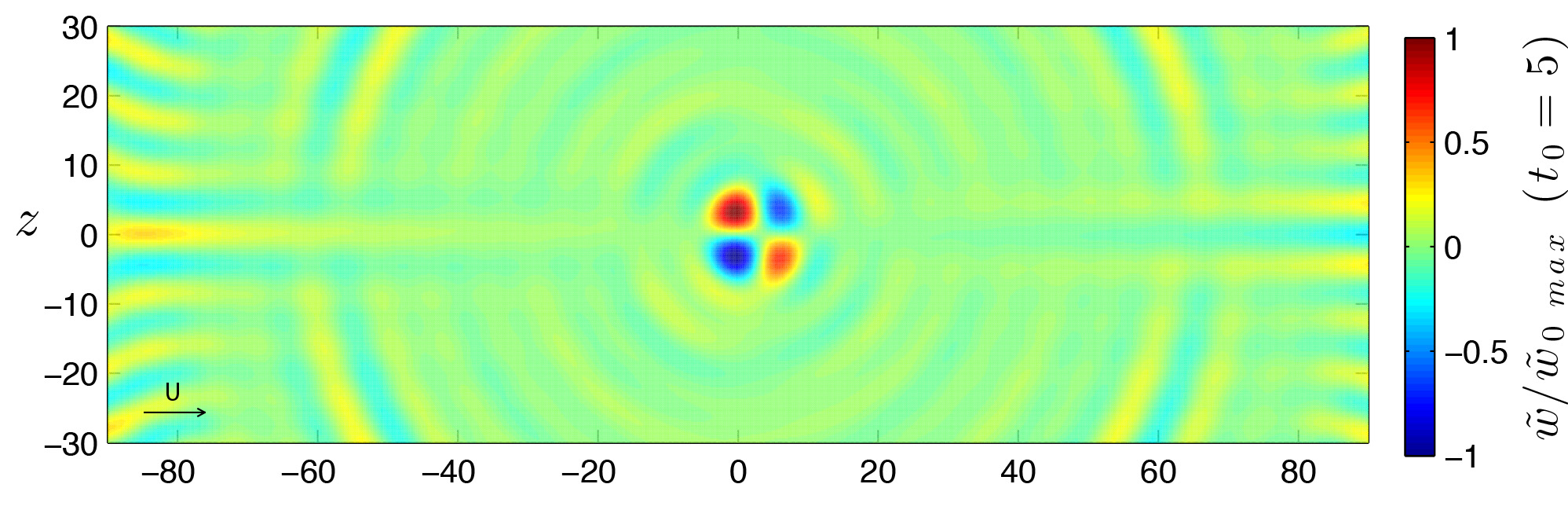
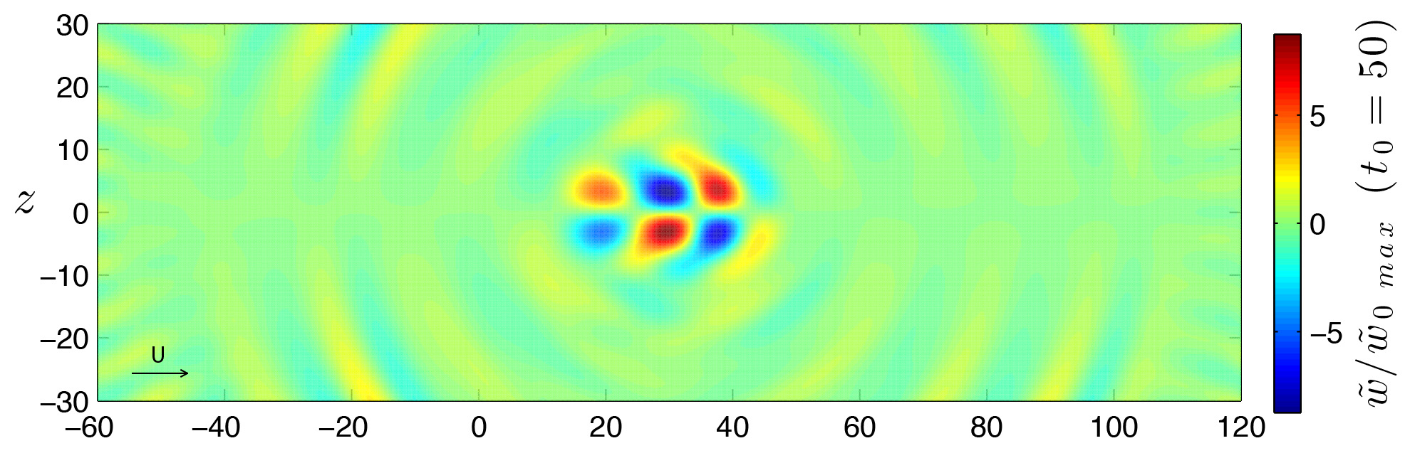
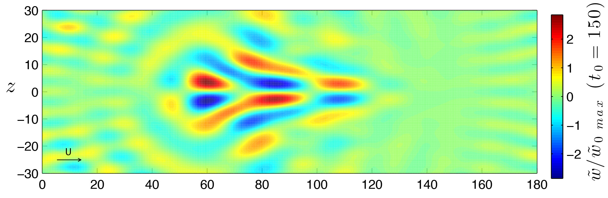
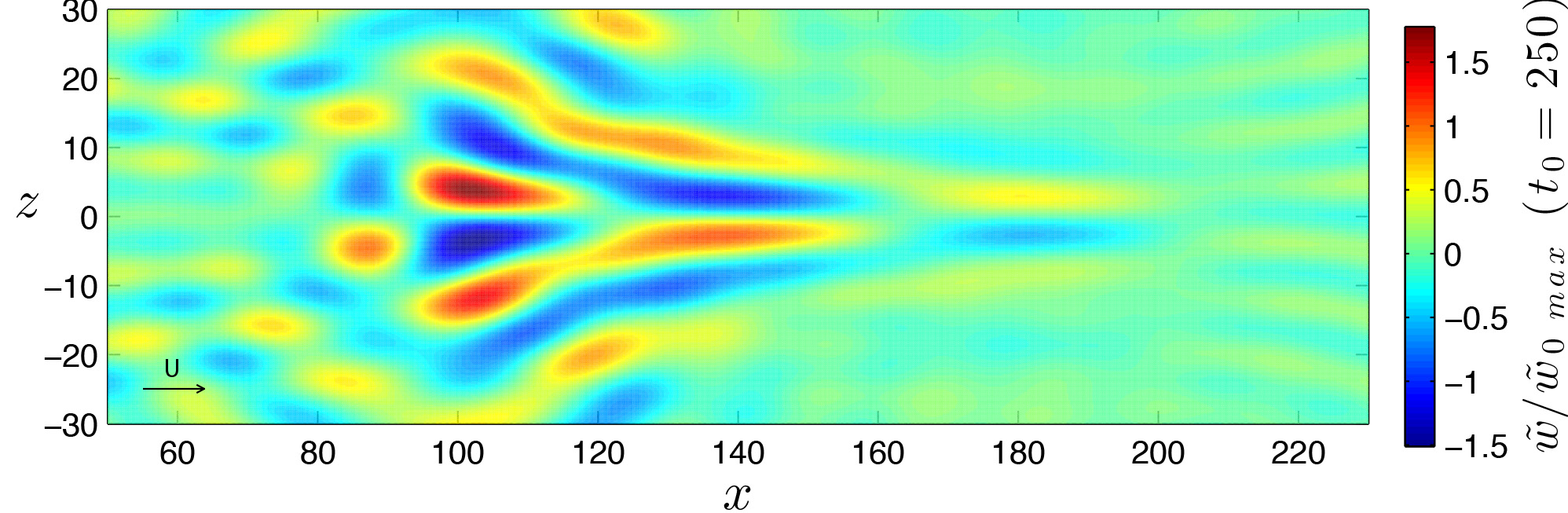
Figure 5.8: Visualizations of the spanwise velocity $\tilde{w}$ for Bbl with $Re=1000$. Views of $xz$ plane at $y_{0}=1.5$. The evolution of a localized perturbation is obtained by superposition of 365 waves with polar wavenumber $k=\{1.26,\ 1.57,\ 2.09,\ 3.14,\ 6.28\}$, obliquity angle spanning the full circle, $\phi\in\{-90^{\circ},\ +90^{\circ}\}$, and two different initial conditions.

Kinetic energy - Blasius boundary layer flow with $Re=1000$

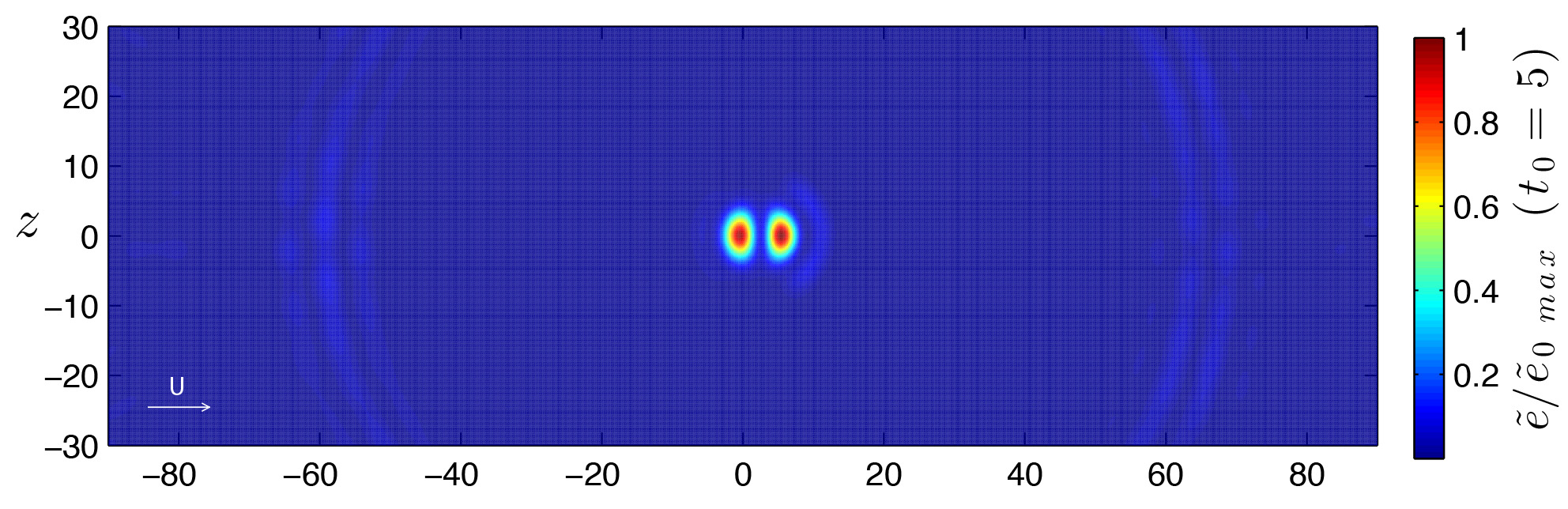
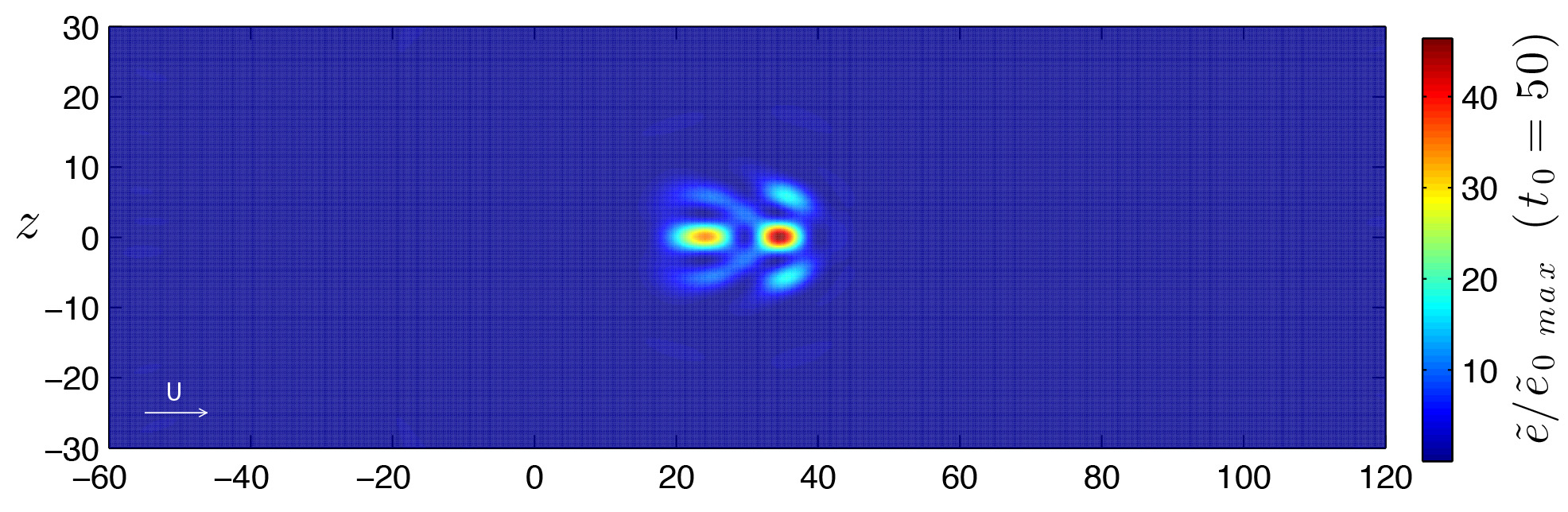
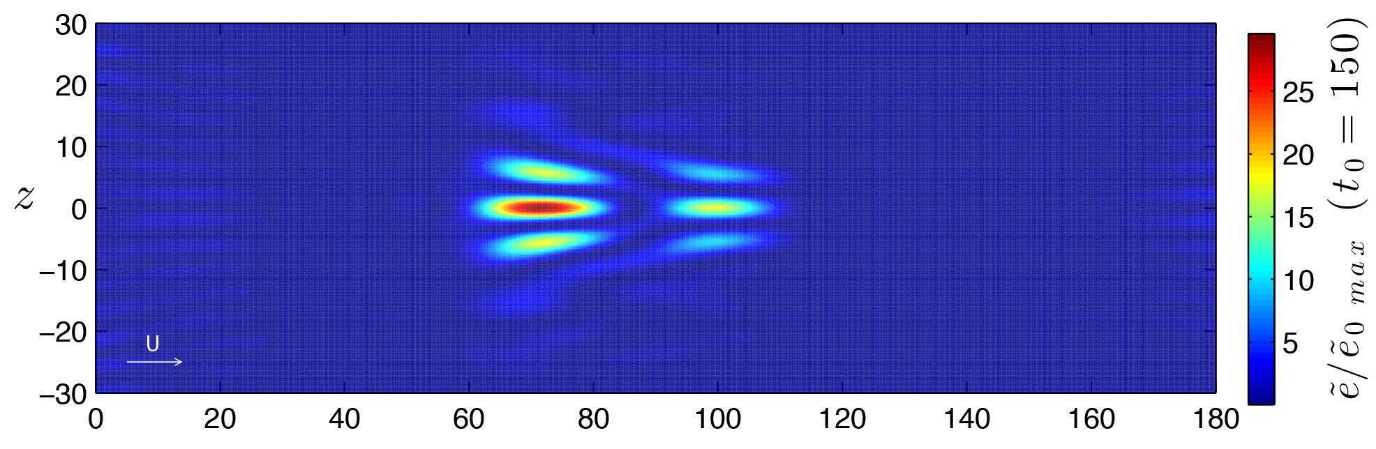
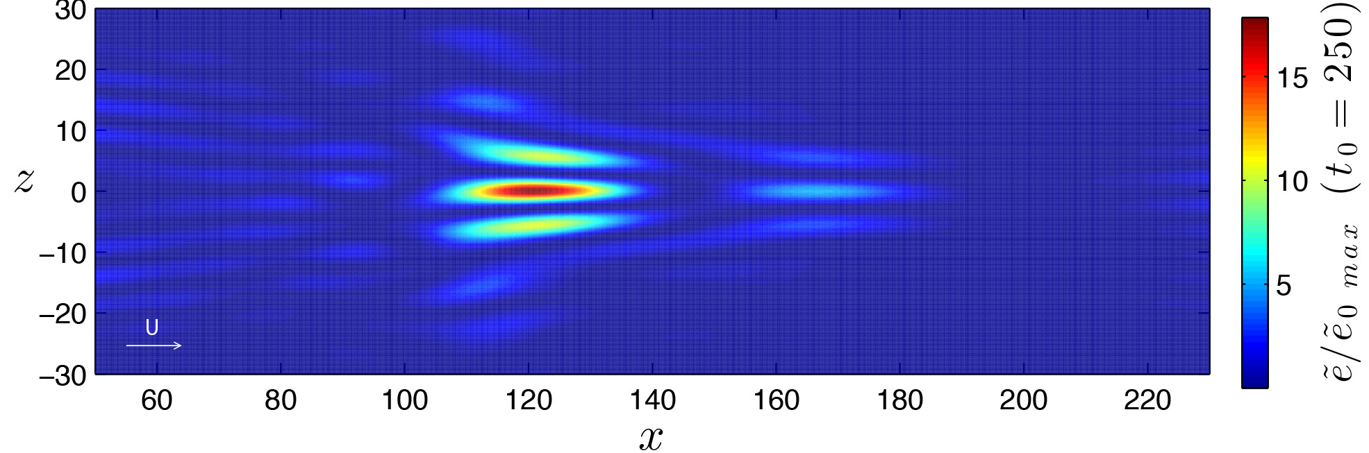
Figure 5.9: Kinetic energy visualizations for Bbl with $Re=1000$. Views of $xz$ plane at $y_{0}=1.5$. The evolution of a localized perturbation is obtained by superposition of 365 waves with polar wavenumber $k=\{1.26,\ 1.57,\ 2.09,\ 3.14,\ 6.28\}$, obliquity angle spanning the full circle, $\phi\in\{-90^{\circ},\ +90^{\circ}\}$, and two different initial conditions.

3D visualization of streamwise velocity, Bbl with $Re=1000$

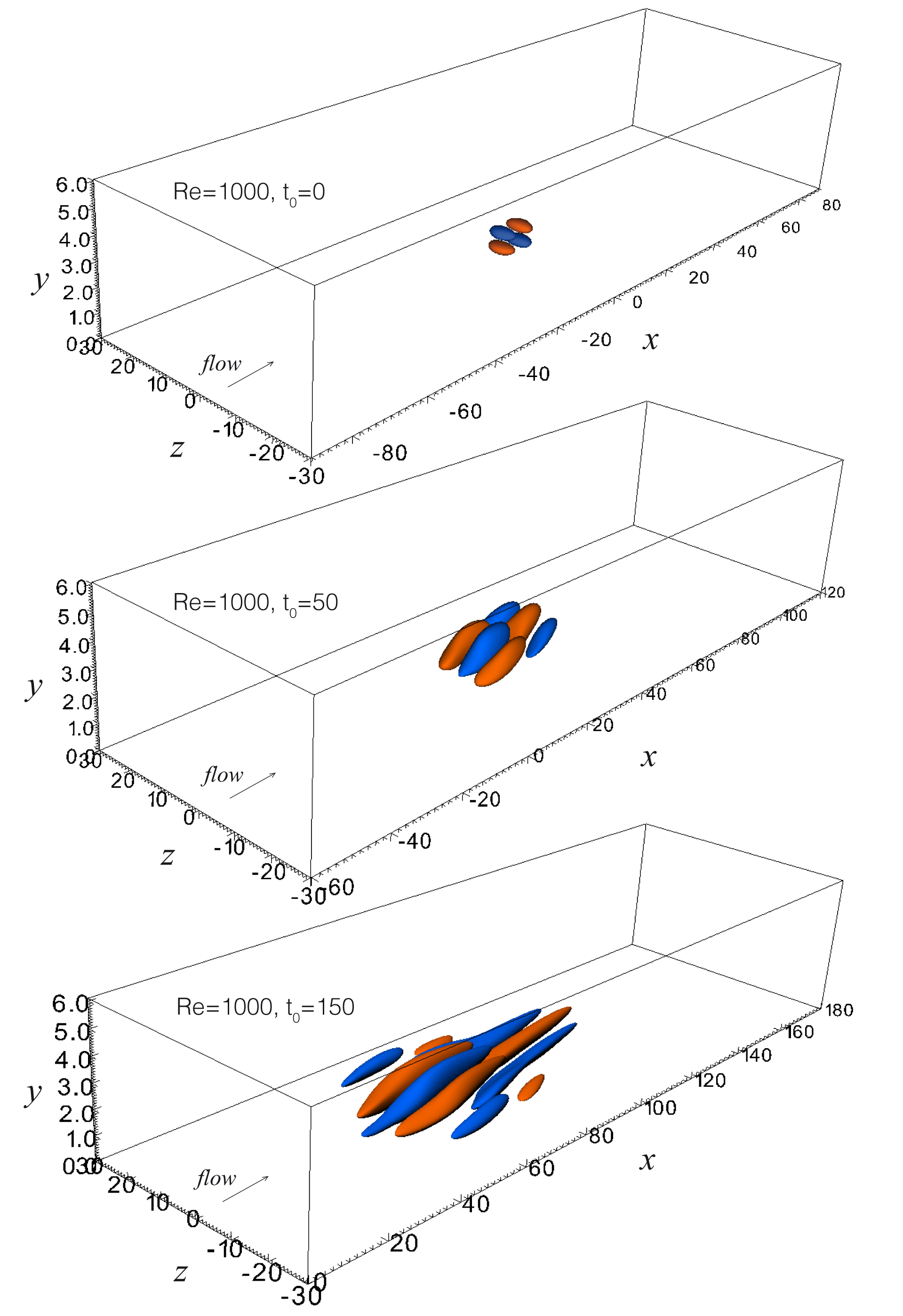
Figure 5.10: 3D visualization of streamwise velocity for Bbl with $Re=1000$. (a) Initial condition, $t_{0}=0$; orange surface: $\tilde{u}/{\tilde{u}}_{0\ max}=0.5$; blue surface: $\tilde{u}/{\tilde{u}}_{0\ max}=-0.5$; (b) $t_{0}=50$; orange surface: $\tilde{u}/{\tilde{u}}_{0\ max}=1$; blue surface: $\tilde{u}/{\tilde{u}}_{0\ max}=-1$; (b) $t_{0}=150$; orange surface: $\tilde{u}/{\tilde{u}}_{0\ max}=1$; blue surface: $\tilde{u}/{\tilde{u}}_{0\ max}=-1$. Here ${\tilde{u}}_{0\ max}$ is the maximum value in the whole 3D domain at the initial time (${\tilde{u}}_{0\ max}=214$).

In the following table, a summary of the linear spot evolution for the analyzed case is shown, and also the dimensional quantities are reported for a specific case with $U_{\infty}=15m/s$ and air flow ($\nu=1.45\cdot 10^{-5}$). In this conditions, a Reynolds number of 1000 is found at a distance $x-x_{le}=328$ mm from the leading edge of the flat plate, where $\delta^{*}=0.97$ mm. This is considered the origin of the non-dimensional $x$ axis, where the linear spot is triggered. Actually, in the evolution of the perturbation the boundary-layer thickness and the Reynolds number change, but in this analysis the approximation of nearly-parallel flow applies. In Tab. 5.1 $x_{c}$ is the location of the center of the spot, $U_{c}$ is the longitudinal velocity of the spot center, $L_{x}$ and $L_{z}$ are the longitudinal and spanwise sizes for $y_{0}=1.5$, respectively. All these quantities are esteemed from visualizations of the streamwise perturbation velocity.

	$t=0$	$t=5$	$t=50$	$t=150$	$t=250$
	$\mathrm{𝟎}$ ms	$0.323$ ms	$32.3$ ms	$9.70$ ms	$16.2$ ms
$\delta^{*}$	$0.967$ mm	$0.972$ mm	$1.01$ mm	$1.08$ mm	$1.16$ mm
$\delta_{0.99}$	$2.770$ mm	$2.773$ mm	$2.88$ mm	$3.08$ mm	$3.31$ mm
$x_{c}$	0	2	29.6	88.0	148
	$328$ mm	$330$ mm	$357$ mm	$413$ mm	$471$ mm
$U_{c}$	0	0.8	0.67	0.64	0.64
	$0$ m/s	$12$ m/s	$10$ m/s	$9.6$ m/s	$9.6$ m/s
$L_{x}$	6	12	25	60	94
	$5.82$ mm	$11.6$ mm	$24.3$ mm	$58.2$ mm	$91.2$ mm
$L_{z}$	6	12	18	24	24
	$5.82$ mm	$11.6$ mm	$17.5$ mm	$23.3$ mm	$23.3$ mm

Table 5.1: Dimensional quantities for the evolution of a localized perturbation in a Blasius boundary-layer flow with $Re=1000$. The approximation of nearly-parallel flow is applied, in fact the Reynolds number for every simulation is fixed. It can be noticed that the true spatial and temporal scales are quite small.

Chapter 6       Conclusions

The present work deals with the hydrodynamic stability non-modal analysis. In the first part, a close form solution to the three-dimensional Orr-Sommerfeld and Squire IVP in the form of orthogonal functions expansion was researched. The Galerkin variational method was then successfully implemented in the Matlab^® environment to numerically compute approximate solutions to the coupled equations, for bounded flows. The Chandrasekhar functions revealed to ensure a convergence rate scaling as $N^{5}$ to the correct solution even for the non-modal analysis. The advantages of this method can be summarized in the independence of the accuracy on both the temporal and spatial grids, which can be considered arbitrary, and the very low time computational cost. Moreover, since there is no “marching” in time, no stiffness problems are encountered and accurate solutions can be obtained up to very high times. The spectra of the Orr-Sommerfeld and Squire operators are computed with high precision, as well.

The code has been intensively used to focus on the temporal evolution of the wave frequency and phase velocity, poorly investigated in the past. The results confirmed recent observations about the frequency jump in the $\tilde{v}$ component of flow velocity, considered as the end of the Early transient. After this first jump, the frequency of $\tilde{v}$ for Plane Couette flow experiences a periodic modulation about the asymptotic value, which has been motivated and investigated in detail.

A new result is the presence of a second jump in the phase velocity of the vorticity component $\tilde{\eta}$ and consequently of the other components of velocity, typically for high times. The presence of a second jump and the possibility for different values of asymptotic frequency of the signals were motivated and no contradictions with the results of the modal theory subsist. This is the proof of the existence of an Intermediate transient, in fact, only after the last jump the solution reaches its asymptotic state. Moreover, a connection between the frequency jumps and the establishing of a self-similarity condition in time for both the velocity and vorticity profiles was found and investigated for both Plane Couette flow and Plane Poiseuille flow. The behavior in the physical space was also shown.

The last result deals with the linear evolution of wave packets. Through superposition of waves with limited wavenumber range a wave packet is reconstructed for Plane Couette flow and Blasius boundary-layer flow. The structure of the linear spot revealed to have many common features with the early stages of a turbulent spot, particularly the streaky structure and the shape. This is in agreement with recent ideas and observations and supports the thesis of the underrated importance of the linear mechanisms such as the transient growth, in the transitional scenario.

Appendix A

A.1   The basis eigenfunctions

The solutions of the problem (3.9) with homogeneous boundary conditions (3.10) can be found by seeking a solution of the following form

$$X(y)=C_{1}e^{\lambda y}+C_{2}e^{-\lambda y}+C_{3}e^{i\lambda y}+C_{4}e^{-i\lambda y}$$ (A.1)

where $C_{i}$ are constants. Since we are interested in real eigenfunctions, the above expression becomes

$$X(y)=Asinh(\lambda y)+Bcosh(\lambda y)+Csin(\lambda y)+Dcos(\lambda y)$$ (A.2)

where $A$, $B$, $C$ and $D$ are constants, to be determined. Substituting the solution in the expressions of the boundary conditions, a system of four algebraic equations where the constant are the unknown is found. The following relations are obtained

$$A=-C\frac{sin(\lambda)}{sinh(\lambda)}\hskip 28.45274ptB=-D\frac{cos(\lambda)}{cosh(\lambda)}$$ (A.3)

$$\begin{bmatrix}-\tfrac{sin(\lambda)}{tanh(\lambda)}+cos(\lambda)&-cos(\lambda)tanh(\lambda)-sin(\lambda)\\ -\tfrac{sin(\lambda)}{tanh(\lambda)}+cos(\lambda)&cos(\lambda)tanh(\lambda)+sin(\lambda)\end{bmatrix}\begin{pmatrix}C\\ D\end{pmatrix}=\begin{pmatrix}0\\ 0\end{pmatrix}$$ (A.4)

Nontrivial solution to the system (A.4) are possible if the determinant of the coefficients matrix vanishes, this leads to the equation

$$tan^{2}(\lambda)-tanh^{2}(\lambda)=0$$ (A.5)

from which the couple of trascendental equations (3.11) and (3.12) are derived. The solution to these equations consists in two sets of infinite and discrete eigenvalues $\lambda_{n}$, that can be computed numerically by the bisection or the Newton-Raphson method (Fig. A.1). In Tab. A.1 the first twenty eigenvalues are shown.

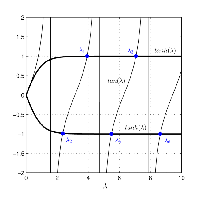
Figure A.1: Graphic solution of the eigenvalue problem (A.4). Odd indices indicate the eigenvalues corresponding to odd eigenfunctions and even indices correspond to even eigenfunctions. Since both sets are antisymmetric with resprect to $\lambda=0$ axis, only positive eigenvalues are considered.

$n$	$\lambda_{n\ (odd)}$
1	3.926602
3	7.068582
5	10.21017
7	13.35176
9	16.49336
11	19.63495
13	22.77654
15	25.91813
17	29.05973
19	32.20132

(a) Odd eigenvalues

$n$	$\lambda_{n\ (even)}$
2	2.365020
4	5.497803
6	8.639379
8	11.78097
10	14.92256
12	18.06415
14	21.20575
16	24.34734
18	27.48893
20	30.63052

(b) Even eigenvalues

Table A.1: First 20 eigenvalues, numerically computed using the Newton-Raphson method.

Appendix B

B.1   Matlab^® scripts for channel flows Galerkin method

B.1.1   Main program: “main_ivp_galerkin.m”

⬇

1%% IVP SOLUTION BY GALERKIN METHOD for Channel flows

2% The stability IVP is reduced to an ODE system and solved by

3% Galerkin variational method.

4clear all,close all,clc

5tic

6%% Simulation parameters

7global tol N U DU D2U type Re k_polar alfa beta phi ss y y_ic t

8type=’Couette’;

9Re=500;␣␣␣␣␣␣␣␣%␣Reynolds␣number

10k_polar=6.5;␣␣␣%␣Polar␣wavenumber

11phi=5;␣␣␣␣␣␣␣␣␣%␣Obliquity␣perturbation␣angle

12alfa=k_polar*cosd(phi);

13beta=k_polar*sind(phi);

14ss=’sym’;␣␣␣␣␣␣%␣Type␣of␣initial␣condition

15h=0.01;

16y=-1:h:1;␣␣␣␣␣␣␣%␣Grid␣for␣solution

17y_ic=-1:1e-4:1;␣%␣Fine␣grid␣for␣initial␣condition␣computaiton

18N=200;␣␣␣␣␣␣␣␣␣␣%␣Num.␣of␣eigenmodes␣chosen␣for␣calculation␣(must␣be␣even).

19tol=1e-10;␣␣␣␣␣␣%␣Tolerance␣for␣error␣checking.

20col=colormap(jet(15));

21y0=0.5;

22temp=find(y>=y0);

23idxy=temp(1);

24dt=0.5;

25t=0:dt:100;␣␣␣␣␣%␣Time␣grid

26

27disp␣’%%%%%%%%%%%%%%%%%%%%%%%%%%%%%%%%%%%%%%%%%%%%%%%%%%%%%%%%%%%%%%%%%%%%’

28disp([’Simulation␣of␣Plane␣’,num2str(type),’␣flow’])

29disp([’Re=␣’,num2str(Re),’,␣k_polar=␣’,num2str(k_polar),’,␣phi=␣’,…

30␣␣␣␣␣num2str(phi),’␣deg,␣’,num2str(ss),’␣Initial␣Condition.’])

31disp([’N=␣’,num2str(N),’␣eigenfunctions’])

32disp␣’%%%%%%%%%%%%%%%%%%%%%%%%%%%%%%%%%%%%%%%%%%%%%%%%%%%%%%%%%%%%%%%%%%%%’

33

34%%␣Base␣flow␣definition

35if␣strcmp(type,’Couette’)==1

36␣␣␣␣U=y;

37␣␣␣␣DU=1;

38␣␣␣␣D2U=0;

39elseif␣strcmp(type,’Poiseuille’)==1

40␣␣␣␣U=(1-y.^2);

41␣␣␣␣DU=-2*y;

42␣␣␣␣D2U=-2;

43end

44

45%————————————————————————-%

46%%␣NORMAL-VELOCITY␣SOLUTION␣v(y,t)

47%————————————————————————-%

48%%␣Eigenmodes␣computation

49%␣The␣chosen␣base␣of␣functions␣is␣composed␣by␣two␣set␣of␣eigenfuncions␣of

50%␣the␣problem␣X_yyyy=lam^4*X␣with␣b.c.␣X(-1)=X(1)=X’(-1)=X’(1)=0.

51%␣One␣set␣is␣made␣of␣odd␣modes,␣the␣other␣contains␣even␣modes.␣Both␣sets␣are

52%␣necessary␣to␣obtain␣a␣correct␣solution␣of␣the␣3D␣problem,␣independently

53%␣on␣the␣parity␣of␣the␣initial␣condition.

54%␣Here␣we␣put␣togheter␣the␣two␣set␣in␣following␣order:[1o␣1e␣2o␣2e␣3o␣3e…]

55%(e=even,␣o=odd),␣and␣the␣corresponding␣eigenvalues␣are␣ordered␣in␣this

56%sequence␣too.␣See␣"compute_eigenvalues.m"␣for␣their␣computation.

57

58load␣’eigenvalues.mat’;%␣"eigenvalues.mat",␣contains␣the␣eigenvalues

59␣␣␣␣␣␣␣␣␣␣␣␣␣␣␣␣␣␣␣␣␣␣␣%corresponding␣to␣form␣functions.

60g=gtot(1:N);␣␣␣␣␣␣␣␣␣␣␣%␣g␣are␣the␣eigenvalues.

61

62eigenmodes=zeros(length(g),length(y));

63D1eigenmodes=zeros(length(g),length(y));␣%␣first␣derivatives␣of␣eigenmodes

64D2eigenmodes=zeros(length(g),length(y));␣%␣second␣derivatives␣of␣eigenmodes

65for␣i=1:length(g)

66␣if␣mod(i,2)==1␣%␣odd␣eigenfuncion

67␣␣eigenmodes(i,:)=1/sqrt(2)*(sinh(g(i)*y)/sinh(g(i))-sin(g(i)*y)/sin(g(i)));

68␣␣eigenmodes_ic(i,:)=1/sqrt(2)*(sinh(g(i)*y_ic)/sinh(g(i))-sin(g(i)*y_ic)/sin(g(i)));

69␣␣D1eigenmodes(i,:)=g(i)/sqrt(2)*(cosh(g(i)*y)/sinh(g(i))-cos(g(i)*y)/sin(g(i)));

70␣␣D2eigenmodes(i,:)=g(i)^2/sqrt(2)*(sinh(g(i)*y)/sinh(g(i))+sin(g(i)*y)/sin(g(i)));

71␣elseif␣mod(i,2)==0␣%␣even␣eigenfuncion

72␣␣eigenmodes(i,:)=1/sqrt(2)*(cosh(g(i)*y)/cosh(g(i))-cos(g(i)*y)/cos(g(i)));

73␣␣eigenmodes_ic(i,:)=1/sqrt(2)*(cosh(g(i)*y_ic)/cosh(g(i))-cos(g(i)*y_ic)/cos(g(i)));

74␣␣D1eigenmodes(i,:)=g(i)/sqrt(2)*(sinh(g(i)*y)/cosh(g(i))+sin(g(i)*y)/cos(g(i)));

75␣␣D2eigenmodes(i,:)=g(i)^2/sqrt(2)*(cosh(g(i)*y)/cosh(g(i))+cos(g(i)*y)/cos(g(i)));

76␣end

77end

78

79%%␣Computation␣of␣coefficients␣Cn0,␣from␣prescribed␣initial␣condition

80if␣strcmp(ss,’sym’)==1

81␣␣␣␣ic=(1-y.^2).^2;

82␣␣␣␣ic_a=(1-y_ic.^2).^2;␣␣␣␣%␣symmetric␣initial␣condition

83elseif␣strcmp(ss,’asym’)==1

84␣␣␣␣ic=(1-y.^2).^2;

85␣␣␣␣ic_a=y.*(1-y_ic.^2).^2;␣%␣asymmetric␣initial␣condition

86end

87

88A=zeros(1,N);

89approx_ic=zeros(1,length(y));

90Cn0=zeros(1,N);

91for␣i=1:N;

92␣␣␣␣num=trapz(y_ic,ic_a.*eigenmodes_ic(i,:));

93␣␣␣␣den=1;

94␣␣␣␣Cn0(i)=num/den;

95␣␣␣␣approx_ic(1,:)=␣approx_ic(1,:)+Cn0(i)*eigenmodes(i,:);

96end

97

98%%␣Computation␣of␣matrices␣D␣S␣F␣U1␣U2␣U3␣H␣G

99%␣ODE␣system␣is␣[H]{dc/dt}-[G]{c}=0

100D=zeros(N,N);

101S=zeros(N,N);

102H=zeros(N,N);

103F=zeros(N,N);

104U1=zeros(N,N);

105U2=zeros(N,N);

106G=zeros(N,N);

107H=zeros(N,N);

108

109%%␣D␣and␣F

110Dnm=zeros(1,N);

111Fnm=zeros(1,N);

112for␣i=1:N

113␣␣␣␣Dnm(i)=1;

114␣␣␣␣Fnm(i)=Dnm(i)*g(i)^4;

115end

116D=diag(Dnm,0);

117F=diag(Fnm,0);

118

119bbb=(cosh(2*g)-cos(2*g))./(sinh(2*g)-sin(2*g));

120idNaN=find(isnan(bbb)==1);

121bbb(idNaN)=1;

122S=zeros(N,N);

123

124for␣m=1:N

125␣␣␣␣for␣n=1:N

126␣␣␣␣␣␣␣␣%%␣S

127␣␣␣␣␣␣␣␣if␣mod((m+n),2)==0␣&&␣n~=m

128␣␣␣␣␣␣␣␣␣␣␣␣S(m,n)=+4*g(n)^2*g(m)^2/(g(n)^4-g(m)^4)*(g(n)*bbb(n)-g(m)*bbb(m));

129␣␣␣␣␣␣␣␣elseif␣mod((m+n),2)==1␣&&␣n~=m

130␣␣␣␣␣␣␣␣␣␣␣␣S(m,n)=0;

131␣␣␣␣␣␣␣␣elseif␣n==m

132␣␣␣␣␣␣␣␣␣␣␣␣S(m,n)=-(g(n)^2*bbb(n)^2-g(n)*bbb(n));

133␣␣␣␣␣␣␣␣end

134

135␣␣␣␣␣␣␣␣%%␣U1␣and␣U2

136␣␣␣␣␣␣␣␣if␣strcmp(type,’Couette’)==1␣␣%␣analytical␣expressions␣for␣Couette

137

138␣␣␣␣␣␣␣␣␣␣␣␣if␣␣mod((m+n),2)==1␣&&␣n~=m

139␣␣␣␣␣␣␣␣␣␣␣␣␣␣␣␣U1(m,n)=4*g(n)^2*g(m)^2/(g(n)^4-g(m)^4)*(-1+g(n)*bbb(n)…

140␣␣␣␣␣␣␣␣␣␣␣␣␣-g(m)*bbb(m))-8*(g(n)^4+g(m)^4)/(g(n)^4-g(m)^4)^2*g(n)^2*g(m)^2;

141␣␣␣␣␣␣␣␣␣␣␣␣end

142␣␣␣␣␣␣␣␣␣␣␣␣if␣mod((m+n),2)==1␣&&␣n~=m

143␣␣␣␣␣␣␣␣␣␣␣␣␣␣␣␣U2(m,n)=16*g(n)^3*g(m)^3*bbb(n)*bbb(m)/(g(n)^4-g(m)^4)^2;

144␣␣␣␣␣␣␣␣␣␣␣␣elseif␣mod((m+n),2)==0␣||␣n==m

145␣␣␣␣␣␣␣␣␣␣␣␣␣␣␣␣U2(m,n)=0;

146␣␣␣␣␣␣␣␣␣␣␣␣end

147␣␣␣␣␣␣␣␣elseif␣strcmp(type,’Poiseuille’)==1␣%␣numerical␣integration

148

149␣␣␣␣␣␣␣␣␣␣␣␣prod=U.*D2eigenmodes(n,:).*eigenmodes(m,:);

150␣␣␣␣␣␣␣␣␣␣␣␣U1(m,n)=trapz(y,prod);

151␣␣␣␣␣␣␣␣␣␣␣␣clear␣prod

152␣␣␣␣␣␣␣␣␣␣␣␣prod=U.*eigenmodes(n,:).*eigenmodes(m,:);

153␣␣␣␣␣␣␣␣␣␣␣␣U2(m,n)=trapz(y,prod);

154␣␣␣␣␣␣␣␣end

155

156␣␣␣␣end

157end

158%%␣U3

159U3=D2U*D;

160

161%%␣H␣and␣G

162

163H=S-k_polar^2*D;

164G=-1i*alfa*U1…

165␣␣␣␣+1i*alfa*k_polar^2*U2…

166␣␣␣␣+1i*alfa*U3…

167␣␣␣␣+1/Re*F…

168␣␣␣␣-2*k_polar^2/Re*S…

169␣␣␣␣+k_polar^4/Re*D;

170

171%%␣ODE␣system␣solution

172%␣Compute␣the␣series.␣The␣solution␣V␣has␣length(y)␣rows␣and␣length(t)

173%␣columns.

174%␣␣V(y,t)=sum(␣Cn(t)*Xn(y))

175

176A=H\G;

177%—————–␣Check␣error␣in␣H␣matrix␣inversion␣———————%

178relerrA_norm2=norm((H*A-G),2)/norm(G,2);

179relerrA_norminf=norm((H*A-G),inf)/norm(G,inf);

180disp(’————————————————————-’)

181disp([’Absolute␣error␣of␣A␣computation␣using␣\␣in␣norm␣2:␣’,…

182␣␣␣␣num2str(relerrA_norm2*norm(G,2))])

183disp([’Relative␣error␣of␣A␣computation␣using␣\␣in␣norm␣2:␣’,…

184␣␣␣␣num2str(relerrA_norm2)])

185disp([’Relative␣error␣of␣A␣computation␣using␣\␣in␣norm␣Inf:␣’,…

186␣␣␣␣num2str(relerrA_norminf)])

187disp(’————————————————————-’)

188%————————————————————————-%

189

190%␣Diagonalizing␣matrix␣A

191[L,LAMBDA]=eig(A);

192

193Cn=zeros(N,length(t));

194hh=zeros(N,length(t));

195h0=L\(Cn0’);

196

197%—————–␣Check␣error␣in␣L␣matrix␣inversion␣——————-

198relerrL_norm2=norm((L*h0-Cn0’),2)/norm(Cn0,2);

199relerrL_norminf=norm((L*h0-Cn0’),inf)/norm(Cn0,inf);

200disp(’————————————————————-’)

201disp([’Absolute␣error␣of␣h0␣computation␣using␣\␣in␣norm␣2:␣’,…

202␣␣␣␣num2str(relerrL_norm2*norm(Cn0,2))])

203disp([’Relative␣error␣of␣h0␣computation␣using␣\␣in␣norm␣2:␣’,…

204␣␣␣␣num2str(relerrL_norm2)])

205disp([’Relative␣error␣of␣h0␣computation␣using␣\␣in␣norm␣Inf:␣’,…

206␣␣␣␣num2str(relerrL_norminf)])

207

208if␣relerrL_norm2>tol

209

210[h02,flag_h0,relerrL2_norm2]␣=␣gmres(L,Cn0’,[],tol,N);

211␣␣if␣(relerrL2_norm2)>(relerrL_norm2)

212␣␣␣␣␣disp([’Won”t␣use␣GMRS.’])

213␣␣elseif␣flag_h0==0␣&&␣(relerrL2_norm2)<(relerrL_norm2)

214␣␣␣␣␣disp([’GMRS␣converged␣within␣tolerance.␣’])

215␣␣␣␣␣disp([’Absolute␣error␣of␣h0␣computation␣using␣GMRS␣in␣norm␣2:␣’,…

216␣␣␣␣␣␣␣␣␣num2str(norm((L*h02-Cn0’),2))])

217␣␣␣␣␣disp([’Relative␣error␣of␣h0␣computation␣using␣GMRS␣in␣norm␣2:␣’,…

218␣␣␣␣␣␣␣␣␣num2str(relerrL2_norm2)])

219␣␣␣␣␣disp([’Relative␣error␣of␣h0␣computation␣using␣\␣in␣norm␣Inf:␣’,…

220␣␣␣␣␣␣␣␣␣num2str(relerrL_norminf)])

221␣␣␣␣␣h0=h02;

222␣␣end

223end

224disp(’——————————————————————-’)

225

226

227%␣Compute␣coefficients␣Cn(t)

228hh=zeros(N,length(t));

229for␣i=1:N

230␣␣␣␣hh(i,:)=h0(i)*exp(LAMBDA(i,i)*t);

231end

232

233Cn=L*(hh);␣%␣Coefficients␣of␣the␣series␣Cn(t)␣(N␣rows,length(t)␣columns)

234

235%␣Compute␣v(y,t),␣v_y(y,t),␣v_yy(y,t)

236v=zeros(length(y),length(t));

237Dv=zeros(length(y),length(t));

238D2v=zeros(length(y),length(t));

239for␣j=1:length(y)

240␣␣␣␣for␣i=1:N

241␣␣␣␣␣␣␣␣v(j,:)=v(j,:)+␣Cn(i,:)*eigenmodes(i,j);

242␣␣␣␣␣␣␣␣Dv(j,:)=Dv(j,:)+Cn(i,:)*D1eigenmodes(i,j);

243␣␣␣␣␣␣␣␣D2v(j,:)=D2v(j,:)+Cn(i,:)*D2eigenmodes(i,j);

244␣␣␣␣end

245end

246

247%————␣Check␣error␣in␣initial␣condition␣computation—————-%

248abserr_v_norm2=norm(v(:,1)-ic’,2);

249abserr_v_norminf=norm(v(:,1)-ic’,inf);

250disp(’——————————————————————–’)

251disp([’Absolute␣error␣on␣v(t=0)␣in␣norm␣2:␣’,num2str(abserr_v_norm2)])

252disp([’Absolute␣error␣on␣v(t=0)␣in␣norm␣inf:␣’,num2str(abserr_v_norminf)])

253disp(’——————————————————————–’)

254

255%————————————————————————-%

256%%␣NORMAL-VORTICITY␣SOLUTION

257%————————————————————————-%

258%␣calls␣function␣solve_squire.m

259%␣oy(y,t)␣is␣omega_y␣(eta)

260oy=solve_squire(L,LAMBDA,h0,eigenmodes,g);

261

262%————————————————————————-%

263%%␣POSTPROCESSING

264%␣v␣and␣eta␣modulus␣at␣all␣y␣and␣times

265mod_v=abs(v);

266mod_oy=abs(oy);

267%%␣Streamwise␣velocity␣u(y,t)

268u=1/(1i*k_polar^2)*(beta*oy-alfa*Dv);

269mod_u=abs(u);␣%␣modulus␣at␣all␣y␣and␣all␣times

270wrphase_u=phase(u(idxy,:));

271phase_u=unwrap(wrphase_u);

272

273%%␣Spanwise␣velocity␣w(y,t)

274w=1/(1i*k_polar^2)*(-beta*Dv-alfa*oy);

275mod_w=abs(w);

276wrphase_w=phase(w(idxy,:));

277phase_w=unwrap(wrphase_w);

278%%␣Frequency␣and␣phase␣velocity

279%␣Calculated␣from␣v␣(4th␣order␣finite␣differences␣centered␣scheme)

280wrphase_v=phase(v(idxy,:));

281phase_v=unwrap(wrphase_v);

282jj=3:length(t)-2;

283omega_v=zeros(1,length(t));

284omega_v(jj)=(+phase_v(jj-2)-8*phase_v(jj-1)+8*phase_v(jj+1)…

285␣␣␣␣-phase_v(jj+2))/(12*dt);

286omega_v(1)=(-25*phase_v(1)+48*phase_v(2)-36*phase_v(3)+16*phase_v(4)…

287␣␣␣␣-3*phase_v(5))/(12*dt);

288omega_v(2)=(-3*phase_v(1)-10*phase_v(2)+18*phase_v(3)-6*phase_v(4)+…

289␣␣␣␣phase_v(5))/(12*dt);

290omega_v(end-1)=-(-3*phase_v(end)-10*phase_v(end-1)+18*phase_v(end-2)…

291␣␣␣␣-6*phase_v(end-3)+phase_v(end-4))/(12*dt);

292omega_v(end)=-(-25*phase_v(end)+48*phase_v(end-1)-36*phase_v(end-2)…

293␣␣␣␣+16*phase_v(end-3)-3*phase_v(end-4))/(12*dt);

294

295c_v=abs(omega_v)/k_polar;␣␣%␣Phase␣velocity

296

297

298%%␣Energy␣Growth␣Factor␣G␣=␣integral(u2+v2+w2)␣in␣[-1␣1]

299ke=mod_u.^2+mod_v.^2+mod_w.^2;␣%␣kinetic␣energy␣in␣wavespace

300e0=trapz(y,ke(:,1));

301G=trapz(y,ke,1)/e0;

302

303%%␣PLOTS

304toc

B.1.2   Function: “solve_squire.m”

⬇

1function [E]=squire_particular_solution(L,LAMBDA,h0,eigenmodes,g)

2

3global tol type U DU N Re k_polar alfa beta y t

4%% Basic eigenfunctions computation

5j=1:N/2;

6g_sq_odd=j*pi;

7g_sq_even=(2*j-1)*pi/2;

8

9g_sq=zeros(1,N);

10g_sq(1:2:N)=g_sq_odd;

11g_sq(2:2:N)=g_sq_even;

12

13eigenmodes_squire=zeros(length(g_sq),length(y));

14D2eigenmodes_squire=zeros(length(g_sq),length(y));

15for i=1:2:length(g_sq)

16 eigenmodes_squire(i,:)=sin(g_sq(i)*y);

17 D2eigenmodes_squire(i,:)=-g_sq(i)^2*sin(g_sq(i)*y);

18end

19for i=2:2:length(g_sq)

20 eigenmodes_squire(i,:)=cos(g_sq(i)*y);

21 D2eigenmodes_squire(i,:)=-g_sq(i)^2*cos(g_sq(i)*y);

22end

23

24%% Compute matrices

25

26DD=zeros(N,N);

27SS=zeros(N,N);

28UU=zeros(N,N);

29GG=zeros(N,N);

30BB=zeros(N,N);

31FORZ=zeros(N,N);

32

33%% D

34DD=eye(N);

35%% SS

36SS=zeros(N,N);

37for n=1:N

38 SS(n,n)=-g_sq(n)^2 ;

39end

40%% UU and FORZ

41for m=1:N

42 for n=1:N

43 if strcmp(type,’Couette’)==1␣␣␣%␣Analytical␣expression

44␣␣␣␣␣␣␣␣␣␣␣␣if␣mod((n+m),2)==1

45␣␣␣␣␣␣␣␣␣␣␣␣␣␣UU(m,n)=(-1)^((m+n+1)/2)*4*g_sq(m)*g_sq(n)…

46␣␣␣␣␣␣␣␣␣␣␣␣␣␣␣␣␣␣␣␣/(g_sq(n)^2-g_sq(m)^2)^2;

47␣␣␣␣␣␣␣␣␣␣␣␣end

48␣␣␣␣␣␣␣␣␣␣␣␣if␣mod(m,2)==1␣&&␣mod(n,2)==1

49␣␣␣␣␣␣␣␣␣␣␣␣␣␣FORZ(m,n)=sqrt(2)*2*g_sq(m)*g(n)^2*(-1)^((m+1)/2)/(g_sq(m)^4-g(n)^4);

50␣␣␣␣␣␣␣␣␣␣␣␣elseif␣mod(n,2)==0␣&&␣mod(m,2)==0

51␣␣␣␣␣␣␣␣␣␣␣␣␣␣FORZ(m,n)=sqrt(2)*2*g_sq(m)*g(n)^2*(-1)^(m/2)/(g_sq(m)^4-g(n)^4);

52␣␣␣␣␣␣␣␣␣␣␣␣end

53␣␣␣␣␣␣␣␣elseif␣strcmp(type,’Poiseuille’)==1␣%␣Numerical␣integration

54␣␣␣␣␣␣␣␣␣␣␣␣prod=U.*eigenmodes_squire(n,:).*eigenmodes_squire(m,:);

55␣␣␣␣␣␣␣␣␣␣␣␣UU(m,n)=trapz(y,prod);

56␣␣␣␣␣␣␣␣␣␣␣␣clear␣prod

57␣␣␣␣␣␣␣␣␣␣␣␣prod=DU.*eigenmodes(n,:).*eigenmodes_squire(m,:);

58␣␣␣␣␣␣␣␣␣␣␣␣FORZ2(m,n)=trapz(y,prod);

59␣␣␣␣␣␣␣␣end

60␣␣␣␣end

61end

62

63%%␣Find␣particular␣solution␣E_p(y,t)

64

65GG=-1i*alfa*UU+1/Re*SS-k_polar^2/Re*DD;

66BB=-1i*beta*FORZ*L;

67

68%␣Compute␣coefficient␣matrix␣aa

69aa=zeros(N,N);

70idx_gmrs=0;

71

72for␣i=1:N

73␣␣␣␣TT=LAMBDA(i,i)*eye(N)-GG;

74␣␣␣␣rhs=BB(:,i)*h0(i);

75␣␣␣␣aa(:,i)=TT\rhs;

76

77␣␣␣␣%—————–␣Check␣error␣in␣TT␣matrix␣inversion␣—————-%

78␣␣␣␣relerrTT_norm2(i)=norm((TT*aa(:,i)-rhs),2)/norm(rhs,2);

79␣␣␣␣relerrTT_norminf(i)=norm((TT*aa(:,i)-rhs),inf)/norm(rhs,inf);

80␣␣␣␣abserrTT_norm2(i)=␣relerrTT_norm2(i)*norm(rhs,2);

81␣␣␣␣if␣relerrTT_norm2(i)>tol

82␣␣␣␣␣␣␣␣[aa2(:,i),flag_TT,relerrTT2_norm2(i)]␣=␣gmres(TT,rhs,[],tol,N);

83␣␣␣␣␣␣␣␣if␣(relerrTT2_norm2(i))<(relerrTT_norm2(i))

84␣␣␣␣␣␣␣␣␣␣␣␣aa(:,i)=aa2(:,i);

85␣␣␣␣␣␣␣␣␣␣␣␣relerrTT_norm2(i)=relerrTT2_norm2(i)

86␣␣␣␣␣␣␣␣␣␣␣␣relerrTT_norminf(i)=norm((TT*aa(:,i)-rhs),inf)/norm(rhs,inf);

87␣␣␣␣␣␣␣␣␣␣␣␣abserrTT_norm2(i)=␣relerrTT_norm2(i)*norm(rhs,2);

88␣␣␣␣␣␣␣␣␣␣␣␣idx_gmrs=[idx_gmrs␣i];

89␣␣␣␣␣␣␣␣end

90␣␣␣␣end

91␣␣␣␣%———————————————————————%

92end

93if␣idx_gmrs␣~=0

94␣␣␣␣disp([’Used␣GMRS␣for␣aa,␣at␣columns␣of␣indices:␣’,num2str(idx_svd)])

95end

96disp([’Max.␣absolute␣error␣for␣aa␣in␣norm␣2:␣’,␣num2str(max(abserrTT_norm2))])

97disp([’Max.␣relative␣error␣for␣aa␣in␣norm␣2:␣’,␣num2str(max(relerrTT_norm2))])

98disp([’Max.␣relative␣error␣for␣aa␣in␣norm␣Inf:␣’,␣num2str(max(relerrTT_norminf))])

99

100%␣Compute␣coefficients␣for␣particular␣solution

101expon=zeros(N,length(t));

102for␣i=1:N

103␣␣␣␣expon(i,:)=exp(LAMBDA(i,i)*t);

104end

105Jp=aa*expon;

106Jp0=KK*ones(N,1);%␣for␣zero␣initial␣vorticity

107%␣Compute␣solution

108E_p=zeros(length(y),length(t));

109for␣j=1:length(y)

110␣␣␣␣for␣i=1:N

111␣␣␣␣␣␣␣␣E_p(j,:)=E_p(j,:)+␣Jp(i,:)*eigenmodes_squire(i,j);

112␣␣␣␣end

113end

114

115%%␣Compute␣homogeneous␣solution␣E_h(y,t)

116

117[L_eta,LAMBDA_eta]=eig(GG);

118hh0_eta=-L_eta\Jp0;␣␣%␣Here␣we␣use␣initial␣condition␣eta(t=0,y)=0

119

120%—————–␣Check␣error␣in␣L_eta␣matrix␣inversion␣——————–

121relerrLeta_norm2=norm((L_eta*hh0_eta+Jp0),2)/norm(-Jp0,2);

122relerrLeta_norminf=norm((L_eta*hh0_eta+Jp0),inf)/norm(-Jp0,inf);

123abserrLeta_norm2=␣relerrLeta_norm2*norm(-Jp0,2);

124disp(’————————————————————-’)

125disp([’Absolute␣error␣of␣hh0_eta␣computation␣using␣\␣in␣norm␣2:␣’,…

126␣␣␣␣num2str(relerrLeta_norm2*norm(-Jp0,2))])

127disp([’Relative␣error␣of␣hh0_eta␣computation␣using␣\␣in␣norm␣2:␣’,…

128␣␣␣␣num2str(relerrLeta_norm2)])

129disp([’Relative␣error␣of␣hh0_eta␣computation␣using␣\␣in␣norm␣Inf:␣’,…

130␣␣␣␣num2str(abserrLeta_norm2)])

131

132if␣relerrLeta_norm2<tol

133␣␣␣␣[hh0_eta2,flag_hh0_eta,relerrLeta2_norm2]␣=␣gmres(L_eta,-Jp0,[],tol,N);

134␣␣␣␣if␣(relerrLeta_norm2)>(relerrLeta2_norm2)

135␣␣␣␣␣␣␣␣disp([’Won”t␣use␣GMRS.’])

136␣␣␣␣elseif␣flag_hh0_eta==0␣&&␣␣(relerrLeta2_norm2)<(relerrLeta_norm2)

137␣␣␣␣␣␣␣␣disp([’GMRS␣converged␣within␣tolerance.␣’])

138␣␣␣␣␣␣␣␣disp([’Absolute␣error␣of␣hh0_eta␣computation␣using␣GMRS␣in␣norm␣2:␣’,…

139␣␣␣␣␣␣␣␣␣␣␣␣num2str(relerrLeta_norm2*norm(-Jp0,2))])

140␣␣␣␣␣␣␣␣disp([’Relative␣error␣of␣hh0_eta␣computation␣using␣GMRS␣in␣norm␣2:␣’,…

141␣␣␣␣␣␣␣␣␣␣␣␣num2str(relerrLeta_norm2)])

142␣␣␣␣␣␣␣␣disp([’Relative␣error␣of␣hh0_eta␣computation␣using␣\␣in␣norm␣Inf:␣’,…

143␣␣␣␣␣␣␣␣␣␣␣␣num2str(relerrLeta_norminf)])

144␣␣␣␣␣␣␣␣hh0_eta=hh0_eta2;

145␣␣␣␣end

146end

147%————————————————————————-%

148

149hh_eta=zeros(N,length(t));

150for␣i=1:N

151␣␣␣␣hh_eta(i,:)=hh0_eta(i)*exp(LAMBDA_eta(i,i)*t);

152end

153%␣Compute␣coefficients␣for␣homogeneous␣solution

154Jh=L_eta*(hh_eta);␣␣␣%␣Size␣of␣Jh␣is␣(␣N␣x␣length(t)␣)

155%␣Compute␣homogeneous␣solution

156E_h=zeros(length(y),length(t));

157for␣j=1:length(y)

158␣␣␣␣for␣i=1:N

159␣␣␣␣␣␣␣␣E_h(j,:)=E_h(j,:)+␣Jh(i,:)*eigenmodes_squire(i,j);

160␣␣␣␣end

161end

162

163%%␣Compute␣complete␣solution␣E(y,t)

164E=E_p+E_h;

165

166return

References

- Ames (1977) Ames, W. F. 1977 Numerical Methods for Partial Differential Equations. Academic Press.
- Andersson et al. (1999) Andersson, P., Berggren, M. & Henningson, D. S. 1999 Optimal disturbances and bypass transition in buondary layers. Physics of Fluids 11, 134–150.
- Benney & Gustavsson (1981) Benney, D. J. & Gustavsson, L. H. 1981 A new mechanism for linear and nonlinear hydrodynamic instability. Studies in applied mathematics 64, 185–209.
- Brandt et al. (2003) Brandt, L., Cossu, C., Chomaz, J., Huerre, P. & Henningson, D. S. 2003 On the convectively unstable nature of optimal streaks in boundary layers. Journal of Fluid Mechanics 485, 221–242.
- Burgers (1924) Burgers, J. M. 1924 The motion of a fluid in the boundary layer along a plane smooth surface. Proc. 1st Int. Cong. of Applied Mech. p. 15.
- Cantwell et al. (1978) Cantwell, B., Coles, D. & Dimotakis, P. 1978 Structure and entrainment in the plane of symmetry of a turbulent spot. Journal of Fluid Mechanics 87, 641–672.
- Chandrasekhar (1961) Chandrasekhar, S. 1961 Hydrodynamic and Hydromagnetic Stability. Oxford University Press.
- Cherubini et al. (2010) Cherubini, S., Robinet, J. C., Bottaro, A. & Palma, P. De 2010 Optimal wave packets in a boundary layer and initial phases of turbulent spot. Journal of Fluid Mechanics 656, 231–259.
- Cohen et al. (1991) Cohen, J., Breuer, K. S. & Haritonidis, J. H. 1991 On the evolution of a wave-packet in a laminar boundary layer. Journal of Fluid Mechanics 225, 575–606.
- Criminale (2003) Criminale, W. O. 2003 Theory and computation of hydrodynamic stability. Cambridge University Press.
- Criminale & Drazin (1990) Criminale, W. O. & Drazin, P. G. 1990 The evolution of linearized perturbations in viscous shear flows. Studies in applied mathematics 83, 123–157.
- Criminale et al. (1997) Criminale, W. O., Jackson, T. L., Lasseigne, D. G. & Joslin, R. D. 1997 Perturbation dynamics in viscous channel flows. Journal of Fluid Mechanics 339, 55–75.
- Dauchot & Daviaud (1995) Dauchot, O. & Daviaud, F. 1995 Finite amplitude perturbations and spot growth mechanism in plane couette flow. Physics of Fluids 2 (7), 335–343.
- Daviaud et al. (1992) Daviaud, F., Hegseth, J. & Bergé, P. 1992 Subcritical transition in plane couette flow. Physical Review Letters 69, 2511–2514.
- DiPrima & Habetler (1969) DiPrima, R. C. & Habetler, G. J. 1969 A completeness theorem for non-selfadjoint eienvalue problems in hydrodynamic stability. Archive for Rational Mechanics and Analysis 34, 218–227.
- Dolph & Lewis (1958) Dolph, D. C. & Lewis, D. C. 1958 On the application of infinite systems of ordinary differential equations to perturbations of plane poiseuille flow. Quart. Appl. Math 16, 97–110.
- Drazin & Reid (2004) Drazin, P. G. & Reid, W. H. 2004 Hydrodynamic Stability. Cambridge University Press.
- Duguet et al. (2011) Duguet, Y., Maître, O. Le & Schlatter, P. 2011 Stochastic and deterministic motion of a laminar-turbulent front in a spanwisely extended couette flow. Physical Review E 84, 1–14.
- Duguet et al. (2010) Duguet, Y., P.Schlatter & Henningson, Dan S. 2010 Formation of turbulent patterns near the onset of transition in plane couette flow. Journal of Fluid Mechanics 650, 119–129.
- Dyke (1982) Dyke, M. Van 1982 An Album of Fluid Motion. The Parabolic Press.
- Emmons (1951) Emmons, H. W. 1951 The laminar-turbulent transition in a boundary layer-part i. J. Aero. Sci. 18, 490–498.
- Fertziger & Peric (1996) Fertziger, J. H. & Peric, M. 1996 Computational Methods for Fluid Dynamics. Springer-Verlag Berlin.
- Gad-El-Hak et al. (1981) Gad-El-Hak, M., Blackwelder, R.F. & Riley, J.J. 1981 On the growth of turbulent regions in laminar boundary layers. Journal of Fluid Mechanics 110, 73–95.
- Gallagher & Mercer (1962) Gallagher, A. P. & Mercer, McD. 1962 On the behaviour of small disturbances in plane couette flow. Journal of Fluid Mechanics 13, 91–100.
- Gustavsson (1991) Gustavsson, L. H. 1991 Energy growth of three-dimensional disturbances in plane poiseuille flow. Journal of Fluid Mechanics 224, 241–260.
- Hegseth (1996) Hegseth, John J. 1996 Turbulent spot in plane couette flow. Physical Review E 54 (5), 4915–4923.
- Helmholts (1868) Helmholts, H. 1868 Uber discontinuirliche flussigkeits-bewegungen. (on discontinuous movements of fluids). Akad. Wiss. 23, 215–228.
- Henningson et al. (1994) Henningson, D. S., Johansson, A. V. & Alfredsson, P. H. 1994 Turbulent spot in channel flows. Journal of Engineering Mathematics 28 (21-42).
- Henningson et al. (1993) Henningson, D. S., Lundbladh, A. & Johansson, A. V. 1993 A mechanism for bypass transition from localized disturbances in wall-bounded shear flows. Journal of Fluid Mechanics 250, 169–207.
- Kachanov (1994) Kachanov, Y. S. 1994 Physical mechanisms of laminar-buondary-layer transition. Annu. Rev. Fluid Mech. 26, 411–82.
- Klebanoff et al. (1962) Klebanoff, P. S., Tidstrom, K. D. & Sargent, L. M. 1962 The three-dimensional nature of boundary-layer instability. Journal of Fluid Mechanics 12, 1–34.
- Lagha & Manneville (2007) Lagha, M. & Manneville, P. 2007 Modeling of plane couette flow 1. large scale flow around turbulent spots. Physics of Fluids 19 (094105).
- Lasseigne et al. (1999) Lasseigne, D. G., Joslin, R. D., Jackson, T. L. & Criminale, W. O. 1999 The transient period for boundary layer disturbances. Journal of Fluid Mechanics 381, 89–119.
- Lundbladth & v. Johansson (1991) Lundbladth, A. & v. Johansson, A. 1991 Direct simulation of turbulent spots in plane couette flow. Journal of Fluid Mechanics 229, 499–516.
- Mack (1976) Mack, Leslie M. 1976 A numerical study of the temporal eigenvalue spectrum of the blasius boundary layer. Journal of Fluid Mechanics 73, 497–520.
- Manneville (2011) Manneville, P. 2011 On the growth of laminar-turbulent patterns in plane couette flow. Fluid Dynamic Research 44, 1–15.
- Miklavčič (1983) Miklavčič, M. 1983 Eigenvalues of the orr-sommerfeld equation in an unbounded domain. Archive for Rational Mechanics and Analysis 83, 221–228.
- Miklavčič & Williams (1982) Miklavčič, M. & Williams, M. 1982 Stability of mean flows over an infinite flat plate. Archive for Rational Mechanics and Analysis 80, 57–69.
- Orr (1907) Orr, W. McF. 1907 The stability or instability of the steady motions of a perfect liquid and of a viscous liquid. Proceedings Royal Irish Academy A27, 9–138.
- Orszag (1971) Orszag, S. A. 1971 Accurate solution of the orr-sommerfeld stability equation. Journal of Fluid Mechanics 50, 689–703.
- Reynolds (1883) Reynolds, O. 1883 An experimental investigation of the circumstances which determine whether the motion of water shall be direct or sinuous, and the law of resistance in parallel channels. Scientific Papers 2, 465–492.
- Rosenhead (1963) Rosenhead, L. 1963 Laminar Boundary Layers. Oxford University Press.
- Scarsoglio et al. (2012) Scarsoglio, S., Santi, F. De & Tordella, D. 2012 New observations in transient hydrodynamic perturbations. frequency jumps, intermediate term and spot formation. Submitted to: New Journal of Physics .
- Scarsoglio et al. (2009) Scarsoglio, S., Tordella, D. & Criminale, W. O. 2009 An exploratory analysis of the transient and long-term behavior of small three-dimensional perturbations in the circular cylinder wake. Studies in applied mathematics 123, 153–173.
- Schensted (1960) Schensted, I. V. 1960 Contributions to the theory of hydrodinamic stability. PhD thesis, University of Michigan.
- Schlichting (1933) Schlichting, H. 1933 Zur entstchung der turbulenz bei der plattenstromung. Z. angew. Math. Mech. 13, 171.
- Schlichting (1979) Schlichting, H. 1979 Boundary-Layer theory. McGraw-Hill.
- Schmid & Henningson (2001) Schmid, P.J. & Henningson, Dan S. 2001 Stability and transition in shear flows, App. Mathematical Sciences, vol. 142. Springer-Verlag New York.
- Schmid & Henningson (1992) Schmid, P. J. & Henningson, D. S. 1992 A new mechanism for rapid transition involving a pair of oblique waves. Physics of Fluids A 4(9), 1986–1989.
- Sommerfeld (1908) Sommerfeld, A. 1908 Ein beitraz zur hydrodynamischen erklaerung der turbulenten flussigkeitsbewegungen. Proc. Fourth Inter. Congr. Matematicians pp. 116–124.
- Strauss (1992) Strauss, W.A. 1992 Partial differential equations. John Wiley & Sons, Inc.
- Tillmark & Alfredsson (1992) Tillmark, N. & Alfredsson, P. H. 1992 Experiments on transition in plane couette flow. Journal of Fluid Mechanics 235, 89–102.
- Tollmien (1929) Tollmien, W. 1929 The production of turbulence. Tech. Rep.. N.A.C.A. TM.
- Zang & Krist (1989) Zang, T. & Krist, S. 1989 Numerical experiments on stability and transition in plane channel flow. Theoretical and Computational Fluid Dynamics 1, 41–64.
- Zill & Cullen (2005) Zill, D. G. & Cullen, M. R. 2005 Differential Equations with Boundary Value Problems. Brooks/Cole.