Morphometric analysis in gamma-ray astronomy
using Minkowski functionals

Abstract

Aims. H.E.S.S. observes an increasing number of large extended sources. A new technique based on the structure of the sky map is developed to account for these additional structures by comparing them with the common point source analysis.

Methods. Minkowski functionals are powerful measures from integral geometry. They can be used to quantify the structure of the counts map, which is then compared with the expected structure of a pure Poisson background. Gamma-ray sources lead to significant deviations from the expected background structure.The standard likelihood ratio method is exclusively based on the number of excess counts and discards all further structure information of large extended sources. The morphometric data analysis incorporates this additional geometric information in an unbiased analysis, i.e., without the need of any prior knowledge about the source.

Results. We have successfully applied our method to data of the H.E.S.S. experiment. The morphometric analysis presented here is dedicated to detecting faint extended sources.

1 Introduction

The aim of this study is to introduce a novel approach to data analysis in very high energy (VHE) gamma-ray astronomy, where extended sources are detected via morphometric valuations.

Early studies in VHE gamma-ray astronomy focused on the study of point sources. For this purpose, highly efficient analysis techniques were established, such as the quantification of the significance of a photon count excess using a likelihood ratio method (Li & Ma 1983). But the increasing number of large extended sources (e.g. Aharonian et al. 2006a, 2007) and first detection of diffuse VHE emissions (Aharonian et al. 2006b) emphasize the need for new approaches that might be more suitable for extended structures.

An analysis based exclusively on the number of excess counts above the expected background level discards all information about the shape of the region where the excess is observed. Furthermore, it does not use the information of possible correlations of nearby excess regions. While this additional information is negligible for point sources, it might provide a means to detect and study faint extended sources, which are too weak to be seen when looking at the amount of excess photons only.

A well-known approach to include all available information in an analysis is the full likelihood fit of a model to the measured data, as used by high-energy gamma-ray telescopes like EGRET (Mattox et al. 1996) or Fermi/LAT (Atwood et al. 2009). While likelihood analyses are very powerful, they require extended a priori knowledge to build a proper model for the background and potential sources. The quality of a likelihood analysis is strongly influenced by the quality of the chosen models.

This paper shows a way to incorporate the additional structure information of extended sources into an analysis without the need for prior knowledge about the source. To achieve this, a reliable and powerful technique for quantifying structures of gamma-ray counts maps is needed. The Minkowski functionals provide this technique. They are well-studied tools from integral geometry (Schneider & Weil 2008; Santaló 1976) and are widely used for both studying structures in statistical physics (Mecke 1998; Mecke & Stoyan 2000; Schröder-Turk et al. 2010, 2011) and for pattern analysis (Mecke 1996; Becker et al. 2003; Mantz et al. 2008). They were already successfully applied in astronomy (e.g. Mecke et al. 1994). They were used to investigate point processes in cosmology and the large-scale structure of the universe (Kerscher et al. 2001, 2001; Colombi et al. 2000) and as probes of non-Gaussianity in the cosmic microwave background (Schmalzing et al. 1999; Gay et al. 2012; Ducout et al. 2013).

This work uses Minkowski functionals for the first time to detect sources in gamma-ray astronomy by quantifying structures in gamma-ray counts maps. The paper is organized as follows: section 2 introduces the Minkowski functionals in detail and describes the quantification of the structure of the counts map. The morphometric analysis, i.e., the actual source detection via structure quantification, is presented in section 3. The way to express the background morphology and define a compatibility of the structure of a measured counts map with the background is explained in section 3.1 using a global null hypothesis. The technique is extended in section 3.2 to local structure deviations found with Minkowski sky maps, which allows one to resolve and localize the gamma-ray sources. Section 3.3 applies the analysis to simulated data. Finally, the results for counts maps observed with H.E.S.S. are given in section 4.

2 Structure characterization

This section describes the structure characterization of a gamma-ray counts map. While similar methods may be used to quantify the morphology of extended gamma-ray sources, this is not the subject of this paper. Although the following structure analysis has not yet been applied in gamma-ray astronomy, it is often used in integral geometry and in statistical physics (Schneider & Weil 2008; Mecke 1998; Mecke & Stoyan 2000).

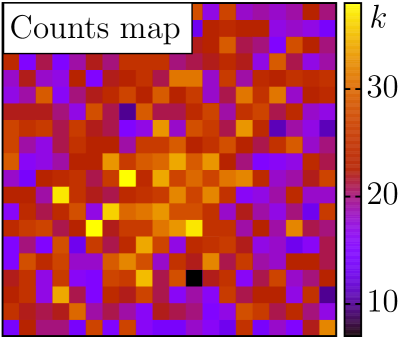
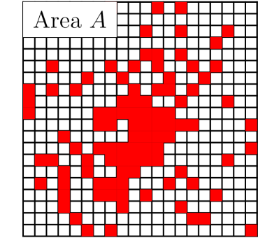
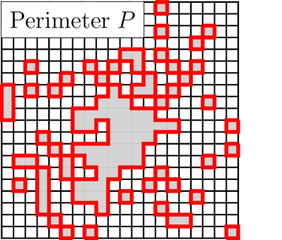
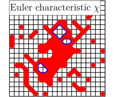
Figure 1: Structure quantification via Minkowski functionals. (a) Counts map, simulated Poisson-distributed random number of counts $k$. To characterize the morphology, the image is turned into a black-and-white image via thresholding — see (b); the three Minkowski functionals are then evaluated for the b/w image. (b) Area $A$. (c) Perimeter $P$. (d) Euler characteristic $\chi$.

A gray-scale image, here the counts map, is turned into a black-and-white (b/w) image (Mecke 1996). For each threshold value $\rho$, all pixels with counts $k\geq\rho$ are set to black, the others remain white — see Fig. 1. The structure of the image is then analyzed as a function of the threshold $\rho$.

The structure of each b/w image is quantified by the Minkowski functionals. In two dimensions there are three of them. They are proportional to well-known geometric quantities: the area $A$ of the black pixels, their perimeter $P$, and the Euler characteristic $\chi$, which is the integral of the Gaussian curvature. It is a topological constant; for closed domains it is given by the number of components minus the number of holes. Figure 1 visualizes how a counts map 1 is turned into a b/w image 1, which is then quantified by Minkowski functionals 1-1. The area as a function of the threshold contains the knowledge about the number of counts. However, it does not supply any information about their arrangement, for which additional information is provided by the perimeter and the Euler characteristic.

The Minkowski functionals are powerful shape measures. Because of their additivity and continuity, they are robust against noise and have short computation times. There are several linear time algorithms for calculating the area, perimeter, and Euler characteristic (e.g. Mantz et al. 2008; Schröder-Turk et al. 2010) and for $3\,\mathrm{D}$ data (e.g. Arns et al. 2010; Schröder-Turk et al. 2011, 2012).

Table 1: Look-up table for Minkowski functionals: the functional values of area $A$, perimeter $P$, and Euler characteristic $\chi$ are assigned to each 2x2 neighborhood of the image. The unit of length is the edge-length of a pixel. Similar data can be found in Mecke (1996) and Mantz et al. (2008).

Conf.		$A$	$P$	$\chi$	Conf.		$A$	$P$	$\chi$
1		0	0	0	9		1/4	1	1/4
2		1/4	1	1/4	10		1/2	2	-1/2
3		1/4	1	1/4	11		1/2	1	0
4		1/2	1	0	12		3/4	1	-1/4
5		1/4	1	1/4	13		1/2	1	0
6		1/2	1	0	14		3/4	1	-1/4
7		1/2	2	-1/2	15		3/4	1	-1/4
8		3/4	1	-1/4	16		1	0	0

The straightforward algorithm used here is based on Table 1. The image is decomposed into $2\times 2$ neighborhoods. The value of the Minkowski functionals is assigned to each of the 16 possible configurations. Because of their additivity, the sum of the local contributions yields their global value. The unit of length is defined as the edge-length of a single pixel, thus the area of a pixel is one. To avoid multiple countings when iterating over the whole image, only that part may contribute which is unique to a $2\times 2$ neighborhood, i.e., each quarter of the four pixels next to the center. For example, a single black pixel has area and Euler characteristic one and perimeter four. However, when iterating over the image, it will appear in four different 2x2 neighborhoods, namely configurations two, three, five, and nine. Thus, Table 1 assigns to each of them area and Euler characteristic one fourth and perimeter one. The white pixel in configuration 15 can be interpreted as part of a hole; it contributes negatively to the Euler characteristic. In configurations seven and ten in Table 1 the black pixels sharing only a vertex are chosen to be connected. If they were disconnected, the weights for the Euler characteristic would be positive. The choice is arbitrary, as long as the probability distribution for the Euler characteristic is calculated consistently. However, connecting them helps to distinguish a single cluster of black pixels from two domains distant from each other.

The choice of boundary conditions has a strong influence on the structure quantification and its efficiency (Stoyan et al. 1987). Throughout this work, closed boundary conditions are applied. This means all pixels outside the window of observation are set to white, thus all domains are closed. A discussion of the different impacts and drawbacks of various boundary conditions is beyond the scope of this paper and will follow in future publications.

Hadwiger’s completeness theorem ensures that the Minkowski functionals provide a robust and comprehensive morphology analysis, i.e., the Minkowski functionals form a complete basis of all valuations that are defined on unions of convex sets and are motion invariant, additive, and at least continuous on convex sets (Hadwiger 1957). To quantify anisotropy, they can be generalized to tensor valuations (e.g. Schneider & Weil 2008; Schröder-Turk et al. 2010, 2011).

3 Source detection

3.1 Global null hypothesis test

Structural deviations from the background morphology are to be detected. Therefore, the characteristic structure of a background measurement has to be known. Because the Minkowski functionals quantify the morphology, the probability distribution $\mathcal{P}$ of their functional value $X\in\{A,P,\chi\}$ for a counts map of a background measurement is needed. The first step is to choose a suitable background model.

In general, determining $\mathcal{P}(X)$ is the most complex task in the morphometric analysis. A reasonable model for background counts in VHE gamma-ray astronomy is the assumption of homogeneously and isotropically Poisson-distributed counts in each bin of a sky map with equal area bins. This is because most background events in ground-based VHE gamma-ray astronomy are caused by VHE hadrons. These hadrons loose their direction correlations in interstellar magnetic fields and arrive at the Earth as a uniform flux of VHE particles from every direction. For a real measurement the homogeneous and isotropic background will of course be distorted by detector effects and non-uniform exposure of the sky. As we show in section 4.1, the data can be corrected for these effects, i.e., the typical structure of a background measurement can be derived from the structure of a pure homogeneous and isotropic Poisson background.

The likelihood for the area $A$ of the black pixels is a suitable introductory example; the probability distribution for each threshold $\rho$ is given by the binomial distribution

$$\mathcal{P}(A) =\mathrm{Binom}(A,p_{\rho},N^{2})\,,$$

where $A$ is the number of black pixels, $N^{2}$ the number of pixels in an $N\times N$ sky map, and $p_{\rho}$ the probability that a pixel is black, i.e., there are more counts or their number is equal to the threshold $\rho$. Assuming a Poisson background with an expected number of counts per bin of $\lambda$, $p_{\rho}$ is given by

$$p_{\rho} =\sum_{i=\rho}^{\infty}{\frac{\lambda^{i}}{i!}e^{-\lambda}}\,.$$ (1)

The probability distributions $\mathcal{P}(A)$, $\mathcal{P}(P)$, and $\mathcal{P}(\chi)$ of the area, perimeter, and Euler characteristic, respectively, are plotted in Fig. 2 (a-c) as a function of the probability $p_{\rho}$ that a pixel is above the threshold $\rho$. For small $N$ these distributions can be found by evaluating all possible b/w images and inferring the distribution by counting equivalent pixel configurations.

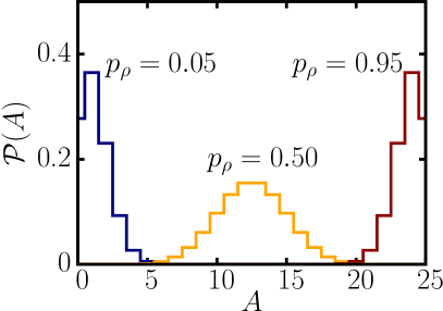
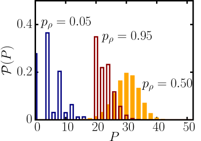
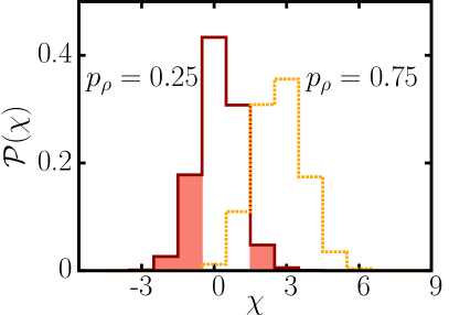
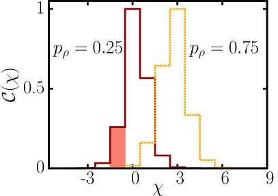
Figure 2: Structure of background noise for a $5\times 5$ bin field at different thresholds $\rho$ resulting in different probabilities $p_{\rho}=\sum_{i=\rho}^{\infty}{\lambda^{i}\,e^{-\lambda}/i!}$ for a black pixel. Probability distributions $\mathcal{P}$ of (a) area $A$; (b) perimeter $P$; (c) Euler characteristic $\chi$. (d) Compatibility $\mathcal{C}$ of Euler characteristic $\chi$, with $\mathcal{C}(\chi=-1)$ the sum of all probabilities $\mathcal{P}\leq\mathcal{P}(\chi=-1)$, which is visualized by the equally large colored regions beneath the graphs in (c) and (d) - mind the different scales.

Gamma-ray sources can be detected by looking for structures, which are very unlikely to be found if the hypothesis of a pure background measurement was true, i.e., assuming that there are only background events within the observation window. A probability measure that a given counts map with a structural value $X$ is compatible with this hypothesis may be defined as follows: The compatibility

$$\mathcal{C}(X) =\sum_{\mathcal{P}(X_{i})\leq\mathcal{P}(X)}\mathcal{P}(X_{i})$$ (2)

is the probability that a less likely structure appears. Figure 2 (d) shows the compatibility $C(\chi)$ for the Euler characteristic from Fig. 2 (c).

The compatibility is defined following the scheme given in Neyman & Pearson (1933) to construct a most efficient hypothesis test. The form used here may be derived from the general scheme given in the paper by setting the supremum of alternative hypotheses to $1$, i.e., imposing no constraints on alternative hypotheses. The hypothesis of a pure background measurement is rejected if the compatibility is lower than $0.6\cdot 10^{-6}$. This hypothesis criterion is adjusted to the commonly used $5\,\mathrm{\sigma}$ deviation; a normally distributed random variable deviates from the expected value by at least $5\,\mathrm{\sigma}$ with a probability of approximately $0.6\cdot 10^{-6}$.

Instead of dealing with tiny compatibilities, it is often more convenient to use the logarithm of this likelihood value or to define the deviation strength

$$\mathcal{D}:= -\log_{10}(\mathcal{C})\,.$$ (3)

The conversion between compatibility $\mathcal{C}$ and standard deviation $\sigma$ is given by $\mathcal{C}(\sigma)=\mathrm{erfc}\left(\sigma/\sqrt{2}\right)$, where $\mathrm{erfc}(x)=\frac{2}{\sqrt{\pi}}\int_{x}^{\infty}{\exp(-t^{2})\;\mathrm{d}t}$ is the error function.

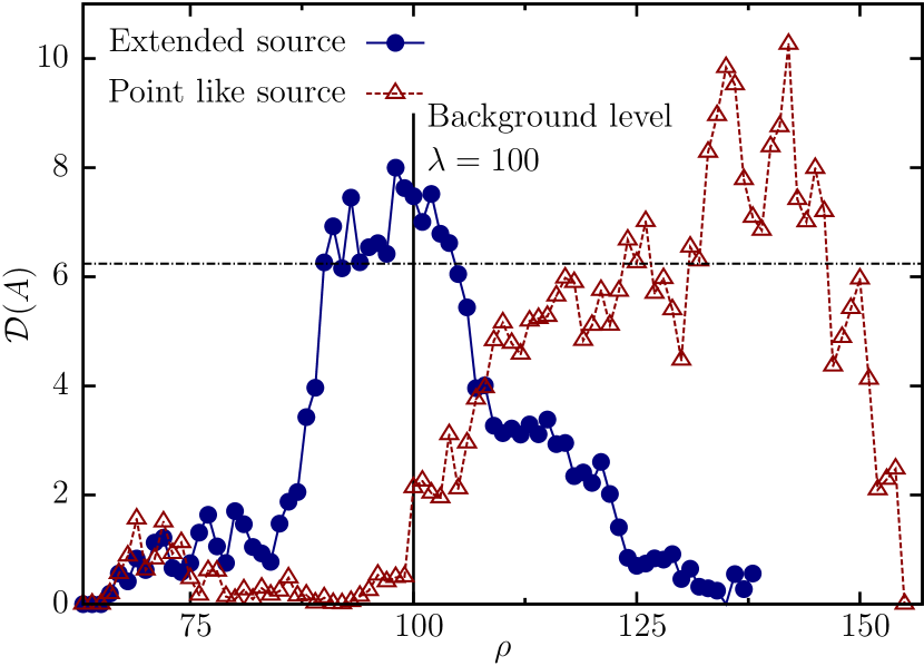
Figure 3: Deviation strength $\mathcal{D}(A)$ for structure quantification via area $A$ as a function of the threshold $\rho$ for an extended and for a point source of equal flux within an observation window of $100\times 100$ bins.

Figure 3 depicts a structure analysis of both a rather extended and of a more point-like source, investigating simulated data of Poisson-distributed random number of counts. The deviation strength $\mathcal{D}$ is plotted over the threshold $\rho$. Because there are thresholds for both sources for which the deviation strength is greater than $6.2$, the null hypothesis of a pure background measurement can be rejected in either case. The results differ for the two sources, but their total flux is equal, and reveals basic information about the extension of the sources. The point source cannot be detected at thresholds near the background level $\lambda$ and is only apparent for high thresholds, i.e., only bins with high counts contribute to the detection. For the extended source only counts in the order of the magnitude of the background fluctuations are present in the sky map. However, as the number of bins with slightly increased counts exceeds the typical background predictions, the hypothesis is nevertheless rejected.

3.2 Local Minkowski sky maps

So far, it is possible to scan the entire field of view (FoV) of an observation for additional structures w.r.t. the expected background. To localize the deviations and thus locate gamma-ray sources and gain insight into their extension and morphology, more information is needed. Owing to their motion invariance, the scalar Minkowski functionals cannot be used directly to localize structures.

Instead of analyzing the entire FoV with the methods introduced so far, a small sliding window may be used. This window can be moved across the FoV to study the local structure of the sky map in the sliding window. With this approach one can construct Minkowski sky maps from the counts maps that are just as useful as significance maps constructed using the approach from Li & Ma (1983), but which provide the additional sensitivity from the structure information used to determine the deviation strength.

Since the maximum deviation strength is assigned to a pixel, a trial factor must be added to the result to avoid overestimating the significance of the found deviations (Göring 2012). Each of the different b/w images for different thresholds $\rho$ contributes a trial to the search for structure deviations, and as the number of trials increases, the probability to find a significant random fluctuation increases as well. Assuming one looked for measurements with a compatibility lower than $\alpha$, the probability to find such a deviation in one image is $\alpha$. The probability to find no such deviation in $t$ independent images is $(1-\alpha)^{t}$ and the probability to find at least one such deviation in the image set is $1-(1-\alpha)^{t}$. Thus, the significance after $t$ independent trials is linked to the pre-trial significance $\alpha$ via

$$\alpha_{t}=1-(1-\alpha)^{t}=t\alpha+\mathcal{O}(\alpha^{2})\,.$$ (4)

Accordingly, for $\alpha\ll 1$ the influence of $t$ independent trials may be approximated by the so-called trial factor, i.e., by multiplying $\alpha$ with $t$. For the corresponding deviation strength $\mathcal{D}_{t}$ this results in an offset of $\log_{10}(t)$ compared with the pre-trial deviation strength $\mathcal{D}$, i.e., $\forall\mathcal{D}\gg 0:\mathcal{D}_{t}\approx\mathcal{D}-\log_{10}(t)$.

Obviously, the different b/w images resulting from thresholding are not statistically independent, because they originate from the same intensity profile. If the structure of a b/w image at a certain threshold can be interpolated from the structures of the b/w images of the next higher and lower thresholds, it does not contribute a separate trial to the search for deviations from the null hypothesis. Therefore, if $t$ is set to the number of threshold steps, Eq. (4) will yield a conservative estimate of the post-trial significance.

A rough estimate of the systematic error on the deviation strength $\mathcal{D}$ introduced by ignoring the influence of trial factors is given by $2\log_{10}(N)$. This estimate is based on the fact that the number of different b/w images after thresholding is equal to the number of different gray levels in the original gray-scale image that represents the gamma-ray counts map. There are at most $N^{2}$ different gray levels in an image of $N\times N$ pixels and therefore at most $N^{2}$ different trials may contribute to the search for structure deviations; from $t\leq N^{2}$ follows

$$\mathcal{D}_{t}\approx\mathcal{D}-\log_{10}(t)\geq\mathcal{D}-2\log_{10}(N)\,.$$ (5)

Therefore, $\mathcal{D}-2\log_{10}(N)$ may be used to compute a conservative estimate of the post-trial deviation strength; for the preceding discussion see Göring (2012).

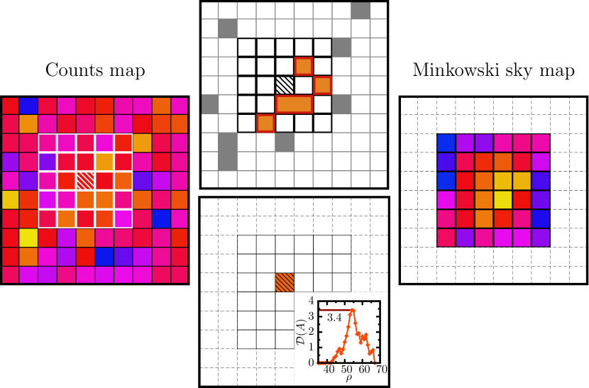
Figure 4: Computation of a Minkowski sky map. LEFT: a given counts map. MIDDLE: for each pixel the local structure within the sliding window is characterized (top) and the maximum deviation strength for all thresholds is assigned to it in the Minkowski sky map (bottom). RIGHT: iterating through all pixels provides the Minkowski sky map.

Figure 4 depicts the concept of a Minkowski sky map. For each of the inner pixels of the counts map the local structure is to be characterized (depicted on the left). Therefore, the Minkowski functionals of a sliding window with $N\times N$ pixels are evaluated (illustrated in the top picture in the middle of Fig. 4). The maximum deviation strength for all thresholds $\rho$ is assigned to the pixel at the center of the sliding window (plotted in the bottom picture in the middle). Iterating over all inner pixels for which the sliding window is completely within the counts map provides the Minkowski sky map.

The information content and intuitive interpretation of such Minkowski sky maps can be enhanced by adding a sign to the deviation strength of the different pixels. By choosing the sign to be negative if $A<N^{2}p$, i.e., if there are fewer black pixels than expected, and positive otherwise, the sign of a pixel shows if the local deviation is caused by an overestimation of the background or by additional flux from potential gamma-ray sources. Minkowski sky maps detect local structural deviations and depict them in an illustrative and quantitative image, depicting the lack of trust in the hypothesis that there are only background fluctuations.

Although the null hypothesis is tested locally, the background assumption is a global null hypothesis, i.e., the expected number of counts per bin $\lambda$ is chosen globally. If $\lambda$ is chosen locally for every sliding window, structures larger than the sliding window may result in an increased $\lambda$ and in no deviation at all if the local structure is homogeneous and isotropic within the sliding window.

3.3 Simulated data

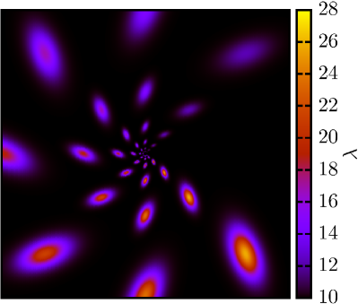
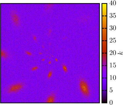
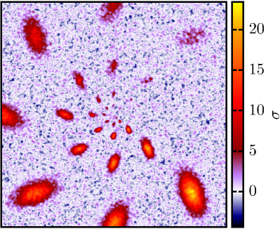
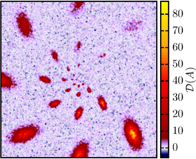
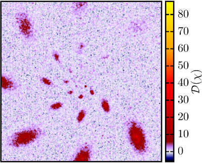
Figure 5: Structure analysis of simulated sky maps. 5 Given intensity profile. 5 Simulated counts map. 5 Significance map, evaluated with standard techniques, weighting the count excess. 5 Minkowski sky map; the structure is characterized with the area $A$, 5 the perimeter $P$, and 5 the Euler characteristic $\chi$.

It is now possible to detect, localize, and study the shape of gamma-ray sources using the morphometric analysis with Minkowski sky maps, introduced in the previous section. Figure 5 depicts an analysis of exemplary simulated data. Figure (a) shows the given intensity profile of the test pattern sources, the expected number of counts per bin caused by the chosen sources. The test pattern consists of Gaussian-shaped extended sources with a ratio of the semi-major axes of $2$. The peak intensities of the sources along a central ray from the image center are equal. The sizes of sources with the same distance from the center are equal and the peak intensities are increasing in counter-clockwise direction. Plot (b) is the simulated counts map analyzed in (c-f). In figure (c) the standard analysis technique of Li & Ma (1983) as used by the H.E.S.S. experiment (cf. F. Aharonian et al. 2006) is applied to the counts map (b) for comparison. Figures (d-f) are the Minkowski sky maps with a sliding window size $5\times 5$; the structure is quantified by either the area $A$, the perimeter $P$, or the Euler characteristic $\chi$. The same $5\times 5$ window is used as on-region for the significance determination using Li & Ma (1983).

The first apparent result drawn from Fig. 5 is that the single functionals and the standard analysis are similarly sensitive to sources; area, perimeter, and Euler characteristic are comparably competitive in finding gamma-ray signals.

4 H.E.S.S. data

4.1 Detector acceptance correction

An analysis of real data must always take into account the detector acceptance. After modeling the camera acceptance, the effect must be corrected for to regain an isotropic and homogeneous structure for background measurements. For each bin $i$ only a fraction $f_{i}$ of the signals are expected to be detected. If each bin is simply weighted with $1/f_{i}$, fractional photon counts will occur that destroy the Poisson structure of the sky map.

The null hypothesis, that is, that for an ideal camera acceptance there is only background noise with intensity $\lambda$, allows an acceptance correction, which preserves the Poisson structure. Because only the fraction $f_{i}$ of the events in bin $i$ are detected, the actual background intensity $\lambda_{i}=f_{i}\cdot\lambda$ varies with each bin. Following the null hypothesis, that the number of counts is a Poisson-distributed random variable with mean $\lambda_{i}$, the original random process with mean $\lambda$ can be regained if a new Poisson-distributed random variable with mean $\lambda_{i}^{+}=(1-f_{i})\cdot\lambda$ is added.

In the center of the field of view, where $f_{i}\approx 1$, the number of counts remains effectively unchanged. For $f_{i}\ll 1$ the additionally created pseudo-photon counts may cover features, but they never introduce additional structural deviations from the homogeneous isotropic Poisson field because they fulfill the given null hypothesis by construction. Covering regions of low acceptance with a layer of pseudo-events corresponds to the fact that the instrument is less sensitive to signals in these regions than in regions with high acceptance – see also Göring (2008), Klatt (2010), and Göring (2012).

4.2 H.E.S.S. source

With the methods discussed so far, we can analyze experimental data of ground-based VHE gamma-ray telescopes such as the H.E.S.S. experiment. Because the morphometric analysis is targeted at extended structures, RX J$1713.7\!-\!3946$ was chosen for an exemplary analysis. This source has one of the largest angular diameters of the sources seen with H.E.S.S. and its morphology has already been studied in detail and is well known (Aharonian et al. 2006a), which makes it a suitable benchmark for more detailed analyses.

The data set used for analysis corresponds to the data used in Aharonian et al. (2006a), but instead of the Hillas-based event reconstruction discussed there, the advanced event reconstruction based on a likelihood-model fit presented in de Naurois & Rolland (2009) was used to compute the list of reconstructed events from the recorded camera images. These reconstructed events were used to fill the binned counts map, which is the main input of the morphometric analysis.

The second input needed is an acceptance map describing the spatial sensitivity of the given observations, which is used to perform the acceptance correction discussed above. This map was created using standard H.E.S.S. analysis tools. In particular, the so-called $2\,\mathrm{D}$ acceptance model discussed in de Naurois (2012) was used. The overall background level $\lambda$ was determined from the counts map by excluding all regions containing known sources of VHE gamma-rays and computing the mean of the counts in the remaining bins normalized by the corresponding acceptance.

Figure 6 shows the resulting Minkowski sky maps of a morphometric analysis based on the area $A$, the perimeter $P$, and the Euler characteristic $\chi$. The underlying counts and acceptance maps used for this analysis were created using square bins of $0.02\,\mathrm{\degree}$ width. The resulting sky maps clearly show RX J$1713.7\!-\!3946$ and agree well with the results of the standard H.E.S.S. analysis given in Aharonian et al. (2006a). This demonstrates that an analysis based on the structure of the measured counts map is indeed possible and provides results comparable with those of well-established tools.

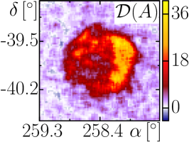
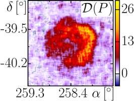
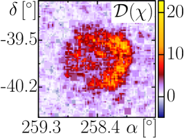
Figure 6: Minkowski sky maps of RX J$1713.7\!-\!3946$. The morphometric analysis is based on (a) area $A$, (b) perimeter $P$, and (c) Euler characteristic $\chi$.

5 Conclusion and outlook

The introduced morphometric analysis provides a novel approach to data analysis in VHE gamma-ray astronomy. In contrast to the commonly applied hypothesis test by Li & Ma (1983) to detect a significant excess of gamma-ray counts on top of the expected background, it allows one to incorporate additional morphometric information into the analysis of gamma-ray counts maps. Still, the underlying model depends only on $\lambda$, the expected background level of a given measurement, and there is no need for a priori modeling of potential sources, as opposed to an analysis based on a likelihood fit of a comprehensive model to the data, as commonly used in satellite-based gamma-ray experiments, for instance, Fermi/LAT (Atwood et al. 2009). Klatt et al. (2012) provided a short introduction to the shape analysis of counts maps.

The morphometric analysis is based on the characterization of the typical structure of a pure homogeneously and isotropically Poisson-distributed background counts map. This typical structure is determined using the Minkowski functionals — morphometric valuations from integral geometry. Significant deviations from the typical background structure in measured gamma-ray counts maps can be used to detect gamma-ray sources in the same way as significant excess counts are used in analyses based on Li & Ma (1983).

With our basic ideas, it is possible today to qualitatively reproduce analysis results based on well-established tool chains. To quantify the agreement of the different analysis techniques and potential sensitivity gains of the new morphometric approach, more in-depth studies are required. Still, there are strong indications that the presented methods will lead to a significant sensitivity gain in the foreseeable future. Current proof-of-concept studies show an impressive performance and a similar sensitivity of the three Minkowski functionals to deviations from the background structure. Combining the different functionals to refine the background characterization may well lead to a significant sensitivity boost. Furthermore, the Minkowski functionals can be generalized to tensor-valued valuations. These Minkowski tensors quantify additional morphometric information such as isotropy and homogeneity and thus provide a comprehensive view of the available morphological information. Incorporating this additional information may increase the sensitivity of the morphometric analysis even more. The inherent potential of our methods provides some exciting perspectives for data analysis in VHE gamma-ray astronomy.