Duality and Higher Temperature Phases of Large Chern-Simons Matter Theories on
Abstract:
It has been recently demonstrated that the thermal partition function of any large Chern-Simons gauge theories on , coupled to fundamental matter, reduces to a capped unitary matrix model. The matrix models corresponding to several specific matter Chern-Simons theories at temperature were determined in [1]. The large saddle point equations for these theories were determined in the same paper, and were solved in the low temperature phase. In this paper we find exact solutions for these saddle point equations in three other phases of these theories and thereby explicitly determine the free energy of the corresponding theories at all values of . As anticipated on general grounds in [1], our results are in perfect agreement with conjectured level rank type bosonization dualities between pairs of such theories.
1 Introduction
Recently, three dimensional field theories have become fascinating in the context of AdS/CFT (or dS/CFT) correspondences which do not necessarily rely on supersymmetry [2]. It has been recently conjectured that level Chern-Simons theories with matter in the fundamental/bifundamental representations admit a dual description governed by parity violating Vasiliev’s higher spin equations [3, 4] (see [5] for more detail and references) at finite values of the ’t Hooft coupling [6, 7].
Sometimes, analysis of boundary field theories can be applied to study bulk gravity theories through the AdS/CFT correspondence when the direct analysis of the gravity theory is difficult. For example, it is known that the AdS/CFT correspondence maps deconfinement transitions of large gauge theories on spheres to gravitational phase transitions involving black hole nucleation [8]. This observation has motivated the intensive study of the phase structures as well as the deconfinement phase transitions of large p+1 dimensional Yang Mills theories (coupled to adjoint and fundamental matter) on . Now, we can expect similar application of the Chern-Simons matter theories to know the phase structures of parity violating Vasiliev’s higher spin gravity theories.
From this motivation, in [1], the finite temperature phase structure of renormalized level U() Chern-Simons (CS) theories coupled to a finite number of fundamental fields on in the t’ Hooft limit , with fixed were studied. The phase structure was studied by using a simple toy large Gross-Witten-Wadia (GWW) matrix integral, and it turned out that there is a rich phase structure caused by the summation over the flux sectors in the Chern-Simons theory. In particular, the eigenvalues must be discretized and the eigenvalue density function must be saturated from upper bound . This saturation was first suggested by [9]. This discretization generates the new phases so-called the “upper gap phase” and the “two gap phase”, which are absent in Yang-Mills theories. 111 The same upper bound for the density function appears in two dimensional Yang-Mills theory (), in which case the situation becomes similar due to the fact that there are no propagating degrees of freedom for the gauge field. A phase transition relevant to this upper bound was studied in 2d (q-deformed) Yang-Mills theory on [10, 11, 12, 13], which we will see from Chern-Simons theory. The level-rank duality has also been confirmed in the GWW toy model in [1] (see [14, 15] for a relatively recent discussion of level-rank duality and references to earlier work), but the phase structures of the actual Chern-Simons matter theories have not been worked out. Moreover, we have not had the perfect analytic proof of the duality, even in the GWW model.
In this paper we will work out the study of the phase structure of several Chern-Simons matter theories: (1) the CS theory minimally coupled to the fundamental fermion [6], (2) the CS theory coupled to massless critical bosons [16, 17], and (3) the supersymmetric CS theory with a single fundamental chiral multiplet [18, 19] (SUSY CS matter theory). We will also provide the perfect analytic proof of the level-rank duality (Giveon-Kutasov type duality) on the between the regular fermion theory and the critical boson theory. Moreover we will prove the level-rank self-duality in both the SUSY CS matter theory and the GWW matrix integration as well. We will also supply several useful formulae which can be used for any analysis related to the duality in general CS matter theories on .
1.1 Outline of this paper
The rest of this paper is organized as follows: In section 2 we will review the Landau-Ginzburg description of the partition function of Chern-Simons theories coupled to fundamental matters as a preliminary, and supply techniques to evaluate eigenvalue densities as well as partition functions by using complex line integration in the complex plane. In section 3, we will elaborate the phase structure of the regular fermion theory and the critical boson theory, confirming that the level-rank duality between them is in agreement. In section 4, we will study the phase structure of the supersymmetric CS matter theory and examine the Giveon-Kutasov type duality. We will confirm the self-duality of the theory. In section 5, we will give the analytic proof of the level-rank self-duality in the two gap phase of the GWW toy model. Section 6 is devoted to the summary and discussion.
The content of the appendix is as follows: We put several definitions of the cut regions and cut functions in appendix A. We give the proof of important formulae used in the proof of the duality and others in appendix B. In appendix C, we provide the detailed analysis of the large behavior of the eigenvalue density functions. In appendix C, we also prove that the eigenvalue distributions at converge to the universal distribution (16).
2 Preliminaries
2.1 High temperature effective action of the Chern-Simons-fundamental matter theory on
We will consider the level fundamental matter Chern-Simons theories in the ’t Hooft large limit, with222 We use the dimensional reduction regulation scheme throughout this paper. In this case , where is the level of the Chern-Simons theory regulated by including an infinitesimal Yang Mills term in the action, and is the level of the theory regulated in the dimensional reduction scheme [20, 21]. For this reason this class of Chern-Simons theories may be well-defined only in the range . Hereafter we assume that the ’t Hooft coupling is always positive for simplicity. Our results are easily generalized to the case where is negative by taking the absolute value of it.
| (1) |
where and are held fixed in the large limit. These theories have recently been studied intensively at finite [6, 16, 22, 23, 24, 7, 17, 25, 26, 27, 28, 9], and thermal partition functions of these theories are studied in [29, 6, 7].
We will consider the partition function of these theories
| (2) |
where denotes the integration measure of matter fields. To calculate it, we will integrate the matter fields first, and obtain the effective action which depends on the gauge fields. According to the study in [1], the partition function is given as
| (3) |
where is a function of the two dimensional holonomy fields around the thermal circle . Here of indicates a point on the , and its eigenvalue is where is the index of matrix. The effective action would be obtained by summing up all vacuum graphs which involve at least one matter field. The graphs which do not involve any matter fields are not summed yet, but they are summed at the stage of the path integration in (3).
To calculate (3), it is useful to observe that is ultralocal in large as well as in high temperature. The would be expanded as a series of local operators,
| (4) |
Note that the scaling (1) converts higher temperature expansion (4) into expansion in inverse power of . Here the first term is leading and the second term is and terms are further suppressed at large . 333Every term in the effective action (4) is of order at fixed , as the action is generated by integrating out fundamental fields. Then at large , the effective action is simplified to be the leading term
| (5) |
This (5) is originally suggested in [9], which is a consequence of the entire effect of matter loops on gauge dynamics at temperature and at leading order in . By (5), the partition function would be given by
| (6) |
where
| (7) |
is the expectation value of in the pure Chern-Simons theory at level . Since the Chern-Simons theory is topological, expectation values become independent of , then the dependence is removed in the step from the second line to the third line of (6). Here is the volume of .
2.2 Path integration to obtain the partition function, deconfinement phase transition and further phase transition caused by flux
We can perform the calculation of (6) in the same manner as [30]. You can see the details of how to compute the path integration in [1]. Keeping the effective potential term intact, we achieve the following value
| (8) |
where are constant units of flux in the factors. As we can see in the last line, the summation over flux in constrains to take discrete values
| (9) |
Then the partition function would be
| (10) |
where the summation over is restricted so that no two are allowed to be equal.
2.3 Eigenvalue density
We will estimate (10) in the ’t Hooft limit, . The summation over the eigenvalue (10) in the limit is dominated by the saddle point configuration of the eigenvalues at large . The saddle points minimize the following potential
| (11) |
where . The saddle points are obtained by solutions of the following equation
| (12) |
In terms of eigenvalue density function , the equation would be represented by
| (13) |
where .
We can see that this saddle point equation problem is very similar to the Gross-Witten-Wadia (GWW) problem [31, 32, 33] in the Yang-Mills theory on . In a usual GWW problem in Yang-Mills theories, a thermal partition function obtained after integrating out all massive modes is given by the integration over the single unitary matrix as
| (14) |
and there is a competition between potential that tends to clump eigenvalues, and the measure factor (Vandermonde determinant) which tends to repel them. 444 The effective potential was computed in free gauge theories [34, 35]; it has also been evaluated at higher orders in perturbation theory in special examples [36, 37, 38, 39]. At least in perturbation theory [35] and perhaps beyond [40, 41], the potential is an analytic function of . At low temperature with small , the repulsive force by the measure factor is stronger. Then the eigenvalue density would have support everywhere on . But on the other hand, in the high enough temperature, the attracting force caused by the potential becomes stronger than the repulsive force, and the eigenvalue will be clumped. Then in the high temperature the eigenvalue distribution has support only on a finite arc, there would be a domain of eigenvalues so-called ”lower gap” such that , and phase transition would occur. At extremely high temperature , the eigenvalue density function would be clumped to be a delta function .
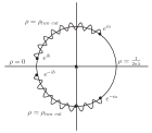
Also in the current Chern-Simons case (10), such a competition between and measure term exists. But in this case, unlike the usual Yang-Mills case (14), there is a constraint on the eigenvalue (9). (9) saturates the eigenvalue density from above as
| (15) |
while the eigenvalue density in the Yang-Mills theory is not bounded from above (is bounded only from below). Saddle points of (14) do not always obey the inequality (15), then the Yang-Mills solutions violating (15) will not be the solution of the Chern-Simons saddle point equations (13) and (10). Instead, the current Chern-Simons theory admits new classes of solutions saturating the upper bound of the inequality over several arcs along the unit circle. Hence in this Chern-Simons case, there can exist not only the ”lower gaps” but also the ”upper gaps”, which are arcs over which the upper bound of (15) are saturated.
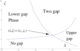
Hence the phase structures of the current Chern-Simons theories (10) would be different from the one of usual Yang-Mills theory (14). In a usual Yang-Mills theory case, there are only two phases, ”no gap phase” and ”lower gap phase”. In the no gap phase, the eigenvalue has support everywhere on the unit circle in the complex plane, on the other hand in the lower gap phase, the eigenvalue has support only on a finite arcs. On the other hand, in the current Chern-Simons case, due to the existence of upper bound (15), not only the no gap and lower gap phases, but also ”upper gap” and ”two gap” phases exist. In the upper gap phase, there is one upper gap where the upper bound of (15) is saturated, and the eigenvalue density has support everywhere on the unit circle. In the two gap phase, there is one upper gap as well as one lower gap where the eigenvalue density vanishes.
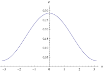
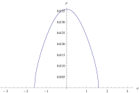
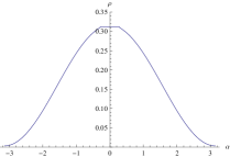
In the Chern-Simons case, the eigenvalue distribution is in the no gap phase in the low temperature, and if we increase the temperature, eigenvalue density starts to clump to , and then we can expect lower gaps or upper gaps will show up. In the small ’t Hooft coupling region , since the upper bound in (15) is large enough, lower gaps will show up before the maximum of the eigenvalue density function reaches the upper bound. Then it transits to lower gap phase first. As we increase the temperature further, the maximum of the eigenvalue density eventually reaches the upper bound and it transits to the two gap phase. On the other hand, at large with , the upper bound in (15) is small, then the maximum of the eigenvalue reaches the upper bound before the lower gap shows up. Then in the large region, it transits to upper gap phase first. If we increase the temperature further, since the eigenvalue density keeps clumping, lower gaps will show up and it transits to two gap phase. In the large limit, the eigenvalue density will have a universal configuration
| (16) |
which is the nearest thing to a function permitted by the effective Fermi statistics of the eigenvalues . This is in perfect agreement with the results of [9] in which they used the Hamiltonian methods [42].
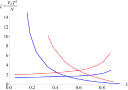
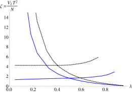
For your reference, you can see the graph of the eigenvalue density function in each phase listed in Figs.1 1. You can also see the phase diagrams of Chern-Simons matter theories in Figs.2 4 and 6.

2.4 How to calculate the eigenvalue density in lower gap, upper gap and two gap phases
In this subsection we will review how to obtain the eigenvalue density in the lower gap, the upper gap and the two gap phases. To calculate the eigenvalue density, we will decompose the eigenvalue density to . By substituting it into the saddle point equation we can rewrite the saddle point equation as
| (17) |
Here is nonzero in the compliment of both upper gaps and lower gaps. Starting from this, we turn to the complex variables
Note that
Here (17) will be rewritten in terms of these variables as
| (18) |
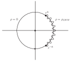
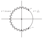
where the integrals in (18) run counterclockwise over the unit circle in the complex plane. Suppose that the solution to this equation, , has support on connected arcs on the unit circle in the complex plane. We denote the beginning and endpoints of these arcs by and (). These are the endpoints of lower gaps or upper gaps as well. Our convention is that the points , , , , sequentially follow each other counterclockwise on the unit circle. We refer to the arcs as ‘cuts’. The arcs (as also ) are referred to as gaps. By definition, has support only along the cuts on the unit circle.
We use the (as yet unknown) function to define an analytic function on the complex plane
| (19) |
where the integral is taken counterclockwise along the cuts, of the unit circle in the complex plane. It is easy to see that the analytic function is discontinuous along these cuts. Let denote the limit of as it approaches a cut from , and let denote the limit of as it approaches a cut from . Then 555We use analogous notation for other analytic functions below. Let denote a complex number of unit norm. The symbol will denote the limit of as from above (i.e. from ), while is the limit of the same function as from below (i.e. from ). Note that along a cut .
| (20) |
and
| (21) |
(the first equality is the definition of the principal value, while the second equality follows using (18)). Moreover it follows immediately from (18) and (19) that
| (22) |
We are now posed with the problem of determining given its principal value along a cut. To determine the , we introduce following ”cut function” as
| (23) |
We define to have cuts precisely on the arcs on the unit circle that extend from to . This definition fixes the function up to an overall sign. This sign will cancel out in our solution for below, and so is uninteresting. For future use we note that when ,
| (24) |
We use the function to define a new function, , via the equation
Using the fact that along the cut, (21) turns into
| (25) |
Here we assume that is holomorphic except in the cut region. From (22) and (23), at large so that
| (26) |
where the contour runs counterclockwise over a very large circle at infinity. Since is holomorphic except on the cut, by the Cauchy’s theorem,
| (27) |
The contour are the loops enclosing each of the cuts , but not the point . Then from (25),
| (28) |
In the equation above, is a variable on the complex plane while is a variable on the unit circle of the complex plane. The integration region runs counterclockwise along cuts on the unit circle (This is not loop !), integration region for each cut is from to . The third equality uses together with the assumption that has no singularities on the cuts.
Now by applying the Cauchy’s theorem for the integrand again, we will obtain the following
| (29) |
The last term is the sum of the residues of . Here we have assumed that is a meromorphic function of .
Based on in (29), and from , combining with , we can obtain the eigenvalue density . From next section, we will obtain the phase structure of the regular fermion theory, the critical boson theory and the supersymmetric CS matter theory by using the techniques supplied by this subsection.
3 Higher temperature phases of the regular fermion theory and critical boson theory and the duality
3.1 Regular fermion theory
In this subsection we study the level Chern-Simons theory coupled to massless fundamental fermions. The Lagrangian of the theory is presented in equation (2.1) of [6]. From the equation (3.5) of [1], effective potential is obtained as
| (30) |
where determines the thermal mass of the fermions.666 is the thermal mass of the fundamental fermions. More precisely, the fermionic self energy is given by , where (31) The value of is obtained by extremizing w.r.t at fixed , , i.e. obeys the equation
| (32) |
The general form of the free energy of the regular fermion theory on is given as
| (33) |
To obtain the free energy in each phase, we only have to evaluate the eigenvalue density and in each phase and just substitute into (33). Note that can be determined if the eigenvalue density is determined. So obtaining the eigenvalue density in each phase is equivalent to obtaining the free energy in each phase.
For later use, we will give the form of here. We obtain from (30) as
| (34) |
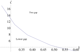
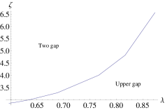
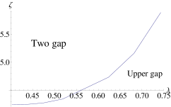
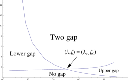
The phase structure of this theory is depicted in Fig. 2, as obtained in following subsubsections.
3.1.1 Lower gap phase
To obtain the eigenvalue density in the lower gap phase, we will employ the cut region and the cut function described in appendix A.1. The function as well as in the lower gap phase are obtained by using (29) with substituting . in (29) is identical to as
| (35) |
because . By substituting the above into (29), we immediately obtain as well as as,
| (36) |
3.1.2 Upper gap phase
Next we will search for a solution with no lower gap and one upper gap. The domain of cut and the cut function in this upper gap phase are defined in appendix A.2. To obtain the eigenvalue density based on (29), we will take at the upper gap region . Then by using (29) with (34), we obtain as well as as
| (39) |
where runs counterclockwise over upper gap region, and runs counterclockwise over unit circle.
From (39), and by taking at the cut region with , we can obtain the eigenvalue density function as
| (40) |
In the region , . To derive (40), we have used a formula
| (41) |
where the is located at the cut region. This is proved in appendix B.1.2. By substituting the eigenvalue density (40) into (32) and (33), we can obtain as well as the free energy in the upper gap phase of the regular fermion theory.
3.1.3 Two gap phase
Now we will search for a solution with one lower gap and one upper gap. The details of our two cuts and the cut function are described in appendix A.3.
The function as well as are obtained by using (29),
| (44) |
From , we obtain the following two conditions,
| (45) |
| (46) |
By using (45), (46) and (32), are determined as functions of as .
From (44) and by taking at the cuts , we obtain the eigenvalue density as
| (47) |
in , and in . During the calculation of (47), we have used (45) also. Here has the same functional form as the eigenvalue density in the GWW type matrix integration (7.6) in [1]. can be regarded as an additional term depending on the detail of the theory. By substituing the eigenvalue density (47) into (32) and (33), we can obtain as well as the free energy in the two gap phase. and can be represented by the complex line integral by taking as
| (48) |
These are useful to discuss the level-rank duality later.
The combination of (45), (46), (32) and (47) provides a complete set of solutions in the two gap phase.
At the large limit, as we proved in appendix C.1.1, the eigenvalue density approaches the universal distribution (16) because remains as a finite positive quantity at the limit. In the limit, , and the eigenvalue density behave as
| (49) |
At appendix C.2.1, we have demonstrated the above behavior (49). As we can see in the appendix, the eigenvalue density function is dominated by at the large limit. The form of the eigenvalue density approaches function which is the same form as (7.11) in [1] which is the large limit of the one of the GWW model. We can also see that the range of the domain of the cut is smaller than the one in the GWW type matrix integration at the same value of .
3.1.4 Phase transition points
Phase transition points between no gap and lower gap
Let us consider the behavior of the lower gap solutions (37) and (38) at the point which would correspond to the phase transition points from the lower gap to the no gap phase. If we substitute into (38), it becomes
| (50) |
This is exactly same as the condition for the phase transition from the no gap to the lower gap discussed in [1], which is obtained by substituting into the third line of (6.33) and by requiring . Based on this, if we substitute into (37), we can see
| (51) |
In the last step we have used (50), the Taylor expansion and
| (52) |
The last line of (51) is exactly same as the eigenvalue density function in the no gap phase described in the third line of Eq. (6.33) in [1]. So, at the phase transition points, the lower gap solutions are smoothly connected to the no gap phase solutions.
Phase transition points between no gap and upper gap
Let us consider the behavior of (40) and (42) at which would correspond to the phase transition points from the upper gap to the no gap phase. If we substitute into (42), it becomes
| (53) |
This is exactly same as the condition for the phase transition from the no gap to the upper gap phase discussed in [1], which is obtained by substituting into the third line of (6.33) and by requiring .
Based on this, if we substitute in (40), we can see
| (54) |
In the last step we have used (53), the Taylor expansion and the formula (52). The last line of (54) is exactly same as the eigenvalue density function in the no gap phase, described in the third line of Eq. (6.33) in [1]. So the upper gap solutions are smoothly connected to the ones in the no gap phase at the phase transition points.
Phase transition from the lower gap to the two gap
In the lower gap phase at fixed , the phase transition from the lower gap phase to the two gap phase will occur when the maximum of the eigenvalue density reaches . The condition would be represented as
| (55) |
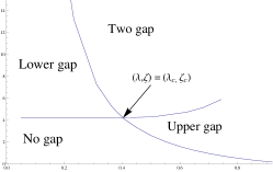
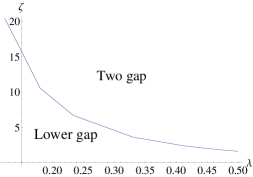
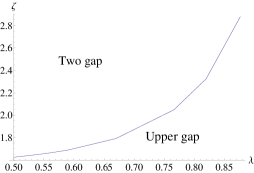
The combination of (55), (32) and (38) provides the phase transition points from the lower gap to the two gap. By numerical calculations based on (55), (32) and (38), we obtain the phase transition points plotted in Fig. 3.
Let us see the phase transition points from the standpoint of the two gap phase. If we substitute into (45), it becomes the same as (55), which is the condition for the phase transition points. If we set at (46), it becomes the same as (38). Let us check whether eigenvalue density in the two gap phase (47) becomes the one in the lower gap phase (37) in limit. By using (55), we can replace of (47) by
| (56) |
Then by summing up with , (47) at becomes (37). So we can see that solutions of two gap phase are smoothly connected to solutions of the lower gap phase at the phase transition point.
Phase transition from the upper gap to the two gap
In the upper gap phase, if the minimum of the eigenvalue density reaches to the phase transition from the upper gap phase to the two gap phase will occur. The condition would be represented as
| (57) |
The combination of (57), (42) and (32) provides the phase transition points from the upper gap to the two gap. By numerical calculations based on (57), (42) and (32), we have obtained the phase transition points plotted in Fig. 3.
Let us see the phase transition points from the standpoint of the two gap phase. If we substitute into (45), it becomes (57). By using the relationship (57), (46) at is reduced to (42). Let us check that the eigenvalue density in the two gap phase (47) at is smoothly connected to the one in the upper gap phase (40). To confirm it, first we apply the following formula
| (58) |
and then by using (57) we can rewrite as
| (59) |
Then by summing up with , we can see that (47) at becomes (40). So we can see that solutions of two gap phase are smoothly connected to solutions of the upper gap phase.
Quadruple phase transition point in the regular fermion theory
There is the quadruple phase transition point
| (60) |
at which the no gap, the lower gap, the upper gap and the two gap phase coexist. Let us check whether (60) is the quadruple phase transition point or not. Note that (50) is the condition for the phase transition from the no gap to the lower gap phase. Eq. (53) is the condition for the phase transition between the no gap and the upper gap, (55) is the one between the lower gap and the two gap, and (57) is the one between the upper gap and the two gap. So if (60) satisfies these four equations simultaneously, it would be the quadruple phase transition point. If we substitute into (55) it becomes
| (61) |
If we substitute into (57), it also becomes the same equation as (61). We can also see that if both (50) and (53) are simultaneously satisfied, (61) is also automatically satisfied. So if there is a point satisfying (61), the point becomes the quadruple phase transition point. By the study in [1], we already know that only the point (60) simultaneously satisfies both conditions (50) and (53). Hence (60) satisfies (61). So (60) becomes the quadruple phase transition point in the regular fermion theory. Then due to the existence of the quadruple point, the phase structure of the regular fermion theory becomes as in Fig. 2. We can also check that it becomes and at (60), and then the eigenvalue density functions in each phase (37), (40) (47) and (6.33) of [1] coincide.
3.2 Critical boson theory
In this subsection we will study the higher temperature phases, the lower gap, the upper gap and the two gap phase of the level Chern-Simons matter theory coupled to massless critical bosons in the fundamental representation. The low temperature no gap phase is already studied in section 6.2 of [1]. This is a Chern-Simons gauged version of the Wilson Fisher theory. The Lagrangian of the UV theory is that of massless minimally coupled fundamental bosons deformed by the interaction,
| (62) |
where is a Lagrange multiplier field. 777See subsection 4.3 of [9] for details, and in particular eq.(4.35) for the Lagrangian; note [9] employs the symbol for our field . The effective potential in this theory is given by (3.12) of [1] and it is 888Originally in [1], the effective potential is obtained as (3.9) of [1], (63) From this, constants and are obtained by requirement that they extremize the above (63) at constant . By this, we yield , and the equation (65). By substituting these, the effective potential is simplified to be (64).
| (64) |
where provides the squared thermal mass as . The was determined by
| (65) |
The general form of the free energy of the critical boson theory on is given as
| (66) |
To obtain the free energy in each phase, we only have to evaluate the eigenvalue density and in each phase, and substitute to (66). Note that can be determined if the eigenvalue density is determined. So obtaining the eigenvalue density in each phase is equivalent to obtaining the free energy in each phase.
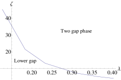
The phase structure of this theory is depicted in Fig. 4. We will elaborate the phase structure in following subsubsections.
3.2.1 Lower gap phase
In the lower gap phase of the critical boson theory, we use the same procedure as the one in section 3.1.1 to obtain the eigenvalue density . We use the cut region and the cut function described in appendix A.1. is same as
| (68) |
because . By substituting the above into (29), we immediately obtain as well as , as
| (69) |
From at the cut with , we obtain the eigenvalue density in the lower gap phase as
| (70) |
At the lower gap phase we get in . By substituing the eigenvalue density (70) into (65) and (66), we can obtain the free energy in the lower gap phase in the critical boson theory.
3.2.2 Upper gap phase
Next we will search for an upper gap solution in the critical boson theory. The cut region and the cut function in this case are defined in appendix A.2. Here the procedure to obtain the eigenvalue density function is the same as the one in subsection 3.1.2. We will take at the upper gap region .
Functions and are obtained based on (29),
| (72) |
Here we use the same definition of as (39). From (72), by taking at the cut region with , we can obtain the eigenvalue density function as
| (73) |
In the region , . By substituing the eigenvalue density (73) into (65) and (66), we can obtain the free energy in the upper gap phase. To derive (73), we have used the formula (41).
3.2.3 Two gap phase
We will search for a two gap solution in the critical boson theory. Our two cuts and the cut function are defined in appendix A.3. By the same procedure as the one in section 3.1.3, we can obtain as well as as
| (75) |
Here is already defined in (44). From , we obtain following two conditions,
| (76) |
and
| (77) |
and are already defined in (45) and (46). By using (77), (76) and (65), are determined as functions of as .
From (75) and by taking at the cuts , we obtain the eigenvalue density function as
| (78) |
Here (78) shares the same definition of with (47). is the same functional form as the eigenvalue density in the GWW model (7.6) in [1]. can be regarded as an additional term depending on the detail of the theory. By substituing the eigenvalue density (78) into (65) and (66), we can obtain the free energy in the two gap phase of the critical boson theory. During the calculation of (78), we have used (76) also.
The combination of (76), (77), (65) and (78) provides a complete set of solutions in the two gap phase.
At large limit, as we proved in appendix C.1.2, the eigenvalue density approaches the universal distribution (16) because remains finite positive quantity at the limit. In the limit, , and the eigenvalue density behave as
| (79) |
At appendix C.2.2, we have demonstrated the above behavior (79). As we can see in the appendix, the eigenvalue density is dominated by at the large limit. The form of the eigenvalue density approaches function which has the same form as Eq. (7.11) in [1], which is the large limit of the eigenvalue density of the GWW model. We can also see that the range of the domain of the cut is smaller than the one in the GWW type matrix integration at the same value of .
3.2.4 Phase transition points
Phase transition from the lower gap to the no gap
Let us consider the behavior of lower gap solutions (71) and (70) at which would correspond to the phase transition points from the lower gap to the no gap. If we substitute into (71), it becomes
| (80) |
This is exactly same as the condition for the phase transition from the no gap to the lower gap phase which is obtained by substituting into eq. (6.24) of [1] and by requiring . Based on this, if we substitute into (70), we obtain
| (81) |
In the last step we have used (80), the Taylor expansion and an integration formula (52). The last line of (81) is exactly same as the eigenvalue distribution in the no gap phase, described at Eq. (6.24) in [1]. So, at the phase transition points, the lower gap solutions are smoothly connected to the the no gap phase solutions.
Phase transition from the upper gap to the no gap
Let us consider the behavior of upper gap solutions (73) and (74) at , which would correspond to the phase transition points from the upper gap to the no gap phase. If we substitute into (74), it becomes
| (82) |
This is exactly same as the condition for the phase transition from the no gap to the upper gap phase discussed in [1], which is obtained by substituting into (6.24) of [1] and by requiring .
Based on this, if we substitute into (73), we can see
| (83) |
In the last step we have used (82), the Taylor expansion and the formula (52). The last line of (83) is exactly same as the eigenvalue distribution in the no gap phase, described at eq. (6.24) in [1]. So, at the phase transition points, the upper gap solutions are smoothly connected to the no gap phase solutions.
Phase transition from the lower gap to the two gap
In the lower gap phase at fixed , if the maximum of the eigenvalue density reaches to , the phase transition from the lower gap phase to the two gap phase will occur. The conditions would be represented in terms of (70) as
| (84) |
The combination of (84), (65) and (71) provides the phase transition points from the lower gap to the two gap. By numerical calculations based on (84), (65) and (71), we obtain the phase transition points plotted in Fig. 5.
Let us see the phase transition points from the standpoint of the two gap phase. If we substitute into (76), it becomes the same as (84), which is the condition of the phase transition points. If we set at (77), it becomes the same as (71). Let us check if the eigenvalue density in the two gap phase (78) becomes the one in the lower gap phase (70) in limit. By using (84), we can replace of (78) by
| (85) |
Then by summing up with , (78) at becomes (70). So, at the phase transition points, we can see that the solutions of two gap phase are smoothly connected to the lower gap phase solutions.
Phase transition from the upper gap to the two gap
In the upper gap phase, if the minimum of the eigenvalue density reaches to , the phase transition from the upper gap phase to two gap phase will occur. The condition would be represented as
| (86) |
The combination of (86), (74) and (65) provides the phase transition points from the upper gap to the two gap. By numerical calculations based on (86), (74) and (65), we obtain the phase transition points plotted in Fig. 5.
Let us see the phase transition points from the standpoint of the two gap phase. If we substitute into (76) it becomes (86) which is the phase transition condition. By using (86), we can see that (77) at is reduced to (74). Let us check that the eigenvalue density in the two gap phase (78) at is smoothly connected to the one in the upper gap phase (73). To confirm it, first we apply the formula (58). Then by using (86) we can rewrite as
| (87) |
Then by summing up with , we can see that (78) at becomes (73). So we can see that the solutions of two gap phase are smoothly connected to solutions of the upper gap phase.
Quadruple phase transition point in the critical boson theory
There is a quadruple phase transition point
| (88) |
at which the four phases coexist. Let us check whether (88) is the quadruple phase transition point or not. Note that (80) is the condition for the phase transition from the no gap to the lower gap phase. Eq. (82) is the the condition for the phase transition between the no gap and the upper gap, (84) is the one between the lower gap and the two gap, and (86) is the one between the upper gap and the two gap. So if (88) satisfies these four equations simultaneously, it becomes the quadruple phase transition point. If we substitute into (84) it becomes
| (89) |
and if we substitute into (86), it also becomes the same equation as (89). We can also see that if both (80) and (82) are simultaneously satisfied, (89) is also automatically satisfied. So if there is a point satisfying (89), the point becomes the quadruple phase transition point. By the study in [1], we already know that only the point (88) simultaneously satisfies both condition (80) and (82). Hence (88) satisfies (89). So (88) becomes the quadruple phase transition point in the critical boson theory. Then due to the existence of the quadruple point, the phase structure of the critical boson theory becomes as in Fig. 4. We can also check that it becomes and at (88), and then the eigenvalue density functions in each phase (70), (73), (78) and (6.24) of [1] coincide.
3.3 Duality between the regular fermion theory and the critical boson theory
In this subsection we will verify the level-rank duality between the level critical boson theory and the level regular fermion theory. We will show that the quantities at in the critical boson theory have duality relationships to the quantities at in the regular fermion theory as
| (90) |
| (91) |
Here the is the eigenvalue density in the regular fermion theory and is the one in the critical boson theory. The relationship between and is
| (92) |
If the above duality relationships (90) (92) are valid, the free energy at in the critical boson theory agrees with the free energy at in the regular fermion theory. So if we verify the above relationships (90) (92), it would be the proof of the level-rank duality between the regular fermion theory and the critical boson theory.
In this subsection, we will first demonstrate the relationships (90) (92) between the lower gap phase of the regular fermion theory and the upper gap phase of the critical boson theory. Next we will verify the relationships between the upper gap phase of the regular fermion theory and the lower gap phase of the critical boson theory. As the third step, we will demonstrate the duality relationships between the two gap phase of both theories. We complete the proof of the relationships (90) (92) between both theories by these three steps. As the final part of this subsection, we will completely verify the duality by evaluating the free energy in both theories.
3.3.1 Between the lower gap phase of regular fermion and upper gap phase of critical boson
Let us define sets of quantities as
| (93) |
Note that the eigenvalue density (73) and the two equations (74), (65) provide a complete set of solutions in the upper gap phase of the critical boson model, while the eigenvalue density (37) and the two equations (38), (32) provide a complete set of solutions in the lower gap phase of the regular fermion theory. So we can verify the duality relationships by checking that becomes a solution provided by the three equations in the regular fermion theory if is a solution provided by the three equations in the critical boson side.
First we will confirm the relationship (90) between the eigenvalue densities (73) and (37) under the correspondence (92),(91). We can show the relationship by directly substituting the (92),(91) into (37) as 999Steps of the calculation to verify (95) are basically combinations of as follows (94) Basically, almost all steps of calculations to verify the duality relationships are just repeating the similar steps to the above. So from here we will not give a blow-by-blow description of similar steps to avoid to be lengthy.
| (95) |
We can also see that becomes a solution of (38) if is a solution of (74) by
| (96) |
You can check this by a straightforward calculation similar to (94).
We will also see that becomes a solution of (32) if is a solution of (65). This is already verified in section 3.6.2 of [1] in the general case. We can check it as follows:
| (97) |
Here we have used
| (98) |
confirmed by the Taylor expansion and .
By the above discussion, we can conclude that becomes a solution provided by the three equations (37), (38) and (32) if is a solution provided by the equations (73), (74), and (65). Thus we have verified the duality relationships between the lower gap phase of the regular fermion theory and the upper gap phase of the critical boson theory.
3.3.2 Between upper gap phase of regular fermion and lower gap phase of critical boson
Let us define sets of quantities as
| (99) |
By similar reasoning to that in section 3.3.1, we can verify the duality relationships by checking that becomes a solution provided by the three equations (40) (42) and (32) in the regular fermion theory if is a solution provided by the three equations (70),(71) and (65) in the critical boson side.
We will confirm the relationship (90) between the eigenvalue densities (70) and (40) under the correspondence (92),(91). By a similar calculation to (94), we can show the relationship (90) as
| (100) |
By checking
| (101) |
in a similar way to (96), we can also see that becomes a solution of (42) if is a solution of (71).
By repeating the analogous calculation to (97), we can see that becomes a solution of (32) if is a solution of (65).
So by the above discussion we can conclude that becomes a solution of the three equations (40), (42) and (32) if is a solution of the equations (70), (71), and (65). Thus we have verified the duality relationships between the upper gap phase of the regular fermion theory and the lower gap phase of the critical boson theory.
3.3.3 Between two gap phases of regular fermion and critical boson theory
Let us define sets of quantities as
| (102) |
By similar reasoning to that in section 3.3.1, we can verify the duality relationships by checking that becomes a solution provided by the four equations (47), (45),(46) and (32) in the regular fermion theory if is a solution provided by the four equations (78),(76), (77) and (65) in the critical boson side.
Correspondence (90) between the eigenvalue density functions
First we will confirm the relationship (90) between the eigenvalue densities (78) and (47) under the correspondence (92),(91). We can directly check
| (103) |
in a similar calculation to (94). From (48), we can see 101010We can see it from (104) These provide the complex line integration along the lower gap.
| (105) |
| (106) |
Here denotes the complex line integration along the upper gap running counterclockwise from to . On the other hand denotes the complex line integration along the lower gap running counterclockwise from to . By using the formula proved in appendix B.2.1,
| (107) |
we can see that
| (108) |
where we use . From (103) and (108), we can confirm the relationship (90) between the eigenvalue densities (78) and (47),
| (109) |
Relationship between (76) and (45)
We will check that becomes a solution of (45) if is a solution of (76). We can easily check
| (110) |
From (48), by a similar calculation to (104), we can see
| (111) |
Here denotes the complex line integration along the upper gap running counterclockwise from to , and denotes the one along the lower gap running counterclockwise from to . From the formula proved in appendix B.2.2, we can see
| (112) |
Hence by taking into account , we can conclude
| (113) |
This (113) shows that becomes a solution of (45) if is a solution of (76).
Relationship between (77) and (46)
We will verify that becomes a solution of the (46) if is a solution of (77). By a straightforward calculation, we can see
| (114) |
From (48), by a similar calculation to (104), we can see
| (115) |
By using the formula shown in appendix B.2.3,
| (116) |
we can see
| (117) |
This (117) shows that becomes a solution of the (46) if is a solution of (77).
Correspondence between (32) and (65)
Summary of the proof
So by the above discussion, we can conclude that becomes a solution provided by the four equations (47),(45),(46) and (32) in the regular fermion theory if is a solution provided by the four equations (78),(76), (77) and (65) at the critical boson side. Thus we have verified the duality relationships at the two gap phase between the regular fermion theory and the critical boson theory.
3.3.4 Relationships between the phase transition points
We have seen that the conditions for the phase transitions (50), (53), (84) etc, can be obtained as a certain limit of corresponding equations between which we have already seen the duality relationships. So we have already shown the duality relationship between the phase transition points, in fact. For example, (84) is obtained by limit of the equation (76) and (57) is obtained by limit of (45). We have already shown that (45) maps to (76) under the duality, moreover we can see . Hence the phase transition points between the upper gap to two gap in the regular fermion maps to the one between the lower gap and the two gap phase in the critical boson theory. Now we will write the phase transition points between the phase to phase in the regular fermion theory as , and the transition points in the critical boson theory as . We can see following dual relationships represented by these symbols
| (118) |
3.3.5 Free energy and completing the proof of the duality
Now we have proved that for any value of , there are duality relationships (90)(92) between the critical boson theory and the regular fermion theory.
Under these correspondences (90)(92), we will show the free energy of the level critical boson theory at (see (66)) agrees with the free energy of the level regular fermion theory at (see (33)),
| (119) |
where can be represented by through the relationship (90).
Under (90) , is expanded in terms of as
| (120) |
By using the periodicity of and by using
| (121) |
we can check
| (122) |
So we can see
| (123) |
under the relationships (90)(92). Now we have completed the proof of the level-rank duality between the level critical boson theory and the level regular fermion theory.
4 Higher temperature phases of the Supersymmetric Chern-Simons matter theory
Next we will study the higher temperature phases of the supersymmetric level Chern-Simons matter theory with a single fundamental chiral multiplet. From here we will call the theory “the SUSY CS matter theory” or “the SUSY theory”. The Lagrangian of the theory we study is presented in equations (2.1) and (3.58) of [25] (see also (6.1) and (6.20) of [9]). From (3.21) of [1], the effective potential in this theory is obtained as
| (124) |
where the thermal mass (for both the boson as well as the fermion in the supermultiplet) is denoted by . The constant above is determined by the requirement that it extremizes ; i.e.
| (125) |
The effective potential can be interpreted as the sum of the regular fermion potential (30) and the critical boson potential (64). So the potential can be written as
| (126) |
where
| (127) |
| (128) |
Hence it is convenient to utilize and combine the results in the previous section to obtain the eigenvalue densities and the free energy in the supersymmetric case. The general form of the free energy of the supersymmetric CS matter theory on is given as
| (129) |
As in the other CS matter theories, to obtain the free energy in each phase, we only have to evaluate the eigenvalue density in each phase and substitute them into (129) and (125). So obtaining the eigenvalue densities in each phase is equivalent to obtaining the free energies in each phase.
The phase structure of this theory is depicted in Fig. 6, as obtained in following subsubsections.
4.1 Lower gap phase
In the lower gap phase of the SUSY CS matter theory, we employ the same procedure as the one in section 3.1.1 to obtain the eigenvalue density . We use the cut region and the cut function defined in appendix A.1. Because , becomes the same as , and we can immediately obtain as well as by substituting the above (130) into (29). Since (29) is linear in , the is obtained as the sum of (36) and (69) with . So is obtained as
| (131) |
4.2 Upper gap phase
To look for the upper gap solution in the current supersymmetric CS matter theory, we only have to follow the same procedure employed in sections 3.1.2 and 3.2.2. The upper cut region as well as the cut function are described in appendix A.2. The function as well as are obtained by using (29), and the function here is evaluated as
| (134) |
Here and are defined in (39), is given in (72). From (134), by taking at the cut region with , we obtain the eigenvalue density function as
| (135) |
where and are defined in (40) and (73) respectively. In the region , . By substituting the eigenvalue density (135) into (125) and (129), we can obtain the free energy in the upper gap phase.
From the condition, , we obtain the equation
| (136) |
4.3 Two gap phase
We will search for a two gap phase solution. We only have to follow the same procedure as the one in section 3.1.3 and 3.2.3. We will take the two cuts region and the cut function defined in appendix A.3. By the same procedure as section 3.1.3, we obtain the functions and as
| (137) |
From this (137), by taking at the cuts , we obtain the eigenvalue density function as
| (138) |
At , and at , . and are defined in (47) and is defined in (78). Similar to (47) and (78), (138) can be interpreted as the sum of GWW type eigenvalue density and other additional terms depending on the details of the theory. By substituting the eigenvalue density (138) into (125) and (129), we can obtain the free energy in the two gap phase of the supersymmetric CS matter theory.
From , we obtain following two conditions,
| (139) |
and
| (140) |
Here and are defined in (45), and is in (76). and are defined in (46) and is in (77).
By using (140), (139) and (125), are determined as functions of as . The combination of (140), (139), (125) and (138) provide a complete set of solutions in the two gap phase of the SUSY CS matter theory.
At the large limit, as we prove in appendix C.1.3, the eigenvalue density approaches the universal distribution (16) because remains finite positive quantity at the limit. In the limit, , and the eigenvalue density behave as
| (141) |
In appendix C.2.3, we have demonstrated the above behavior (141). The eigenvalue density function (138) is dominated by , and approaches , which is the same functional form as (7.11) in [1]. The Eq. (7.11) is the large limit of the eigenvalue density of the GWW model. We can also see that the range of the domain of the cut is smaller than the one in the regular fermion theory as well as the one in the critical boson theory at the same values of .
4.4 Phase transition points
Phase transition from the lower gap to the no gap
Let us consider the behavior of lower gap equations (133) and (132) at which would correspond to the phase transition points from the lower gap to the no gap. If we substitute into (133), it becomes
| (142) |
This is exactly same as the condition for the phase transition from the no gap to the lower gap phase which is obtained by substituting into eq. (6.15) of [1] and by requiring . By using the condition (142), if we substitute into (132), we obtain
| (143) |
This is the same as the eigenvalue density function at the no gap phase of the supersymmetric CS matter theory, which is described by (6.15) of [1]. Also this can be written as the sum of (51) and (81). So the lower gap solutions are smoothly connected to the ones in the no gap phase at the phase transition points.
Phase transition from the upper gap to the no gap
Let us consider the behavior of upper gap solutions (136) and (135) at which would correspond to the phase transition points from the upper gap to the no gap phase. If we substitute into (136), it becomes
| (144) |
This is equivalent to the condition for the phase transition from the no gap to the upper gap phase discussed in [1], which is obtained by substituting into (6.15) of [1] and by requiring . By using (144), the eigenvalue density (135) at becomes
| (145) |
This is the same as the eigenvalue density function at the no gap phase of the SUSY CS matter theory, which is described by (6.15) of [1]. So, at the phase transition points, the upper gap solutions are smoothly connected to the no gap phase solutions.
Phase transition from the lower gap to the two gap
In the lower gap phase at fixed , if the maximum of the eigenvalue density reaches to , the phase transition from the lower gap phase to the two gap phase will occur. The conditions are represented in terms of (132) as
| (146) |
The combination of (146), (125) and (133) provide the phase transition points from the lower gap to the two gap. By numerical calculations based on (146), (125) and (133), we obtain the phase transition points plotted in Fig. 7.
Let us examine the phase transition points from the standpoint of the two gap phase. If we substitute into (139), it becomes (146), and if we set into (140), it becomes the same as (133). Let us check whether the eigenvalue density in the two gap phase (138) becomes the one in the lower gap phase (132) in limit. By using (146) and by similar calculations to (56) and (85), we can confirm that (138) at becomes (132). So we can see that the solutions in the two gap phase are smoothly connected to the ones in the lower gap phase at the phase transition points.
Phase transition from the upper gap to the two gap
In the upper gap phase at fixed , if the minimum of the eigenvalue density reaches to , the phase transition from the upper gap to the two gap phase will occur. The condition is represented in terms of (135) as
| (147) |
The combination of (147), (125) and (136) provide the phase transition points from the upper gap to the two gap. By numerical calculations based on (147), (125) and (136), we obtain the phase transition points plotted in Fig. 7.
Let us examine the phase transition points from the standpoint of the two gap phase. If we substitute into (139) and (140), they become (147) and (136) respectively. By using these correspondence and by using the same procedure as the one in section 3.1.3 and 3.2.3, we can also check that (138) at coincides with (135). So, at the phase transition points, the solutions in the two gap phase are smoothly connected to the upper gap solutions.
Quadruple phase transition points in the SUSY CS matter theory
There is a quadruple phase transition point
| (148) |
at which the four phases coexist. Let us check whether (148) is the quadruple point. Note that (146) is the equation for the phase transition from the lower gap to the two gap. Eq. (147) is the equation for the phase transition from the upper gap to two gap, (142) is the one from the no gap to the lower gap, and (144) is the one from the no gap to the upper gap. So if the point (148) simultaneously satisfies the four equations, it is indeed the quadruple point. We can see that at , (146) as well as (147) become
| (149) |
We can also see that at , (142) and (144) become equivalent to (149). By the study at [1], we already know that both (142) and (144) are simultaneously satisfied at the point (148). So also (149) is satisfied at (148). Then we see that (148) is the quadruple phase transition point in the SUSY CS matter theory. Due to the existence of the quadruple phase transition point, the phase structure becomes as in Fig. 6.
4.5 Self-duality of the SUSY CS matter theory
We will study the self-duality of the supersymmetric CS matter theory under the Giveon-Kutasov type level-rank duality [43, 44]. The level SUSY CS matter theory is dual to the same theory with level gauge group. We will show that there are the following relationships between the quantities in the level theory at and the quantities in the level theory at :
| (150) |
| (151) |
| (152) |
Quantities in the theory are denoted with over-lines while the quantities in the theory are described without over-lines. First we will show the duality between the quantities in the lower gap phase of the theory and the ones in the upper gap phase of the theory. Next we will demonstrate the duality in the two gap phase between the and the theories. At the end of this subsection, we will show the agreement of the free energy under the duality.
4.5.1 Between the lower gap phase of the theory and the upper gap phase of the theory
Let us define sets of quantities
| (153) |
Please note that the the eigenvalue density (132) and the two equations (133), (125) provide a complete set of solutions in the lower gap phase, while the eigenvalue density (135) and (136), (125) provide the one in the upper gap phase. So we can verify the duality relationships by checking that becomes a solution provided by the corresponding three equations in the upper gap phase if is a solution provided by the other three equations in the lower gap.
First we will confirm the relationship (151) between the eigenvalue densities (132) and (135) under the correspondence (150),(152). Here by utilizing relationship (100) and (95), we can check
| (154) |
This shows the relationship (151) between the eigenvalue densities (132) and (135).
We can also see that becomes a solution of (136) if is a solution of (133) by showing
| (155) |
To show this we have used the combination of (96) and (101).
We will also see that the becomes a solution of the (125) if is a solution of it. By using (154), we can directly check as
| (156) |
Here we have used
| (157) |
Eq. (156) shows that becomes a solution of (125) if is a solution of it.
By the above discussion, we can conclude that becomes an upper gap solution provided by the three equations (135), (136) and (125) in the theory if is a lower gap solution provided by the equations (132), (133), and (125) in the theory. Thus we have verified the self-duality relationships between the lower gap phase of the level SUSY CS matter theory and the upper gap phase of the level SUSY CS matter theory.
4.5.2 Self-duality in the two gap phase
Let us define sets of quantities
| (158) |
Here is originally defined as the eigenvalue density function of the dual variable
| (159) |
Please note that the the eigenvalue density (138) and the three equations (139), (140) and (125) provide a complete set of solutions in the two gap phase. So we can verify the duality relationships by checking the following: If is a two gap phase solution of the theory provided by the four equations, also becomes a two gap solution of the theory provided by the same equations.
Correspondence (151) between the eigenvalue density functions
About (139).
About (140).
About (125).
Summary
By the above discussion we can conclude that becomes a solution provided by the four equations (138),(139),(140) and (125) in the level SUSY CS matter theory if is a solution of the same equations in the the level SUSY CS matter theory. Thus we have verified the self-duality relationships at the two gap phase between the level SUSY CS matter theory and the same theory with level gauge group.
4.5.3 Relationships between the phase transition points
We have seen that the conditions for the phase transitions (142), (144), (146) and (147) can be obtained as a certain limit of corresponding equations between which we have already verified the duality relationships. So, by the same logic as in section 3.3.4, we have already shown the duality relationships between the phase transition points. By using the analogous symbols to the ones used in (118), we can see the following duality relationships
| (164) |
4.5.4 Free energy and completing the proof of the duality
Now we have proved that there are self-duality relationships (150)(152) in the SUSY CS matter theory. Under these correspondences (150)(152), we will show that the free energy of the level SUSY CS matter theory at agrees with the free energy of the same theory with level gauge group at , namely,
| (165) |
Here we have used (129). As already shown in (3.30) of [1], by a straightforward calculation similar to (156), we can show . We can also check that by almost the same calculation as (120) and (121).
5 Analytic proof of the duality in the two gap phase of the GWW type matrix integral
In [1], the phase structure of the toy large GWW type matrix integral has been already investigated. Although some numerical evidence have been provided, the analytic proof of the level-rank duality in the two gap phase of the GWW model has not been completed. Then we will complete the analytic proof of the duality by using the three formulae (107), (112) and (116).
This proof would be also useful for analysis of general CS matter theories on . As we can see at (49), (79), (141), and appendix C.2, the eigenvalue densities converge to the one in the GWW model at large limit. Moreover, every eigenvalue density of CS matter theories at the two gap phase includes the term which is the same functional form as the eigenvalue density in the GWW model. So the duality relationships shown in this section play one of the fundamental roles in establishing the level-rank duality in CS matter theories on .
Let us focus on the proof of the level-rank duality in the two gap phase of the GWW model. As described in section C.4 of [1], we can regard as functions of the edge of the cuts . To complete the proof of the self-duality of the GWW type model in terms of this, we should show the following:
| (167) |
| (168) |
| (169) |
If we can verify the above three equations, it becomes the proof of the level-rank duality in the two gap phase of the GWW type matrix integral.
5.1 Proof of (167)
5.2 Proof of (168)
5.3 Proof of (169)
6 Summary and discussions
In this paper, we have elaborated the higher temperature phases of the Chern-Simons matter theories with fundamental representation on . Here we have studied the lower gap, the upper gap and the two gap phases of the regular fermion theory, the critical boson theory, and the supersymmetric Chern-Simons matter theory. We have obtained the eigenvalue density function and the free energy in each phase, and we have also obtained the phase transition points and the phase diagrams. Based on these obtained quantities, we have completely analytically verified the level-rank duality (Giveon-Kutasov type duality) between the regular fermion theory and the critical boson theory, and the self-duality of the SUSY CS matter theory. We have also supplied the analytic proof of the duality in the two gap phase of the GWW type matrix integration which is suggested in [1].
We can see that the proof of the duality in the two gap phase of the GWW model as well as the three formulae (107),(112) and (116) proved in appendix B.2 are based on the cut structure of the two gap phase, which would be shared by all CS matter theories on . Please note that in the eigenvalue density functions at the two gap phase has the same functional form as the eigenvalue density of the GWW model, and it is shared by all the eigenvalue densities in the two gap phase of the all CS matter theories dealt with in this paper. The three formulae play the role of establishing the level-rank duality with respect to the . Hence the duality structure of the GWW model and the three formulae would play the most fundamental role in the level-rank duality of general CS matter theories on .
It is also interesting to compare the three CS matter theories in this paper. As we have seen at (49), (79), (141), and appendix C.2, in the supersymmetric theory, the range of the domain of the cut is smaller than the one in the regular fermion theory as well as the one in the critical boson theory at the same value of . We can also see that the phase transitions at the SUSY theory occur at lower temperatures than the ones in the other two CS matter theories. (See Fig. 8,8.) From this, we can guess that there should be stronger attractive forces between the eigenvalues in the SUSY theory than the one in the other two theories. This may be because the SUSY theory has more degree of freedom of matter fields than the other two theories. Then the effective potential in the SUSY theory obtained after integrating out the matter fields, which causes the attractive force between the eigenvalues, are written by the sum of the ones of the regular fermion and the critical boson theory. Hence the attractive force would be enlarged by the summation.
At the very high temperature limit, the eigenvalue densities of these three theories and the one of the GWW model converge to , and they finally become the same universal distribution (16) if we further increase the temperature. We have given the analysis in (49), (79), (141) and appendix C. So at the very high temperature limit, the results coincide with the ones in [9]. We can regard their results as the very high temperature limit of our results.
It is easy and straightforward to study the critical fermion and the regular boson theory on in the same way as this paper.
One of the interesting application of this paper would be to analyze the phase structure of the dual gravity description governed by parity violating Vasiliev’s higher spin equations [3, 4, 5] at finite values of the ’t Hooft coupling [6, 7]. The thermal system studied in this paper is dual to the Euclidean Vasiliev system in global space compactified on a circle of circumference . The field theory analysis performed in this paper implies that this Vasiliev system admits a classical limit in large limit with with held fixed. The saddle points obtained in this paper should map to classical solutions of this bulk description; however the equations of motion governing this classical description are not necessarily Vasiliev’s equations. This is because quantum corrections to Vasiliev’s equations proportional are not suppressed compared to classical effects in the combined high temperature and large limit studied in this paper; such terms could modify Vasiliev’s classical equations. It would be fascinating to determine the effective 3 dimensional bulk equations dual to the large limit of this paper, and to study the classical solutions dual to the saddle points described in this paper.
Acknowledgments.
The author would like to thank S. Bhattacharyya, S. Jain, S. Minwalla, T. Sharma, S. Wadia, S. Yokoyama for their collaboration in the early stage of this work and helpful discussions. He especially thanks Shiraz Minwalla for reading manuscript and giving helpful comments. He is also really grateful for his TIFR friends’ kind help (D. Bardhan, N. Kundu, A. Lytle, M. Mandlik, T. Sharma and N. Sircar) to correct English grammar. T.T would also like to thank T. Morita for the discussion on the basic part of the matrix model and K. Ohta and H. Suzuki for helpful discussions on the partition function of two dimensional gauge theories in the old days. He would also like to acknowledge our debt to the people of India for their generous and steady support to research in the basic sciences.Appendix A Cut function
We will list the cut region and the cut function in this appendix. The cut region in each phase is depicted in Fig.9, 9 and 9.
A.1 Lower gap case
In the lower gap phase, there is a single cut from , to counterclockwise. As depicted in figure 9, the center of the cut is located at the point 1.
Now let us define the cut function carefully. Let with , then we will define the as
| (178) |
The single cut of this function is taken to lie in an arc on the unit circle extending from to . The function is discontinuous on this arc with
| (179) |
where . Away from this cut (i.e. on the gap) on the unit circle
| (180) | |||||
Recall that everywhere on the gap. On the real axis is everywhere real and is positive for , but is negative for . In particular . In more detail along the real axis
| (181) | |||||
A.2 Upper gap case
Let us consider the case with one upper gap without lower gap. In this case there is a single cut extending from to counterclockwise along the unit circle. The cut centers on the point -1 in the complex plane, see Fig. 9. We can also regard this region as the complement of the cut in the lower gap phase. This interpretation would have important role to show the duality later.
In this case, the function has a branch cut running counterclockwise from to . The function obeys followings:
| (182) |
A.3 Two gap case
In the two gap phase, our two cuts extend along unit circle from to , and from to counterclockwise respectively, see the Fig.9. The cut function in this two gap case will be
| (183) |
where this function has branch cuts along the arcs enumerated above. We will summarize some of properties of the analytic function . Along the unit circle outside the cuts, is analytic as
| (184) | ||||
| (185) |
Along the cuts, becomes discontinuous with
| (186) | ||||
| (187) |
where on the outside of the circle and on the inside. Moreover is real and positive along the real axis; explicitly for real .
| (188) |
Note in particular that . At large we have
| (189) |
Appendix B Important formula
B.1 Important formula in the upper gap phase
In this subsection, we will derive several formulae in the upper gap phase with cut function . This has a branch cut running counterclockwise from to , and has the property (182).
B.1.1 Proof of (43)
Here we will prove the formula (43). Since is everywhere holomorphic except the cuts, from the Cauchy’s theorem
| (190) |
Note that from as ,
| (191) |
then
| (192) |
From first to second line we have used the fact that is holomorphic inside the circle . From the second to third, we have used in the cut region. We finally obtain
| (193) |
B.1.2 Proof of (41)
Here we will prove the formula (41).
Since is everywhere holomorphic except the cut, from the Cauchy’s theorem
| (194) |
From , at ,
| (195) |
so
| (196) |
Here denotes the complex line integration counterclockwise along the cuts. Note that on the cut region, 111111We should note from the standpoint of the counterclockwise complex integration, the sign of the delta function is flipped due to the opposite direction of the integration measure direction.
| (197) |
so it becomes,
| (198) |
We finally obtain
| (199) |
B.2 Important formulae for the proof of level-rank duality in the two gap phase
In this subsection, we will derive several formulae in the two gap phase with cut function s.t.
| (200) |
where this function has branch cuts extending along unit circle from to and from to running counterclockwise. This function satisfies (184) (189). The formulae derived here are important for the proof of the duality in the two gap phase.
B.2.1 Proof of (107)
We will show (107),
| (201) |
where we define as
| (202) |
Throughout this subsection is the arc running counterclockwise along the lower gap on the unit circle, i.e, arc s.t. . is the arc running counterclockwise along the upper gap on the unit circle, i.e, arc s.t. .
Since is holomorphic everywhere except the cut region. Applying the Cauchy’s theorem we get
| (203) |
Since as , we have
| (204) |
From this, we can rewrite
| (205) |
From the first line to second line we have used the fact that is holomorphic inside the circle ,
| (206) |
Note that at the cuts,
| (207) |
and in the upper gap as well as in the lower gap region. Then
| (208) |
So by multiplying to the last line of (208), we obtain (201).
B.2.2 Proof of (112)
Let us prove the formula (112),
| (209) |
Because is holomorphic everywhere except the cuts region, from the Cauchy’s theorem, we get
| (210) |
Using as , we also get
| (211) |
Hence, we can rewrite
| (212) |
From first line to second line, we have used the fact that is holomorphic inside the circle ,
| (213) |
In the last step from the third to the forth line of (212), we have used that in the cuts region while in the gaps region. Hence we can see from the last line of (212),
| (214) |
This completes the proof of (112).
B.2.3 Proof of (116)
Since is holomorphic everywhere except the cuts, from the Cauchy’s theorem, we get
| (215) |
Using as , we also get
| (216) |
Hence
| (217) |
From first line to second line we have used the fact that is holomorphic inside the circle . From the second line to third line we have used the fact that on the cuts region while in the gaps region. From the last line of (217), we can see
| (218) |
This completes the proof of the formula (116)
Appendix C Behavior of eigenvalue distribution at large
We expect that as , with fixed , the eigenvalue densities would behave as
| (219) |
First we will verify that at , with fixed finite , the eigenvalue density in each CS matter theory must be this function. After that we will elaborate more on the behavior of the eigenvalue densities in this limit more.
C.1 Proof of the universal distribution of eigenvalue density at
To verify it, it is useful to note that , at with finite . Here is defined in (45). Note that since
| (220) |
for every , it would be
| (221) |
From (221) we can see that Also in the case of , because of the constraint , is automatically satisfied. So we conclude that
| (222) |
In following subsubsections, we will verify the statement by using (222).
C.1.1 Regular fermion case
If the remains finite in the limit with fixed , from the third line of (45), it follows that remains non-zero finite. Then from the first line of (45), becomes infinite. Hence it follows in the limit with fixed if the remains finite.
To complete the proof we have to show that remains finite in this limit. is given by
| (223) |
The function is positive by the property of as a probability function and by the property that if . At positive we can see the following inequality
| (224) |
Solution of (223) is represented by the the intersection point of the line and in the plane, which is denoted as . From the inequality (224), we immediately see that
| (225) |
is finite quantity for every . 121212We can not apply this analysis for the case . But in case of , the eigenvalue density is always , which already obeys the universal density. So we do not have to mind the case. From this inequality, we can see that the remains positive finite even in the limit with fixed . Hence we have shown that the eigenvalue density becomes universal distribution (219) in the limit .
C.1.2 Critical boson case
We can show in a way similar to the regular fermion case. If the positive number remains finite in the limit with fixed , from the second line of (76), remains non-zero finite. Then from the first line of (76), becomes infinite. Therefore it follows in the limit with fixed , if remains finite.
In order to complete the proof, we have to show that the remains positive finite in the corresponding limit. is given by the following equation
| (226) |
Solution of (226) is represented by the intersection point of the line and in the plane, which is denoted as . Note that at ,
| (227) |
Suppose that is the solution of the equation
| (228) |
from the inequality (224), we can immediately see that
| (229) |
So remains finite even in the limit. Then we have shown that the eigenvalue density becomes universal distribution (219) in the limit with fixed .
C.1.3 SUSY CS matter theory case
We can show in a way similar to the previous cases. As in the previous cases, if the positive number remains finite in the limit with fixed , from the second line of (139), remains non-zero finite. Then from the first line of (139), becomes infinite. Hence it follows in the limit with fixed , if the remains finite.
In order to complete the proof, we have to show that the remains finite at the corresponding limit. The is given by the equation
| (230) |
For any , , we see the following inequality,
| (231) |
Note that the last term is independent of . Suppose that is the solution of the equation
| (232) |
due to the inequality (231), we see
| (233) |
Hence we conclude the positive remains finite even in the limit , then we have shown that the eigenvalue density becomes the universal distribution (219) in the limit with fixed .
C.2 Behavior of eigenvalue density in large limit, with
We will elaborate how the eigenvalue density deviates from the universal distribution (219) if we gradually decrease the temperature from .
C.2.1 Regular fermion theory
To consider the behavior in the regular fermion theory, we should evaluate behavior of the combination of (45), (46) and (32) at large where with . (As in section C.2 in [1].) In this limit, these three equations can be expanded as in to give
| (234) |
and
| (235) |
and
| (236) |
respectively. From these we can obtain and as
| (237) | ||||
| (238) |
Since
| (239) |
is estimated as from (237).
Let us consider the asymptotic behavior of the eigenvalue density (47) in limit. Here of (47) is the same functional form as the one in the GWW type model (7.6) of [1], while of (47) is regarded as an additional term appearing in the regular fermion theory. We can see that falls off as . On the other hand remains finite. So in the limit, becomes
| (240) |
where where . This behavior is very similar to the one in the GWW type model, (7.11) of [1].
Although the functional form of in the large limit is almost same as the one in the GWW type model, the range of in the regular fermion theory would be different from in the GWW type model. To evaluate the , we should calculate the factor in (237), and compare with in the GWW case. By numerical calculations, we can confirm that
| (241) |
for every value of . We plot the function in Fig. 11. Hence we see that at of the regular fermion theory (237) is smaller than at the same of GWW model. This means that the shape of the eigenvalue density function of the regular fermion theory has a sharper cliff than the one in GWW model. (Schematic graph of the eigenvalue density is depicted at Fig. 10.)
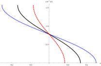
C.2.2 Critical boson theory
Also in the critical boson theory, we consider how the eigenvalue density deviates from universal configuration (219) as we decrease the temperature.
To consider the behavior, we should investigate the combination of the conditions (76), (77), and (65) in the large where with . In this limit, the asymptotic behavior of these three equations are
| (242) |
and
| (243) |
and
| (244) |
respectively. From these, and are evaluated as
| (245) | ||||
| (246) |
Since
| (247) |
is evaluated as from (245).
Let us consider the asymptotic behavior of the eigenvalue density (78) in limit. Here of (78) is the same functional form as the one in the GWW type model (7.6) of [1], while of (78) is regarded as an additional term appearing in the critical boson theory. We can see that falls off as . On the other hand remains finite. So in this limit, becomes
| (248) |
This behavior is also very similar to the one in the regular fermion case as well as the one in the GWW type (7.11) of [1].
The range of in the critical boson theory would also be different from in the GWW type model. To evaluate the , we should calculate the factor in (245), and compare with in the GWW case. By numerical calculations, we confirm that
| (249) |
for every value of . (See the plots of in Fig. 11). This means that the shape of the eigenvalue density function of the critical boson theory has a sharper cliff than the one in GWW model. (Schematic graph of the eigenvalue density is depicted at Fig. 10.) We can see that in (245) as well as are dual to in (237) and under the level-rank duality. We can also see the duality between and from the graph Fig. 11.
C.2.3 Supersymmetric CS matter theory
Similar to the other cases, we consider the behavior of the combination of (139), (140) and (125) at large . In this limit these behave as
| (250) |
and
| (251) |
and
| (252) |
From these, and are evaluated as
| (253) | |||||
| (254) |
Since
| (255) |
we can see
Let us consider the asymptotic behavior of the eigenvalue density (138) in the limit. Here of (138) is the same functional form as the one in the GWW type model (7.6) of [1], while of (138) is regarded as an additional term appearing in the SUSY CS matter theory. We can see that falls off as . On the other hand remains finite. So in the limit, becomes
| (256) |
This behavior is very similar to other CS matter theories.
The range of in the SUSY CS matter theory would be the smallest among the CS matter theories which we have already studied in this paper. We can estimate by calculating the factor in (253). (The plots of is in Fig. 11). From this, we can see . This means that in the SUSY CS matter theory is the smallest and shape of the eigenvalue density function of the SUSY CS matter theory has the sharpest cliff among the CS matter theories. (Schematic graph of the eigenvalue density is depicted at Fig. 10.) We can see that at (253) as well as are self-dual under the level-rank duality. We can also see the self-duality of from the graph Fig. 11.
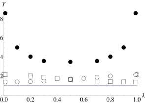
References
- [1] S. Jain, S. Minwalla, T. Sharma, T. Takimi, S. R. Wadia, et. al., Phases of large vector Chern-Simons theories on , arXiv:1301.6169.
- [2] I. Klebanov and A. Polyakov, AdS dual of the critical O(N) vector model, Phys.Lett. B550 (2002) 213–219, [hep-th/0210114].
- [3] M. A. Vasiliev, Consistent equation for interacting gauge fields of all spins in (3+1)-dimensions, Phys.Lett. B243 (1990) 378–382.
- [4] M. Vasiliev, Nonlinear equations for symmetric massless higher spin fields in (A)dS(d), Phys.Lett. B567 (2003) 139–151, [hep-th/0304049].
- [5] S. Giombi and X. Yin, The Higher Spin/Vector Model Duality, arXiv:1208.4036.
- [6] S. Giombi, S. Minwalla, S. Prakash, S. P. Trivedi, S. R. Wadia, et. al., Chern-Simons Theory with Vector Fermion Matter, Eur.Phys.J. C72 (2012) 2112, [arXiv:1110.4386].
- [7] C.-M. Chang, S. Minwalla, T. Sharma, and X. Yin, ABJ Triality: from Higher Spin Fields to Strings, arXiv:1207.4485.
- [8] E. Witten, Anti-de Sitter space, thermal phase transition, and confinement in gauge theories, Adv.Theor.Math.Phys. 2 (1998) 505–532, [hep-th/9803131].
- [9] O. Aharony, S. Giombi, G. Gur-Ari, J. Maldacena, and R. Yacoby, The Thermal Free Energy in Large N Chern-Simons-Matter Theories, arXiv:1211.4843.
- [10] M. R. Douglas and V. A. Kazakov, Large N phase transition in continuum QCD in two-dimensions, Phys.Lett. B319 (1993) 219–230, [hep-th/9305047].
- [11] X. Arsiwalla, R. Boels, M. Marino, and A. Sinkovics, Phase transitions in q-deformed 2-D Yang-Mills theory and topological strings, Phys.Rev. D73 (2006) 026005, [hep-th/0509002].
- [12] N. Caporaso, M. Cirafici, L. Griguolo, S. Pasquetti, D. Seminara, et. al., Topological strings and large N phase transitions. I. Nonchiral expansion of q-deformed Yang-Mills theory, JHEP 0601 (2006) 035, [hep-th/0509041].
- [13] D. Jafferis and J. Marsano, A DK phase transition in q-deformed Yang-Mills on S**2 and topological strings, hep-th/0509004.
- [14] A. Kapustin, B. Willett, and I. Yaakov, Nonperturbative Tests of Three-Dimensional Dualities, JHEP 1010 (2010) 013, [arXiv:1003.5694].
- [15] A. Kapustin, B. Willett, and I. Yaakov, Tests of Seiberg-like Duality in Three Dimensions, arXiv:1012.4021.
- [16] O. Aharony, G. Gur-Ari, and R. Yacoby, d=3 Bosonic Vector Models Coupled to Chern-Simons Gauge Theories, JHEP 1203 (2012) 037, [arXiv:1110.4382].
- [17] O. Aharony, G. Gur-Ari, and R. Yacoby, Correlation Functions of Large N Chern-Simons-Matter Theories and Bosonization in Three Dimensions, arXiv:1207.4593.
- [18] E. Ivanov, Chern-Simons matter systems with manifest N=2 supersymmetry, Phys.Lett. B268 (1991) 203–208.
- [19] D. Gaiotto and X. Yin, Notes on superconformal Chern-Simons-Matter theories, JHEP 0708 (2007) 056, [arXiv:0704.3740].
- [20] R. D. Pisarski and S. Rao, Topologically Massive Chromodynamics in the Perturbative Regime, Phys.Rev. D32 (1985) 2081.
- [21] W. Chen, G. W. Semenoff, and Y.-S. Wu, Two loop analysis of nonAbelian Chern-Simons theory, Phys.Rev. D46 (1992) 5521–5539, [hep-th/9209005].
- [22] J. Maldacena and A. Zhiboedov, Constraining Conformal Field Theories with A Higher Spin Symmetry, arXiv:1112.1016.
- [23] J. Maldacena and A. Zhiboedov, Constraining conformal field theories with a slightly broken higher spin symmetry, arXiv:1204.3882.
- [24] S. Banerjee, S. Hellerman, J. Maltz, and S. H. Shenker, Light States in Chern-Simons Theory Coupled to Fundamental Matter, arXiv:1207.4195.
- [25] S. Jain, S. P. Trivedi, S. R. Wadia, and S. Yokoyama, Supersymmetric Chern-Simons Theories with Vector Matter, JHEP 1210 (2012) 194, [arXiv:1207.4750].
- [26] S. Yokoyama, Chern-Simons-Fermion Vector Model with Chemical Potential, arXiv:1210.4109.
- [27] S. Banerjee, A. Castro, S. Hellerman, E. Hijano, A. Lepage-Jutier, et. al., Smoothed Transitions in Higher Spin AdS Gravity, arXiv:1209.5396.
- [28] G. Gur-Ari and R. Yacoby, Correlators of Large N Fermionic Chern-Simons Vector Models, arXiv:1211.1866.
- [29] S. H. Shenker and X. Yin, Vector Models in the Singlet Sector at Finite Temperature, arXiv:1109.3519.
- [30] M. Blau and G. Thompson, Derivation of the Verlinde formula from Chern-Simons theory and the G/G model, Nucl.Phys. B408 (1993) 345–390, [hep-th/9305010].
- [31] D. Gross and E. Witten, Possible Third Order Phase Transition in the Large N Lattice Gauge Theory, Phys.Rev. D21 (1980) 446–453.
- [32] S. R. Wadia, A Study of U(N) Lattice Gauge Theory in 2-dimensions, arXiv:1212.2906.
- [33] S. R. Wadia, N = infinity phase transition in a class of exactly soluble model lattice gauge theories, Phys.Lett. B93 (1980) 403.
- [34] B. Sundborg, The Hagedorn transition, deconfinement and N=4 SYM theory, Nucl.Phys. B573 (2000) 349–363, [hep-th/9908001].
- [35] O. Aharony, J. Marsano, S. Minwalla, K. Papadodimas, and M. Van Raamsdonk, The Hagedorn - deconfinement phase transition in weakly coupled large N gauge theories, Adv.Theor.Math.Phys. 8 (2004) 603–696, [hep-th/0310285].
- [36] O. Aharony, J. Marsano, S. Minwalla, K. Papadodimas, and M. Van Raamsdonk, A First order deconfinement transition in large N Yang-Mills theory on a small S**3, Phys.Rev. D71 (2005) 125018, [hep-th/0502149].
- [37] O. Aharony, J. Marsano, and M. Van Raamsdonk, Two loop partition function for large N pure Yang-Mills theory on a small S**3, Phys.Rev. D74 (2006) 105012, [hep-th/0608156].
- [38] K. Papadodimas, H.-H. Shieh, and M. Van Raamsdonk, A Second order deconfinement transition for large N 2+1 dimensional Yang-Mills theory on a small two-sphere, JHEP 0704 (2007) 069, [hep-th/0612066].
- [39] M. Mussel and R. Yacoby, The 2-loop partition function of large N gauge theories with adjoint matter on S**3, JHEP 0912 (2009) 005, [arXiv:0909.0407].
- [40] L. Alvarez-Gaume, C. Gomez, H. Liu, and S. Wadia, Finite temperature effective action, AdS(5) black holes, and 1/N expansion, Phys.Rev. D71 (2005) 124023, [hep-th/0502227].
- [41] L. Alvarez-Gaume, P. Basu, M. Marino, and S. R. Wadia, Blackhole/String Transition for the Small Schwarzschild Blackhole of AdS(5)x S**5 and Critical Unitary Matrix Models, Eur.Phys.J. C48 (2006) 647–665, [hep-th/0605041].
- [42] M. R. Douglas, Chern-Simons-Witten theory as a topological Fermi liquid, hep-th/9403119.
- [43] A. Giveon and D. Kutasov, Seiberg Duality in Chern-Simons Theory, Nucl.Phys. B812 (2009) 1–11, [arXiv:0808.0360].
- [44] F. Benini, C. Closset, and S. Cremonesi, Comments on 3d Seiberg-like dualities, JHEP 1110 (2011) 075, [arXiv:1108.5373].