The Rise and Fall of R&D Networks

Abstract

Drawing on a large database of publicly announced R&D alliances, we empirically investigate the evolution of R&D networks and the process of alliance formation in several manufacturing sectors over a 24-year period (1986-2009). Our goal is to empirically evaluate the temporal and sectoral robustness of a large set of network indicators, thus providing a more complete description of R&D networks with respect to the existing literature. We find that most network properties are not only invariant across sectors, but also independent of the scale of aggregation at which they are observed, and we highlight the presence of core-periphery architectures in explaining some properties emphasized in previous empirical studies (e.g. asymmetric degree distributions and small worlds). In addition, we show that many properties of R&D networks are characterized by a rise-and-fall dynamics with a peak in the mid-nineties. We find that such dynamics is driven by mechanisms of accumulative advantage, structural homophily and multiconnectivity. In particular, the change from the “rise” to the “fall” phase is associated to a structural break in the importance of multiconnectivity.

1 Introduction

This work investigates the structural properties of empirical R&D networks and the rules of alliance formation by firms. In several industries, and especially in those with rapid technological growth, innovation relies on general and abstract knowledge often built on scientific research (Powell et al.,, 1996; Dosi,, 1993). This has allowed for a division of innovative labor and fostered collaboration across firms (Arora and Gambardella, 1994b, ; Arora and Gambardella, 1994a, ; Dosi,, 1995). Accordingly, the last three decades have witnessed a significant growth in the number of formal and informal R&D collaborations (e.g. Hagedoorn,, 2002; Powell et al.,, 2005), and several studies have documented the importance of networks for knowledge spillovers and firms’ innovative performance (see e.g. Powell et al.,, 1996; Ahuja,, 2000; Giuliani,, 2007)

The growing importance of R&D networks has resulted in a signficant amount of empirical research about the structural properties of those networks and on the determinants of their evolution. On the one hand, these empirical works have shown that R&D networks are typically sparse and characterized by heavily asymmetric distributions of the number of alliances (e.g. Powell et al.,, 2005; Rosenkopf and Schilling,, 2007; Hanaki et al.,, 2010). Furthermore, R&D networks exhibit the so-called small world property (as shown by Fleming and Marx,, 2006; Fleming et al.,, 2007), i.e. they are characterized by short average path length and high clustering (Watts and Strogatz,, 1998). On the other hand, another group of empirical studies (see e.g. Gulati et al.,, 2012; Powell et al.,, 2005; Rosenkopf and Padula,, 2008; Gulati, 1995b, ) has proposed and tested models for the process of alliance formation driving the evolution of R&D networks. This latter research stream is firmly rooted on the idea that the process of network evolution is strongly path-dependent. In that, the existing structures of the network, and the position of the firms therein, capture different technological as well as social and organizational characteristics, and shape firms’ decisions about future creation and deletion of alliances.

The above empirical studies have greatly contributed to the understanding of empirically observed R&D networks. However, they have often focused only on a small number of industries and/or they have rarely considered how the properties of the network may evolve over time. Finally, they have focused on a small set of network measures (e.g. size, degree heterogeneity, small world properties), which limits the understanding of the path-dependent process of alliance formation.

On these premises, our work improves on the foregoing literature along several dimensions. First, we analyze a global inter-firm R&D network (the pooled R&D network), as well as its decomposition in a series of subnetworks for several representative manufacturing sectors (the sectoral R&D networks). Through such an analysis, we are able to check whether the network properties that have been analyzed by the current literature for sectors like computers (e.g. Hanaki et al.,, 2010) or pharmaceuticals (e.g. Powell et al.,, 2005) are robust across different sectors of activity. In addition, by comparing the properties at the pooled and at the sectoral levels, we are able to check for the presence of universal properties of R&D networks that hold irrespectively of the scale of aggregation at which they are observed.

Second, we investigate a broad set of network properties. The object of our analysis are not only the basic measures that have so far been considered in the empirical literature (size, degree heterogeneity, small world properties), but also indicators related to more complex features of the network, such as assortativity (i.e. the presence of positive correlation in the number of alliances among firms; see also Newman,, 2003) and the presence of “nested” core-periphery architectures (see Bascompte et al.,, 2003). In this way, we refine the existing knowledge on R&D networks by detecting new stylized facts about the structural features of those networks and shed further lights on the drivers of the process of alliance formation.

Third, building on the above-mentioned structural analysis, we perform a longitudinal analysis of the determinants of R&D alliance formation. In this analysis, our dependent variable is a firm dyad, and the observation unit is every potential pair of firms in the R&D network. We then investgate which combination of attachment rules provides a good description of the empirical evolution of alliances in the sample considered. We focus on the mechanisms of alliance formation which have received more attention in the literature so far, namely: (i) accumulative advantage, (ii) structural homophily (or diversity) and (iii) multiconnectivity (see Rosenkopf and Padula,, 2008; Powell et al.,, 2005). Moreover, we conduct regression analyses for different time periods. In this way we are able to check if different attachment rules may account for different evolutions of the network over the observed sample. Finally, we also consider separately alliances formed among incumbent firms in the network, and alliances where at least one firm is entering the network, in order to check whether drivers of alliance formation are different across incumbents and entrants.

Our results show, first, that the evolution of R&D networks has been universal across different scales of aggregation. Indeed, many structural properties of the network (e.g. asymmetric degree distributions, assortativity, presence of small worlds) robustly hold both when alliances are considered irrespectively of the sectors of the firms and when sectoral networks are analyzed. Second, we show that the dynamics of R&D networks has been characterized by two distinctive phases: in the first of them (the “rise” phase, from 1986 to 1997), alliances gave rise to dense network structures, organized into very few large components displaying core-periphery nested architectures. In the second phase (the “fall” phase, from 1998 to 2009), networks become more sparse and fragmented into many small components with few firms. Third, our regression results bring support to the idea that the process of alliance formation has largely been driven by accumulative advantage and by the search for similar partners (“homophily”). Moreover, we find that in the rise phase firms also tried to form alliances to increase the number of paths through which other firms could be directly or indirectly reached (“multiconnectivity”), whereas in the fall phase such an alliance driver lost significance. In turn, such a structural break in the importance of multiconnectivity underlies the emergence of densely connected networks and their subsequent fragmentation.

Our results have several implications. First, the universality of the structural properties of the network reinforces the idea that R&D alliances can be analyzed independently of the characteristics of the sectors to which firms belong, and by focusing on simple rules of alliance formation capturing different organizational and technological drivers, given the existing network structure. Second, our findings on the rise and fall of the networks confirm previous results about the presence of a life-cycle in the evolution of networks (see in particular Gulati et al.,, 2012). At the same time, they show that such a dynamics is not specific to a single industry but is rather a general property of many sectoral networks and it also holds independently of the scale of aggregation. In addition, the finding that network components are organized into core-periphery architectures in the rise phase is able to jointly explain two features that have so far received a great deal of attention in the empirical literature, namely the presence of small worlds and fat-tailed degree distributions. Finally, and in line with Powell et al., (2005), our results show that multiconnectivity matters besides more traditional drivers of R&D alliances, and in particular to explain structural breaks in the R&D network evolution.

The paper is organized as follows. Section 2 describes the data and the methodology used to build the networks of R&D alliances. Section 3 presents a set of basic network properties, such as size, density, the emergence of a giant component, and discusses their evolution over time. Section 4 studies the heterogeneity and the homophily in the network, by analyzing degree distributions and degree correlations (assortativity). Section 5 studies the emergence of small-world and nested core-periphery structures in the R&D networks. Section 6 investigates the determinants of alliance formation through a set of regression models, discussing the results in light of the existing theoretical and empirical literature on R&D networks. Finally, Section 7 concludes. The Appendix contains a description of all network measures used in the paper.

2 R&D alliance data and the construction of R&D networks

An R&D network is a representation of the research and development alliances occurring between firms in one or more industrial sectors within a given period. Every network consists of a set of nodes and links connecting pairs of nodes. In our representation, each node of the network is a firm and every link represents an R&D alliance between two firms. By R&D alliance, we refer to an event of partnership between two firms, that can span from formal joint ventures to more informal research agreements, specifically aimed at research and development purposes. To detect such events, we use the SDC Platinum database, provided by Thomson Reuters, that reports all publicly announced alliances, from 1984 to 2009, between several kinds of economic actors (including manufacturing firms, investors, banks and universities). We then select all the alliances concerning manufacturing firms and displaying the “R&D” tag; after applying this filter, we obtain a total of 8,835 listed alliances.

Information in the SDC dataset is gathered only from announcements in public sources, such as press releases or journal articles. Nevertheless, despite the bias that could be introduced by such a collection procedure, Schilling, (2009) shows that the SDC Thomson dataset provides a consistent picture with respect to alternative databases (e.g. CORE and MERIT-CATI, see also Hagedoorn et al.,, 2000) in terms of alliance activity over time, industry composition and geographical location of companies. The country coverage of the SDC dataset is also consistent with the alternative datasets: 55% of the listed firms are registered in the U.S.A., 8.5% in Japan, 4.4% in Canada, 4.3% in the U.K. and so on. See Table 1 for more details.

	Number of firms	Fraction
Pooled	9499	1.000
United States	5245	0.552
Japan	804	0.085
Canada	421	0.044
United Kingdom	411	0.043
Germany	358	0.038
China	331	0.035
France	236	0.025
Australia	202	0.021
India	119	0.013
Italy	109	0.011
Other	1263	0.133

Table 1: Network composition with respect to the geographical provenience of the firms listed in our dataset. The top-ten represented countries account for 87% of all listed firms.

We check all firm names and control for all legal extensions (e.g. “ltd”, “inc”, etc.) and other recurrent keywords (e.g. “bio”, “tech”, “pharma”, “lab”, etc.) that could affect the matching between entries referring to the same firm. We keep as separated entities the subsidiaries of the same firm located in different countries. The raw dataset contains a total of 16,313 firms, which are reduced to 9,499 after running such an extensive standardization procedure.

In our network representation, we draw a link connecting two nodes every time an alliance between the two corresponding firms is announced in the dataset. An alliance is associated with an undirected link, as we do not have any information about the initiator of the alliance. When an alliance involves more than two firms (consortium), all the involved firms are connected in pairs, resulting into a fully connected clique. Following this procedure, the 8,835 alliance events listed in the dataset result in a total of 11,827 links. Similarly to Rosenkopf and Schilling, (2007), the R&D network that we consider in our study is unipartite, as we only have one set of actors (“the firms”), whose elements may be connected – or not – by publicly announced alliances.

Multiple links between the same nodes are in principle allowed (two firms can have more than one alliance on different projects). Nevertheless, as we aim at studying the connections between firms, and not the number of alliances a firm is involved in, we discard this information and use unweighted links in our network representation. For this reason, we define the degree of a node as the number of other nodes to which it is linked, i.e. the number of partners that a firm has – not the number of alliances. Furthermore, a firm appears in the R&D network only if it is involved in at least one alliance. Our study is focused exclusively on the embeddedness of firms into an alliance network; for this reason, isolated nodes are not part of our network representation.

Both the links and the nodes of the R&D network are characterized by an entry/exit dynamics. Alliances between firms have a finite duration (see Deeds and Hill,, 1999; Phelps,, 2003). This causes some firms to disappear from the network, after they no longer participate in any alliance. Likewise, many new firms that are not listed in any previous alliance may enter the network at the beginning of a new year. Our longitudinal study obviously requires precise temporal information about the formation and the deletion of alliances. The SDC Platinum dataset contains the beginning date of every alliance, but there is no information about any of the ending dates (firms do not usually organize press releases to announce the end of an alliance). We are thus forced to make some assumptions about the alliance durations. We draw the duration of every alliance from a normal distribution with mean value from 1 to 5 years and standard deviation from 1 to 5 years, and we find that all our results remain qualitatively unchanged within these ranges. Given the strong robustness of the R&D network to the variation of alliance lengths, we take a conservative approach and assume a fixed 3-year length for every partnership, consistently with previous empirical work (e.g. Rosenkopf and Schilling,, 2007; Phelps,, 2003; Deeds and Hill,, 1999). More precisely, we link two nodes when an alliance between the corresponding firms occurs and we delete this link 3 years after its formation. This is also the reason why, even though our dataset starts reporting R&D alliances from the year 1984, we start building the corresponding R&D network from the year 1986. In this way, we are able to build 26 snapshots of the R&D network – one for every year – from 1986 to 2009. From now on we call the network containing all companies, irrespectively of their industrial sector, the pooled R&D network.

Every firm in the dataset is associated to a SIC code (Standard Industrial Classification). This allows us to build a series of sectoral R&D networks, one for each sector that we identify in the dataset. A sectoral R&D network contains only alliances in which at least one of the partners has a three-digit SIC code matching the selected sector (see also Rosenkopf and Schilling,, 2007, for a similar approach). The rules for link deletion are the same as in the pooled R&D network. More precisely, we focus on the 10 largest manufacturing sectors (in terms of numbers of firms in the network). Table 2 provides the list of the sectors considered, together with the number of reported firms and alliances, both in absolute and in relative terms.

	Number of firms	(fraction)	Number of alliances	(fraction)
Pooled	9499	1.000	8835	1.000
Pharmaceuticals	2224	0.234	2576	0.292
Computer Software	1826	0.192	1533	0.174
Electronic Components	596	0.063	787	0.089
Computer Hardware	498	0.052	741	0.084
Medical Supplies	439	0.046	285	0.032
Communications Equipment	436	0.046	399	0.045
Laboratory Apparatus	301	0.032	207	0.023
Motor Vehicles	243	0.026	240	0.027
Inorganic Chemicals	147	0.015	129	0.015
Aircrafts and parts	146	0.015	132	0.015
Other	2643	0.278	1805	0.204

Table 2: Network composition with respect to the industrial sectors. The top-ten represented sectors account for 72% of all listed firms and 80% of all listed alliances. Note: when an alliance event involves firms from different sectors, the weight of the alliance is equally distributed between the partners.

We study both the pooled R&D network and the sectoral R&D networks by computing a set of network indicators along the whole observation period. We group our descriptive analysis of the network into three sections. We begin by discussing basic facts about the evolution of the network, such as its size, density and connectedness. Next, we discuss the degree of heterogeneity and homophily in the network, by studying the evolution of the degree distributions and of assortativity patterns. Finally, we discuss how network components are organized, by studying the presence of small worlds and of core-periphery structures.

3 Basic facts about the evolution of R&D networks

We begin our analysis by discussing some basic properties concerning the evolution of the pooled R&D network. Following Powell et al., (2005); Rosenkopf and Schilling, (2007); Rosenkopf and Padula, (2008) we employ network visualization techniques to provide a first assessment of how network structures evolved over the years analyzed. More precisely, Figures 1 and 2 show several snapshots of, respectively, the pooled and five sectoral networks. The plots are produced using the igraph library for R, and the networks are displayed using the Fruchterman-Reingold algorithm (cf. Fruchterman and Reingold,, 1991). This is a force-based algorithm for network visualization which positions the nodes of a graph in a two-dimensional space so that all the edges are of similar length and there are as few crossing edges as possible. The result is that the most interconnected nodes are displayed close to each other in the resulting two-dimensional plot. We use node colors to identify the sectors to which firms belong. More precisely, in Figure 1 each different color indicates a different sector. In Figure 2, instead, different colors indicate whether the firm belongs to the same sector on which the network is centered or not. This is in order to provide a visual indication on the share of intra-sectoral and inter-sectoral alliances in each industry.

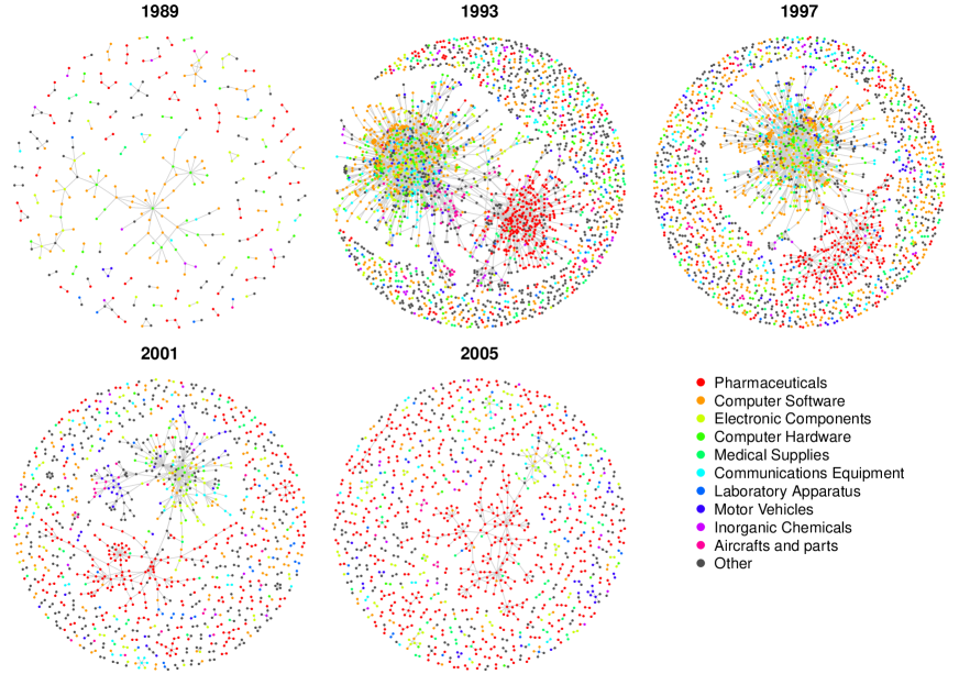
Figure 1: Evolution of the pooled R&D network. Pooled R&D network snapshots in 1989, 1993, 1997, 2001 and 2005. In order to ease the visualization, we only plot the nodes belonging to the ten largest sectors and their alliance partners.

Figure 1 denotes the presence of different phases in the evolution of the R&D network. The plots suggest a significant growth of the network until 1997, and a reversal of this trend aftermath. Interestingly, such a rise-and-fall pattern is also present in sectoral networks. Indeed, Figure 2 shows that – although with different intensities – all plotted sectors display a concentration of alliance activities in 1993 and 1997, followed by a decline in the number of alliances in the 2000s decade. Incidentally, notice that the same rise-and-fall dynamics is displayed by sectors which are very different in terms of technological characteristics (e.g. Pharmaceutical and Aircrafts and Parts, see Rosenkopf and Schilling,, 2007).

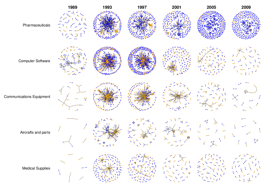
Figure 2: Evolution of five selected sectoral R&D networks. Snapshots in 1989, 1993, 1997, 2001, 2005 and 2009 for five selected sectoral R&D networks: Pharmaceuticals, Computer Software, Communication Equipments, Aircrafts and parts, Medical Supplies. Blue nodes represent the firms strictly belonging to the examined sector, while orange nodes represent their alliance partners belonging to different sectors.

Figure 3 provides important additional elements about the network dynamics in our sample. The figure shows the evolution of the network density (number of existing links divided by the number of all possible links in the network) and the network size of the pooled network, and shows quite starkly that the growth in the size of the network has been associated to a significant fall in its density. This means that the expansion of the R&D network was heavily driven by new alliances created by entrant firms. Moreover, after the “golden age”, the fall of the network has been associated with a decrease in the number of nodes. Because of the importance of entry in the observed R&D network dynamics, in Section 6 we perform separate regression analyses to investigate the determinants of the formation of alliances by entrants.

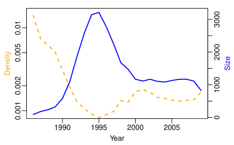
Figure 3: Size and density evolution of the pooled R&D network. Time-evolution of size (solid line, right y-axis) and density (dashed line, left y-axis) of the pooled R&D network. Note that the density is visualized on a logarithmic scale.

Another interesting feature of network dynamics in our sample is the emergence of densely connected giant components, both at the pooled and sectoral level. This is evident not only from the plots in Figures 1 and 2, but also from the time-evolution of the number of firms in such components, and reported in Table 4. The emergence of a giant component in the network is of particular interest, as both previous empirical and theoretical works (e.g. Powell et al.,, 2005; Goyal and Joshi,, 2003; König et al.,, 2012) have stressed that high network connectedness favors technological spillovers and overall knowledge growth by increasing the number of knowledge sources to which single firms have direct or indirect access via alliances. Figure 1 also shows significant heterogeneity in terms of the type of sectors present in the giant component although two categories of sectors seems to be prevalent in the component: pharmaceuticals and ICT-related sectors (computer software and hardware, electronic components, communications equipment). The foregoing giant component has then significantly shrunk in the 2000s, leaving space to a growing periphery of disconnected dyads (pairs of allied firms). Such a process of increasing connectedness and subsequent fragmentation of the network is present also at the sectoral level (see Figure 2), although the intensity of the network fragmentation in the 2000s looks much lower in pharmaceuticals than in the other plotted sectors.

	1986-1989	1990-1993	1994-1997	1998-2001	2002-2005	2006-2009
Pooled	207	1529	2846	1358	1122	1069
Pharmaceuticals	63	440	617	461	508	666
Computer Software	74	485	1145	406	198	94
Electronic Components	66	312	528	246	188	144
Computer Hardware	65	372	650	208	90	40
Medical Supplies	10	142	236	120	86	111
Communications Equipment	26	210	408	172	104	51
Laboratory Apparatus	22	148	225	118	84	65
Motor Vehicles	15	104	178	104	89	69
Inorganic Chemicals	18	100	132	54	41	32
Aircrafts and parts	12	82	127	65	42	24

Table 3: Network size for the pooled and the sectoral R&D networks. The values are averages within each sub-period.

	1986-1989	1990-1993	1994-1997	1998-2001	2002-2005	2006-2009
Pooled	0.112	0.507	0.536	0.367	0.179	0.216
Pharmaceuticals	0.107	0.583	0.663	0.495	0.240	0.334
Computer Software	0.287	0.664	0.613	0.354	0.244	0.096
Electronic Components	0.152	0.665	0.726	0.583	0.387	0.106
Computer Hardware	0.257	0.681	0.757	0.652	0.526	0.152
Medical Supplies	0.254	0.189	0.294	0.117	0.091	0.061
Communications Equipment	0.222	0.665	0.697	0.577	0.400	0.181
Laboratory Apparatus	0.242	0.439	0.372	0.311	0.181	0.088
Motor Vehicles	0.289	0.537	0.529	0.472	0.311	0.098
Inorganic Chemicals	0.253	0.373	0.408	0.147	0.231	0.266
Aircrafts and parts	0.483	0.628	0.463	0.355	0.237	0.152

Table 4: Fraction of the giant component for the pooled and the sectoral R&D networks. The values are averages within each sub-periods.

The above analysis shows the existence of patterns that are invariant to the scale of aggregation or the sector where they are observed. Namely, both the pooled and sectoral R&D networks experience a robust growth in both size and connectedness until 1997. In particular, the years between 1994 and 1997 (the “golden age” of R&D networks), witness not only a higher number of alliances, but also the emergence of a significantly large giant component. This robust growth is then replaced by a decline phase, characterized by both a reduction in the number of alliances and by the breakdown of the network into smaller components. In the next section, we add further details to the above picture of network evolution by investigating heterogeneity and homophily in the formation of alliances.

4 Heterogeneity and homophily in R&D alliances

A good deal of literature has analyzed the properties of the degree distributions in R&D networks. Empirical studies have shown that degree distributions in R&D networks tend to be broad and highly skewed. However, some studies find exponential distributions (Riccaboni and Pammolli,, 2002), while others find power-law distributions (Powell et al.,, 2005). The presence of a power-law distribution would indicate the existence of an underlying multiplicative growth process (Simon,, 1955; Reed,, 2001). In the context of R&D networks the presence of skewed and fat-tailed distributions, such as power-laws, in the firms’ degrees indicates that a few firms have a disproportionate number of ties compared to other firms. This may in turn indicate some form of accumulative advantage at work in the process of alliance formation, where firms that are able to get an initial advantage position in a technological field, or in terms of alliance experience, are then able to attract a large number of partners (see Powell et al.,, 2005). One model capturing the idea of accumulative advantage is the so-called “preferential attachment” model by Barabasi and Albert, (1999), which predicts the emergence of a power-law degree distribution on the basis of a mechanism where entrant firms tend to attach to incumbent partners with higher degree. Power-law distributions can also emerge in network models (e.g. König et al.,, 2014) where accumulative advantage is captured by the centrality of the position of a firm in the network. In this respect, connections to a more central actor in the network can allow for higher knowledge growth, by granting access to larger and more diversified knowledge sources (see Ahuja,, 2000; Powell et al.,, 2005; König et al.,, 2012).

We contribute to the existing debate about degree distributions in R&D networks by studying their evolution over time and comparing the results across different sectors. All the analyses performed in this Section consider networks which are obtained by pooling, i.e. adding up, all the observations for each node over a 4-year period.

Table 5 shows the first four moments of the degree distribution of the pooled network in each sub-period. In all periods examined, the degree distribution displays high variance associated with high right-skewness and excess kurtosis. In addition, the p-values of the Kolmogorov-Smirnov test show that the degree distributions of the pooled network are extremely far from the Normal benchmark. In particular, the very high values of the kurtosis coefficient (especially in the period 1994-1997) are indicative of heavy tails in the degree distribution, which in turn imply the presence of network “hubs” concentrating a high number of alliances. This is also confirmed by the visual analysis of such distributions, reported in Figure 4.

	1986-1989	1990-1993	1994-1997	1998-2001	2002-2005	2006-2009
Mean	1.44	2.25	2.40	1.91	1.57	1.47
SD	1.09	3.77	4.75	2.87	1.70	1.42
Skewness	5.85	8.93	9.65	8.04	7.74	7.03
Kurtosis	62.06	134.90	141.27	99.42	98.20	77.81
KS test $p$-value	$<10^{-15}$	$<10^{-15}$	$<10^{-15}$	$<10^{-15}$	$<10^{-15}$	$<10^{-15}$

Table 5: Degree distribution statistics and $p$-values of Kolmogorov-Smirnov (KS) test for the pooled R&D network.

Furthermore, Table 5 shows that all the four moments of the degree distribution increase in the first years of the sample, reaching a peak in the 1994-1997 period, and then decrease again. This indicates that the “golden age” of R&D networks has been characterized by more alliance activity per firm, but also by more alliance inequality.

The degree distributions of the sectoral R&D networks display patterns that are similar to those of the pooled R&D network. In particular, all sectoral degree distributions are characterized by high variance associated with significant skewness and kurtosis in all sub-periods. Again, also in sectoral networks, firms have on average more collaborators during the “golden age” of alliance activity (1994-1997) but also more unequal alliance activity.

Figure 4: Degree distribution in the pooled R&D network. Complementary cumulative degree distributions of the pooled R&D network in six sub-periods. Note: the insets in the top right corner show the average network size in each of the sub-periods.

The previous analysis thus suggests the significant presence of heavy tails in both the pooled and sectoral degree distributions. To get an estimate of the “heaviness” of those tails from a non-parametric point of view, we compute the Hill Estimator (Hill,, 1975) (HE), a tool commonly used to study the tails of economic data (see the Appendix for more details). It is important to recall here that the theoretical HE value predicted by the preferential attachment model of Barabasi and Albert, (1999) is 3. A value of the HE lower than 2 indicates an extremely heavy-tailed distribution – “super heavy-tailedness”. At the other extreme, a value higher than 4 is indicative of degree distributions whose fat-tail property is not very pronounced – “sub heavy-tailedness”.

	1986-1989	1990-1993	1994-1997	1998-2001	2002-2005	2006-2009
Pooled	3.43	2.36	2.30	2.52	2.86	2.92
Pharmaceuticals	4.72	3.10	2.29	2.53	2.95	3.02
Computer Software	3.24	2.16	2.07	2.98	2.51	3.29
Electronic Components	3.33	2.81	2.11	2.16	2.42	3.03
Computer Hardware	2.82	2.09	1.96	2.60	2.33	4.28
Medical Supplies	-	3.10	2.63	3.68	4.20	4.18
Communications Equipment	5.10	3.00	1.97	1.95	2.30	3.13
Laboratory Apparatus	4.09	2.19	3.39	2.57	2.68	4.26
Motor Vehicles	5.07	3.65	2.06	3.10	2.85	2.73
Inorganic Chemicals	3.29	2.59	2.22	3.28	3.08	3.45
Aircrafts and parts	3.15	2.77	3.30	4.19	2.79	6.47

Table 6: Hill Estimators (HE) for degree distributions in the pooled and the sectoral R&D networks. Note: missing values refer to sectors with not enough observations. For each degree distribution, we also compute the p-value of a Kolmogorov-Smirnov test; our null hypothesis is that the data are drawn from a distribution having the fitted HE value. We find that, in all cases, the null hypothesis cannot be rejected, thus supporting the significance of all reported HE values (see Appendix for more details).

Table 6 reports the values of the Hill estimator (HE) for both the pooled and the sectoral R&D networks in all the considered time periods. Starting with the pooled network, we observe that the HE first decreases, reaching a minimum in the golden-age period 1994-1997, and then increases again. The values of the HE computed on the sectoral R&D networks reveal a rise-and-fall pattern similar to the one detected in the pooled network (see Table 6). Again, most sectors display fatter tails in the periods of higher alliance activity. All this shows that the degree of tail-heaviness undergoes a rise-and-fall dynamics similar to the other network measures discussed so far. Moreover, Table 6 also shows that, in all periods, the HE mostly ranges between 2 and 4. This rules out both super and sub heavy-tailedness. Finally, in all time periods, except the first and the last one, the values of the HE are significantly below 3, and the minimum is reached in the golden age period 1994-1997 (2.30, for the pooled R&D network). In line with previous empirical works (e.g. Powell et al.,, 2005), this finding indicates that in those periods the degree distributions of R&D networks are not consistent with the preferential-attachment model – being their tails “fatter” than what predicted by that model. Accordingly, a simple accumulative advantage process is not enough to fully account for the observed heterogeneity in R&D networks.

Overall, the above results show that the process of R&D alliance formation has been characterized by huge and persistent cross-firms heterogeneity in terms of number of alliances. We now turn to investigate how partners’ choices of firms having similar characteristics are correlated. One example of this is provided by the visualization of sectoral networks, presented in Figure 2. Indeed, the figure shows that firms in the pharmaceutical sector have displayed a stronger preference towards alliances with firms in the same sector, whereas this has been less the case in the other studied sectors. Such a preference for the formation of alliances with actors of similar type (e.g. of the same sector) is an instance of structural homophily. The existing literature on R&D networks has explained how homophily may reflect a series of technological as well as organizational drivers. It may for instance be driven by the similarity in knowledge bases, and therefore by the need to establish connections with firms with whom it is possible to “communicate” and therefore absorb knowledge (see e.g. Powell et al.,, 2005; Gulati et al.,, 2012; Cowan and Jonard,, 2009). Homophily may also be generated by the preference for forming relationships with firms having similar organizational structure and thus displaying the same capacity in managing alliances (e.g. Rosenkopf and Padula,, 2008). Finally, and especially for ICT-related sectors, it can be due to the need to establish technological standards (Rosenkopf and Padula,, 2008; Gulati et al.,, 2012).

One indicator of structural homophily traditionally used in the network literature is the degree of network assortativity, measured by the correlation in degree across partners (assortativity mixing coefficient; see Pastor-Satorras et al.,, 2001; Newman,, 2002). A network is assortative if it is characterized by a positive correlation across the degrees of linked nodes. Assortative networks display high homophily as firms tend to be connected to firms with similar degree. At the other extreme, disassortative networks have negative degree-degree correlation, i.e. nodes tend to be connected to nodes with dissimilar degree. Newman, (2003) finds that technological networks, such as the Internet, are disassortative while social networks, such as the network of scientific co-authorships, are assortative.

We compute the assortativity mixing coefficient $r$, defined in Newman, (2003), on both the pooled and the sectoral R&D sub-networks (see the Appendix for more details). Similar to the previous section, the whole observation period is divided into six sub-periods of 4 years each and all the observations of every firm’s degree are taken together within each sub-period. The degree correlation coefficients are then computed for each sub-period. The results are reported in Table 7.

	1986-1989	1990-1993	1994-1997	1998-2001	2002-2005	2006-2009
Pooled	0.018	0.128	0.115	0.210	0.262	0.004
Pharmaceuticals	0.271	0.328	0.336	0.306	-0.046	-0.051
Computer Software	-0.113	0.010	0.009	0.104	0.505	-0.027
Electronic Components	0.209	0.112	0.068	0.201	0.316	0.595
Computer Hardware	-0.106	-0.020	-0.047	0.033	0.186	0.317
Medical Supplies	-0.100	0.545	0.476	0.259	0.045	-0.004
Communications Equipment	0.188	0.057	0.036	0.312	0.407	0.303
Laboratory Apparatus	-0.046	0.312	0.207	0.396	0.487	0.059
Motor Vehicles	-0.151	0.337	0.317	0.383	0.386	0.864
Inorganic Chemicals	0.245	-0.052	0.233	0.297	0.422	-0.153
Aircrafts and parts	0.173	0.195	0.417	0.291	0.423	0.556

Table 7: Assortativity mixing coefficient in the pooled and the sectoral R&D networks (SIC codes are in brackets).

Figure 5: Average neighbors’ degree as a function of firm’s degree in the pooled R&D network. The whiskers measure +/-2*standard deviation from the mean. Note: on the top-right corner of each plot we report the corresponding value of the assortativity mixing coefficient in the sub-period under analysis.

We find that both the pooled and the sectoral R&D networks are generally assortative. Correlation coefficients are low but positive during the whole observation period (see Table 7) and in line with similar works in the complex networks literature (e.g. Newman,, 2003). This means that, on average, high-centrality (low-centrality) firms tend to connect to other high-centrality (low-centrality) firms. Moreover, although correlation coefficients tend in general to be higher in the golden age phase, no particular rise-and-fall dynamics seems to be present.

To shed more light on the mechanics of alliance behavior generating assortativity, we plot in Figure 5 average neighbors’ degree as a function of firm’s degree, for three different periods of our sample. In such a plot, assortativity should correspond to an increasing relation between the two variables. In contrast, the plots show quite neatly that such an increasing relation is present, at best, only in the golden age period (1994-1997). No relation is instead present at the beginning and the end of the observation period (respectively, 1986-1989 and 2006-2009). Moreover, in the golden age, the relation between average neighbors’ degree and firm’s degree is highly non-linear. More specifically, hubs (i.e. nodes with degree larger than 20) tend on average to connect to nodes with intermediate degrees rather than to other hubs. It follows that the assortativity one observes in the pooled network masks quite different alliance behaviors from different types of firms. On the one hand, the behavior of firms having a low or intermediate degree tends to be dictated by homophily considerations, as indicated by the search for partners having similar degree. On the other hand, hubs exhibit a different strategy, mainly forming partnerships with more peripheral firms – in terms of number of alliances.

5 From small worlds to core-periphery architectures

One basic fact about R&D network dynamics that we have spotted in Section 3 is the emergence of dense giant components in the peak years of alliance formation. Large network components allow high connectedness and thus increase the number of knowledge sources that single firms can reach, either directly or indirectly. In this section we turn to analyze more in depth how these components were organized. This is important because different component architecures reflect different models of alliance formation. Accordingly, their analysis sheds further light on which type of processes governs the evolution of R&D networks in our sample. In this respect, small worlds are one type of network architecture that has received significant attention both in the empirical and theoretical literature on R&D networks (see e.g. Uzzi et al.,, 2007; Fleming et al.,, 2007; Gulati et al.,, 2012; Cowan and Jonard,, 2009, 2004). A network is a small world if it is characterized by two key features (Watts and Strogatz,, 1998): a) high local clustering, i.e. a structure where the neighbors of a node are in their turn connected among themselves, and b) low average path length, i.e. the existence of short paths connecting a node to any other node in the network.

Small worlds are typical of many technological and social domains (see Newman,, 2010). In the context of R&D collaborations, they may emerge as a result of a tension between homophily and diversity in the search of partners. On the one hand, densely connected components can be generated by the need to ensure trust among partners and discourage non-cooperative behavior (Gulati, 1995a, ). Likewise, they can occur because of technological similarity, when firms are trying to exploit scale economies in their search for innovation (Gulati et al.,, 2012). On the other hand, low average path length can be the result of the effort of some firms to establish bridging ties across different communities, in order to get access to new ideas and sources of knowledge, and thus dampen the possible adverse effects on innovation of the redundancy characterizing knowledge exchanges in closely interconnected clusters (Sytch and Gulati,, 2008; Rosenkopf and Almeida,, 2003).

We compute the small world coefficient, defined as the ratio between the clustering coefficient and the average path length of the network (Watts and Strogatz,, 1998, see also Appendix for more details), on the pooled and the sectoral R&D networks, and compare it to the small world coefficient that would emerge in randomly generated networks having the same size as the empirical ones. The results of our computations are listed in Table 8. Once again, the results are presented for six different sub-periods. Values higher (lower) than one indicate that the degree of small-worldliness of the empirical network under scrutiny is higher (lower) than what would be predicted by a random network

	1986-1989	1990-1993	1994-1997	1998-2001	2002-2005	2006-2009
Pooled	1.38	42.93	90.43	32.08	9.81	2.55
Pharmaceuticals	0.00	19.83	44.87	20.75	4.06	2.36
Computer Software	0.90	17.56	39.34	12.08	4.86	0.35
Electronic Components	1.47	12.13	20.53	11.72	6.79	2.06
Computer Hardware	0.42	14.52	25.56	10.22	4.50	0.00
Medical Supplies	0.00	2.82	7.03	1.46	0.39	0.23
Communications Equipment	1.78	8.28	15.34	8.10	4.19	1.46
Laboratory Apparatus	0.00	5.25	5.58	2.95	1.84	0.64
Motor Vehicles	0.99	4.17	7.15	4.28	3.09	1.18
Inorganic Chemicals	1.29	3.66	6.38	1.24	1.23	0.00
Aircrafts and parts	0.83	4.50	5.38	3.02	1.93	2.09

Table 8: Small world quotient of pooled and sectoral R&D networks, for the giant component. The values are averages within each sub-period.

First, Table 8 shows that small worlds are a universal characteristic of both the pooled and the sectoral networks that we analyze. The ratios in the table are in general higher than one, especially in the periods of more intense alliance activity (from 1990 to 2001). Second, periods of more intense alliance activity are also characterized by significant cross-sectoral heterogeneity, in terms of small-worldliness. Small world ratios are indeed considerably higher in sectors like Pharmaceuticals and Electronic Components than in sectors like Laboratory Apparatus, and Aircrafts and Parts (cf. Table 8). Third, the evolution of the small world quotient exhibits a universal marked rise-and-fall pattern over time. Both at the pooled and sectoral level the small world property is basically absent at the beginning of our observation period (1986-1989), then it increases, reaching a peak in the “golden age” (1994-1997), and then disappears again.

The above findings generalize previous results in the empirical literature that were limited to single industries or geographical areas (e.g. Gulati et al.,, 2012; Fleming et al.,, 2007; Fleming and Frenken,, 2007), by showing that, indeed, small worlds are a robust property of the global network of R&D alliances as well as of many sectoral networks. In addition, they show that small worlds have displayed a rise-and-fall dynamics similar to other measures discussed so far. As it is argued at more length in Gulati et al., (2012), this evolution can be explained by the fact that the same forces leading to small worlds (the above mentioned tension between homophily and diversity in the search for partners) have also set the premises for their own destruction. On the one hand, technological similarity and self-reinforcing trust may lead actors within clusters to refuse the entry of new organizations. In addition, increasingly homogeneous clusters lacking diversity may also become less attractive to newcomers searching for new ideas. On the other hand, the diversity underlying the establishment of bridging ties may disappear as the small world matures, because knowledge exchanges render the knowledge bases of firms more homogeneous over time, even in different clusters (Cowan and Jonard,, 2004). Accordingly, the incentive to keep bridging ties may decay and the network may become fragmented. Of course this fragmentation may lead to knowledge heterogeneity across clusters, which eventually will pave the way for a new cycle to emerge. A similar rise-and-fall dynamics can also be explained by models based on the idea of multiconnectivity (Powell et al.,, 2005), according to which the rate of knowledge growth in a network is determined by the sources of knowledge to which a firm has either direct or indirect access (in other words, the degree of network connectedness). In such a framework, when the network is sparse, creating highly interconnected clusters and bridging ties is a way to increase connectivity within the system, and therefore to create multiple knowledge paths. However, once the network is dense and connected, more paths can be created by reinforcing ties within existing clusters, rather than keeping connections with more distant partners. The result is, again, a stronger incentive to remove bridging ties, resulting in the fragmentation of the network and the disappearance of the small world structure (see König et al.,, 2011, for an example of model based on the idea of multiconnectivity and generating similar dynamics).

The above analysis provides important insights into how R&D alliances are organized within connected networks. At the same time, many diverse network architectures may co-exist under the umbrella of “small worlds”, which – by themselves – do not place strong restrictions on the class of possible generating alliance mechanisms. In particular, the small world property can be displayed both by a network where many clusters, populated by firms with relatively homogeneous degree, are sparsely connected among themselves, and by a “core-periphery” network, where a core of densely inter-connected firms is linked to a periphery of firms having only a few ties. Interestingly, our analysis performed in Section 4 has shown that the degree distribution of the R&D networks is fat-tailed, a typical property of core-periphery structures.

A generalization of the concept of core-periphery architectures is represented by the so-called nestedness. Developed and studied for the first time in the domain of ecological networks (see Bascompte et al.,, 2003), nestedness quantifies the presence of hierarchies in a network’s topology. In a nested network, the set of partners of a node (its neighborhood) is contained in the set of partners of nodes with higher degree. In that respect, nested networks are a more general notion than standard single-core single-periphery structures, as they may feature several cores connected to several peripheries. A number of works in the domain of inter-firm networks have pointed out that nested networks can facilitate knowledge growth in models based on multiconnectivity (e.g. König et al.,, 2012). In addition, nested structures can arise in R&D network growth models where alliance formation is determined by competition in the search for centrality (e.g. König et al.,, 2014).

Nestedness can be quantified through an indicator, that we call the nestedness coefficient of the network. In Table 9 we report the values of such coefficient for the pooled and the sectoral R&D networks, across different periods. The coefficients in the table are normalized so that 1 corresponds to a fully nested network, whereas 0 corresponds to a completely random network (see the Appendix for more details on the computing procedure).

	1986-1989	1990-1993	1994-1997	1998-2001	2002-2005	2006-2009
Pooled	0.791	0.996	0.999	0.996	0.988	0.994
Pharmaceuticals	0.706	0.983	0.993	0.990	0.988	0.994
Computer Software	0.823	0.991	0.997	0.979	0.930	0.805
Electronic Components	0.778	0.979	0.991	0.980	0.950	0.820
Computer Hardware	0.804	0.991	0.995	0.982	0.921	0.662
Medical Supplies	0.680	0.838	0.926	0.701	0.750	0.775
Communications Equipment	0.464	0.955	0.988	0.966	0.893	0.585
Laboratory Apparatus	0.728	0.879	0.945	0.911	0.799	0.732
Motor Vehicles	0.630	0.835	0.949	0.898	0.813	0.651
Inorganic Chemicals	0.561	0.925	0.924	0.762	0.678	0.805
Aircrafts and parts	0.688	0.848	0.874	0.827	0.801	0.570

Table 9: Nestedness coefficients for the pooled and the sectoral R&D networks. The values are averaged in six sub-periods.

Table 9 shows that the normalized nested coefficients are always very high, both for the pooled and sectoral networks. In addition, in the golden age (1994-1997), all values are extremely close to one, indicating the presence of fully nested structures. Finally, similar to other network measures discussed in this paper, also the nestedness follows a rise-and-fall pattern over time, in both the pooled and the sectoral networks. In the next section, we focus on the implications arising from the descriptive analysis performed so far, and we investigate the validity of different statistical models on R&D alliance formation via regression analyses.

6 Investigating the determinants of alliance formation

In the previous sections, we have shown that the dynamics of R&D networks in the years 1986-2009 is characterized by two distinct growth phases. During the first of them (the “rise” phase, from 1986 to 1997), the number of R&D alliances boosted and gave rise to highly connected network components displaying significant unevenness and moderate homophily in terms of alliance activity (as indicated, respectively, by fat-tailed degree distributions and low but positive assortativity mixing coefficients, cf. Section 4). In addition, connected components were organized into core-periphery architectures displaying the small world property (see Section 5). In the second phase (the “fall” phase, from 1998 to 2009) the rate of alliance activity declined, and the R&D network became more fragmented into smaller components not displaying the properties of the previous phase. Finally, the above described network evolution has been universal, the same growth patterns emerging both when alliances were considered regardless of the firms’ sectors and when different sectoral networks were analyzed.

We now turn to a statistical analysis of the determinants of R&D alliance formation. Following the previous empirical literature on such alliance determinants (e.g. Powell et al.,, 2005; Rosenkopf and Padula,, 2008), we assume that the process of R&D alliance formation is highly path-dependent and that the topological characteristics of the existing network structures and the rules of attachment among its constituents determine the choice of future partners, thus shaping the evolution of the network itself.

Network characteristics can be firm-specific (e.g. the degree of a potential partner in the network) or relate to the structure of the component to which potential partners belong to (e.g. the number of paths within the component). Moreover, they capture important technological as well as organizational and social factors driving alliances. For instance, the position of a firm in the network (e.g. its centrality) captures its access to multiple knowledge sources, or a better experience in managing R&D collaborations (see Section 4). In addition, the fact of being part of a highly interconnected cluster can improve trust and communication among partners (cf. Section 5).

As far as rules of attachment are concerned, we focus on the following hypotheses.

Hypothesis 1: Accumulative Advantage. The probability of forming an alliance with a firm increases with the centrality of that firm in the network.

Hypothesis 2: Structural Homophily (or Diversity). The probability of an alliance between two firms increases with their similarity (diversity).

Hypothesis 3: Multiconnectivity. The probability of forming an alliance with a firm increases if that firm allows to reach other firms in the network through multiple independent paths.

Similarly to topological characteristics, rules of attachment are stylized representations of different evolutionary drivers underlying the formation of alliances. For instance, accumulative advantage captures the presence of increasing returns in the alliance process, i.e. a situation where firms that are already more visible in the network are also able to attract more partners. Likewise, processes based on structural homophily reflect settings where firms search for similar partners in terms of technological (e.g. same sector), spatial (e.g. same geographical area) or network (e.g. being part of the same alliance cluster) characteristics. With these partners, communication and trust occur faster, facilitating the exchange and the absoption of knowledge and the sharing of resources (see e.g. Gulati,, 2007). In contrast, structural diversity mainly reflects firms’ exploratory search for novel and different knowledge paths (see e.g. Rosenkopf and Almeida,, 2003; Rosenkopf and Padula,, 2008; Rowley et al.,, 2000). Finally, multiconnectivity reflects alliance behavior in contexts where innovation is driven by knowledge recombination, and thus where it becomes of fundamental importance to have access to multiple knowledge sources (see Powell et al.,, 2005).

We have selected the above mentioned attachment rules partly because of the attention that they have received in previous empirical studies (see e.g. Powell et al.,, 2005; Rosenkopf and Padula,, 2008; Gulati, 1995b, ) and partly because of the hints stemming from our previous descriptive analysis. Indeed, fat-tailed degree distributions and core-periphery structures (cf. Sections 4 and 5) can be the result of an accumulative advantage process where firms with a more central position in the network (e.g. with higher degree) are able to attract more partners. Likewise, small worlds (and their rise and fall), can be the result of processes based on structural homophily or multiconnectivity. Finally, multiconnectivity can also account for the high network connectedness documented in Section 3.

In what follows we perform a statistical analysis of the above described attachment rules. As the characteristics of network dynamics appear to be universal across sectors and scale of aggregation, we focus only on the pooled network. Our observation unit is not a firm, but a dyad of firms – i.e. a pair of potential partners in the R&D network. Moreover, given the importance of firm entry in the network dynamics, we perform regressions on two different sets of firm dyads (also called “risk sets”): one where both potential partners are incumbents, i.e. they have at least one alliance in their history, and one where at least one firm is an entrant firm, i.e. it has no previous alliance activity (see also Rosenkopf and Padula,, 2008, for a similar exercise). Finally, we analyze whether different attachment rules are at work in the phase of rise and in the one of fall. For this reason, we run separate regressions for the period 1986-1997 and the period 1998-2009. We begin by describing the variables used in our regressions. Next, we present the employed statistical methodology and discuss the results of our analysis.

6.1 Variables

Dependent variable.

We record the alliance history of all firm dyads in the network, in each year, from 1986 to 2009. Given the huge number of potential observations, we exclude from the analysis firms that have been involved in less than 5 alliance events during the entire observation period. Even after this censoring, we still obtain a sample with over one million dyad-year observations. Next, for each dyad-year observation, we record a binary dependent variable, Alliance formation, expressing whether the considered dyad forms an R&D alliance in the considered year. Consistently with our network representation (cf. Section 2), alliance consortia are coded as multiple two-party alliances between each pair of members of the consortium, and reverse-ordered dyads are excluded from the sample (our R&D network is undirected).

As explained before, we select two different “risk sets” on which we perform our dyadic regressions, the distinction being based on the alliance history of the potential partners: A) incumbent dyads, where both firms have already been involved in at least one alliance; B) mixed dyads, where one firm is incumbent and the other one is a new-entrant in the R&D network. Moreover, we divide our sample in two observation periods, rise (1986-1997) and fall (1998-2009). Accordingly, we run four different batteries of regressions: 1) on incumbent dyads in the rise phase; 2) on incumbent dyads in the fall phase; 3) on mixed dyads in the rise phase; 4) on mixed dyads in the fall phase.

Independent variables.

All of our dyadic independent variables are computed in the year preceding the dyad-year observation under examination. Some of them relate to structural features of the involved firms, whilst others relate to their network characteristics. To compute the latter, we construct year by year networks using the same procedure described in Section 2. Following Powell et al., (2005) and Rosenkopf and Padula, (2008), we focus on structural features and network characteristics identifying the different attachment rules that are the object of our investigation.

Accumulative advantage. We assume that the formation of a new alliance will most likely involve the most central firms in the network. This is captured by the variable Joint centrality for incumbent dyads, which expresses the average of the degree centrality of the two firms, and by the variable Incumbent centrality for mixed dyads, which expresses the degree centrality of the incumbent firm in the dyad. We expect the probability of an alliance between two firms to be positively correlated with both joint and incumbent centrality if the alliance formation process is driven by accumulative advantage.

Structural homophily and diversity. This group of variables quantifies the extent to which the two firms in the dyad are similar, with respect to both network related and structural, non-network related, characteristics. The dummy variables Same nation and Same SIC measure, respectively, whether the firms are registered in the same country and whether they have the same SIC code (at a 3-digit level), as recorded in the SDC dataset. They capture geographical and technological similarity. The latter is also captured by the variable Technological distance, a real number that expresses how different the technological positions of the two companies are, computed through their patents. For that, we use data provided by the NBER patent database (see Hall et al.,, 2001), listing all patent applications in the US and their respective categories, by US and non-US firms, from 1976 to 2006. See the Appendix for more details on the calculation of this measure. The last three variables are computed in the same way for both the incumbent and mixed dyads risk set. If alliance formation is based on homophily (resp. diversity) we expect the probability of an alliance to be positively (resp. negatively) correlated with sector and nation dummies, and negatively (resp. positively) correlated with technological distance. Network similarity is defined only for incumbent dyads (mixed dyads include firms that are not part of the network yet, and for which network measures are by definition null), and it is measured by the variables Centrality inequality, Inverse path length, and Common neighbors. The first variable expresses the ratio between the degree centralities of the two firms (the largest divided by the smallest). The second variable expresses the network distance (as opposed to technological distance) of the two firms. Following the approach adopted in Section 5, we define the shortest path length as the number of links in the network that have to be traversed in order to connect the two firms. This is an integer number ranging from 1 (if the firms are directly connected) to infinite (if the firms belong to disconnected network components); accordingly, the value of Inverse path length ranges from 0 (disconnected firms) to 1 (directly connected firms). Common neighbors expresses the number of alliance partners that the two firms have in common. Positive (negative) coefficients of these two variables indicate the presence of structural homophily (diversity) in the firms’ attachment rules.

Multiconnectivity. As shown by Powell et al., (2005), partners that allow a firm to reach many other firms through multiple independent paths are the most attractive alliance partners. For incumbent dyads, we capture this idea via the use of the variable Average multi-path growth, that measures the average largest eigenvalue of the connected components to which the two potential partners belong. As explained in König et al., (2011), the largest eigenvalue of the adjacency matrix of a connected component in a network is directly proportional to the number of multiple independent paths within the component. We expect the probability of an alliance to be negatively correlated with the average multi-path growth. Indeed, low values of this variable indicate that at least one of the potential partners (or both) is not in a component with a strong multi-path growth, thus increasing the incentive to form an alliance. For mixed dyads we use instead Incumbent multi-path growth, that corresponds to the largest eigenvalue of the connected component to which the potential incumbent partner belongs. In a multiconnectivity based dynamics, the probability of observing an alliance between an incumbent and an entrant can, on the one hand, increase with incumbent multi-path growth, as new firms benefit from attaching to a firm that has already access to many paths. On the other hand, incumbents that have already access to many paths may have less incentive to form an alliance with the entrant, which is completely disconnected from the network, thus reducing the probability of observing an alliance between the two.

Control variables.

We control for a set of variables that can affect the formation of alliances, both at the dyadic and at the aggregate level.

Time. We employ time-fixed effect models, including dummy variables for the year in which the dyads are observed. In this way we control for unobserved effects present at the time an alliance is formed. Similar to Rosenkopf and Padula, (2008), we have also tested a series of models including a time-trend variable. However, all these models were characterized by a lower goodness of fit than time-fixed effect models.

Repeated alliances. To control for repeated ties we include an integer variable, Past alliances, expressing the number of alliances between the two firms in the dyad until the observation year. In addition, as suggested by Rosenkopf and Padula, (2008), we also consider the square value of such a variable in order to control for possible non-linear effects.

Sectoral alliance activity. To control for sectoral trends in alliances (see e.g. Powell et al.,, 2005) we compute the number of alliances formed in the industrial sectors of the two firms in the year preceding our observation. We then average the values for the two firms in the observed dyad, obtaining the variable Sector alliances.

We summarize the nomenclature and the meaning of all our variables in Table 10, and their correlations and basic statistics in Table 11.

	Type	Meaning
Dependent variable
Alliance formation	binary	Formation of a link between the two considered firms in the considered year.
Independent variables
1. Accumulative advantage
Joint centrality	positive real	Logarithm of the arithmetic mean of the degree centrality of the two firms (for incumbent dyads).
Incumbent centrality	positive real	Logarithm of the degree centrality of the incumbent firm (for mixed dyads).
2. Structural homophily and diversity
Same nation	binary	1 if the two firms are registered in the same nation.
Same SIC	binary	1 if the considered firms have the same SIC code.
Technological distance	positive real	Distance between the two firms in a technology space (measured through patent similarity).
Centrality inequality	positive real	Logarithm of the ratio of the degree centralities – the largest divided by the smallest – of the two firms (only for incumbent dyads).
Inverse path length	positive real	Inverse of the length of the shortest network path connecting the two firms (only for incumbent dyads).
Common neighbors	positive integer	Number of the alliance partners that the two firms have in common (only for incumbent dyads).
3. Multiconnectivity
Average multi-path growth	real	Arithmetic mean of the largest eigenvalues of the connected components to which the two firms belong (for incumbent dyads)
Incumbent multi-path growth	real	Largest eigenvalue of the connected components to which the incumbent firm belongs (for mixed dyads).
Control variables
Year dummies	binary	23 dummy variables (the observation period consists of 24 years) for the time-fixed effect models.
Past alliances	positive integer	Number of alliances established between the two firms in all previous years (only for incumbent dyads).
(Past alliances)2	positive integer	Square of the variable Past alliances (only for incumbent dyads).
Sector alliances	positive real	Arithmetic mean of the number of alliances in the industrial sectors of the two firms, in the year preceding the observation.

Table 10: Nomenclature, type and meaning of all the variables employed in our econometric model. The observation unit consists of a firm dyad, i.e. every potential pair of firms in the network.

Risk set A: both firms in the dyad are incumbents (num.obs.= 766,733)
Variable	Mean	S.D.	Min.	Max.	1	2	3	4	5	6	7	8	9	10	11	12
1. Alliance formation	0.00	0.05	0	1	–	–	–	–	–	–	–	–	–	–	–	–
2. Joint centrality	1.14	0.80	0	4.28	0.05	–	–	–	–	–	–	–	–	–	–	–
3. Same nation	0.42	0.49	0	1	0.01	0.03	–	–	–	–	–	–	–	–	–	–
4. Same SIC	0.15	0.36	0	1	0.03	-0.08	0.02	–	–	–	–	–	–	–	–	–
5. Technological distance	0.75	0.30	0	1.41	-0.06	-0.06	0.04	-0.37	–	–	–	–	–	–	–	–
6. Centrality inequality	0.98	0.82	0	4.37	0.01	0.65	0.01	-0.05	-0.02	–	–	–	–	–	–	–
7. Inverse path length	0.18	0.16	0	1	0.09	0.46	0.08	0.11	-0.21	0.14	–	–	–	–	–	–
8. Common neighbors	0.11	0.69	0	30	0.13	0.27	0.04	0.06	-0.14	0.01	0.49	–	–	–	–	–
9. Average multi-path growth	13.41	5.49	1	19.1	0.00	0.38	0.09	-0.08	0.06	0.17	0.53	0.08	–	–	–	–
10. Time	10.75	3.44	0	23	-0.02	-0.17	-0.08	0.08	-0.06	-0.06	-0.21	-0.01	-0.37	–	–	–
11. Past alliances	0.01	0.15	0	15	0.00	0.00	0.00	0.00	0.00	0.00	0.01	0.00	0.01	0.00	–	–
12. (Past alliances)2	0.02	1.02	0	225	0.00	0.00	0.00	0.00	0.00	0.00	0.00	0.00	0.00	0.00	0.71	–
13. Sector alliances	80.80	56.07	0	286	0.01	0.12	0.12	0.32	0.11	0.04	0.15	0.02	0.27	-0.23	0.00	0.00

Risk set B: one firm in the dyad is a new-entrant (num.obs.= 1,432,811)
Variable	Mean	S.D.	Min.	Max.	1	2	3	4	5	6	7
1. Alliance formation	0.00	0.02	0	1	–	–	–	–	–	–	–
2. Incumbent centrality	0.76	0.86	0	4.37	0.02	–	–	–	–	–	–
3. Same nation	0.36	0.48	0	1	0.01	0.00	–	–	–	–	–
4. Same SIC	0.14	0.34	0	1	0.02	-0.04	0.00	–	–	–	–
5. Technological distance	0.78	0.30	0	1.41	-0.02	-0.04	0.03	-0.31	–	–	–
6. Incumbent multi-path growth	9.29	6.56	1	19.1	0.00	0.41	0.04	-0.04	0.01	–	–
7. Time	12.46	5.16	0	23	-0.01	-0.08	-0.07	0.05	-0.01	-0.26	–
8. Sector alliances	56.82	48.05	0	286	0.01	0.10	0.04	0.37	0.10	0.25	-0.01

Table 11: Descriptive statistics and correlations of all the variables employed in our regression models, for incumbent dyads (risk set A) and mixed dyads (risk set B).

6.2 Statistical methodology and regressions results

Given the binary nature of our dependent variable, we use binomial regressions for all our models. The model fitting is done through Maximum Likelihood Estimation (MLE). Following the approach proposed by Nesta et al., (2010), we employ a complementary log-log link function, particularly suited for an abundance of rare events. Differently from the logit and the probit link functions, the complementary log-log function is asymmetrical, and thus frequently used when the probability of the examined event is very large or very small. If we call the binary dependent variable Alliance formation $A$, adopting the definitions of Nesta et al., (2010), the dependence of $A$ on the independent variables $\mathbf{X}$ can be written as:

$$\mathrm{Prob}(A=1|\mathbf{X})=1-\mathrm{exp}[-\mathrm{exp}(\mathbf{X}\boldsymbol{\beta})]$$ (1)

where $\boldsymbol{\beta}$ is the vector of coefficients. We report their estimates and their confidence intervals for our different models, risk sets and time periods in Table 12. The goodness of fit of each models in each risk set is expressed through the Akaike Information Criterion (AIC), and the Likelihood ratio with respect to the baseline model, which is the one including only the variables related to accumulative advantage.

Risk set A –	Rise phase (1986–1997)			Fall phase (1998–2009)
Incumbent dyads	Model 1A	Model 2A	Model 3A	Model 4A	Model 5A	Model 6A
(Intercept)	$-4.766^{**}$	$-4.375^{**}$	$-4.337^{**}$	$-9.577^{**}$	$-7.168^{**}$	$-7.127^{**}$
	$(0.998)$	$(0.978)$	$(0.979)$	$(0.264)$	$(0.288)$	$(0.494)$
Joint centrality	$1.552^{**}$	$1.016^{**}$	$1.043^{**}$	$1.402^{**}$	$1.003^{**}$	$1.006^{**}$
	$(0.036)$	$(0.048)$	$(0.049)$	$(0.077)$	$(0.105)$	$(0.109)$
Same nation		$0.368^{**}$	$0.370^{**}$		$0.039$	$0.039$
		$(0.054)$	$(0.054)$		$(0.120)$	$(0.120)$
Same SIC		$0.659^{**}$	$0.657^{**}$		$0.353^{*}$	$0.352^{*}$
		$(0.066)$	$(0.065)$		$(0.146)$	$(0.146)$
Technological distance		$-2.315^{**}$	$-2.305^{**}$		$-3.439^{**}$	$-3.440^{**}$
		$(0.111)$	$(0.111)$		$(0.272)$	$(0.272)$
Centrality inequality		$-0.099^{**}$	$-0.114^{**}$		$-0.412^{**}$	$-0.412^{**}$
		$(0.036)$	$(0.036)$		$(0.087)$	$(0.087)$
Inverse path length		$2.362^{**}$	$2.443^{**}$		$2.134^{**}$	$2.139^{**}$
		$(0.115)$	$(0.114)$		$(0.223)$	$(0.228)$
Common neighbors		$0.016$	$0.010$		$-0.040$	$-0.041$
		$(0.010)$	$(0.011)$		$(0.029)$	$(0.029)$
Average multi-path growth			$-0.080^{**}$			$-0.003$
			$(0.019)$			$(0.030)$
Past alliances	$0.250$	$0.135$	$0.126$	$0.602$	$0.518$	$0.517$
	$(0.452)$	$(0.414)$	$(0.411)$	$(0.709)$	$(0.795)$	$(0.796)$
(Past alliances)2	$-0.155$	$-0.088$	$-0.084$	$-0.138$	$-0.116$	$-0.116$
	$(0.272)$	$(0.231)$	$(0.228)$	$(0.321)$	$(0.396)$	$(0.397)$
Sector alliances	$0.001$	$-0.001^{*}$	$-0.001^{*}$	$-0.001$	$-0.001$	$-0.001$
	$(0.001)$	$(0.001)$	$(0.001)$	$(0.002)$	$(0.002)$	$(0.002)$
Year dummies	(yes)	(yes)	(yes)	(yes)	(yes)	(yes)
AIC	$17712.974$	$15404.617$	$15390.905$	$4359.410$	$3741.857$	$3743.846$
BIC	$17891.093$	$15649.530$	$15646.951$	$4527.007$	$3972.303$	$3984.767$
Log Likelihood	$-8840.487$	$-7680.308$	$-7672.452$	$-2163.705$	$-1848.928$	$-1848.923$
Likelihood ratio test	$0$	$2320.358$	$2336.070$	$0$	$629.554$	$629.564$
Deviance	$17680.974$	$15360.617$	$15344.905$	$4327.410$	$3697.857$	$3697.846$
Num. obs.	$505067$	$505067$	$505067$	$261666$	$261666$	$261666$
${}^{**}p<0.01$, ${}^{*}p<0.05$

Table 12: Estimates of the model coefficients on the incumbent dyads (standard error in parentheses). Models 1A and 4A test the effect of accumulative advantage only; models 2A and 5A test the effect of accumulative advantage and structural homophily (diversity); models 3A and 6A test the effect of accumulative advantage, structural homophily (diversity) and multiconnectivity. Models 1A, 2A and 3A are related to the rise phase (1986-1997) of the R&D network, while models 4A, 5A and 6A are related to its fall phase (1998-2009). The likelihood ratio test of the models 2A and 3A is computed with respect to model 1A; the likelihood ratio test of the models 5A and 6A is computed with respect to model 4A.

Risk set B –	Rise phase (1986–1997)			Fall phase (1998–2009)
Mixed dyads	Model 1B	Model 2B	Model 3B	Model 4B	Model 5B	Model 6B
(Intercept)	$-8.641^{**}$	$-7.874^{**}$	$-7.824^{**}$	$-9.934^{**}$	$-7.510^{**}$	$-7.106^{**}$
	$(1.000)$	$(1.007)$	$(1.007)$	$(0.285)$	$(0.311)$	$(0.403)$
Incumbent centrality	$0.759^{**}$	$0.717^{**}$	$0.753^{**}$	$0.673^{**}$	$0.604^{**}$	$0.654^{**}$
	$(0.044)$	$(0.043)$	$(0.045)$	$(0.072)$	$(0.072)$	$(0.080)$
Same nation		$0.915^{**}$	$0.921^{**}$		$0.120$	$0.121$
		$(0.084)$	$(0.084)$		$(0.140)$	$(0.140)$
Same SIC		$1.203^{**}$	$1.204^{**}$		$1.430^{**}$	$1.427^{**}$
		$(0.105)$	$(0.105)$		$(0.179)$	$(0.179)$
Technology distance		$-2.316^{**}$	$-2.314^{**}$		$-3.140^{**}$	$-3.152^{**}$
		$(0.153)$	$(0.153)$		$(0.285)$	$(0.286)$
Incumbent multi-path growth			$-0.051^{**}$			$-0.032$
			$(0.017)$			$(0.021)$
Sector alliances	$0.001$	$-0.003^{**}$	$-0.003^{**}$	$0.010^{**}$	$-0.002$	$-0.002$
	$(0.001)$	$(0.001)$	$(0.001)$	$(0.002)$	$(0.002)$	$(0.002)$
Year dummies	(yes)	(yes)	(yes)	(yes)	(yes)	(yes)
AIC	$8927.428$	$8239.980$	$8234.192$	$4004.853$	$3647.701$	$3647.537$
BIC	$9085.523$	$8431.951$	$8437.456$	$4167.831$	$3845.603$	$3857.080$
Log Likelihood	$-4449.714$	$-4102.990$	$-4099.096$	$-1988.427$	$-1806.850$	$-1805.768$
Likelihood ratio test	$0$	$693.448$	$701.236$	$0$	$363.154$	$365.318$
Deviance	$8899.428$	$8205.980$	$8198.192$	$3976.853$	$3613.701$	$3611.537$
Num. obs.	$592703$	$592703$	$592703$	$840108$	$840108$	$840108$
${}^{**}p<0.01$, ${}^{*}p<0.05$

Table 13: Estimates of the model coefficients on the mixed dyads (standard error in parentheses). Models 1B and 4B test the effect of accumulative advantage only; models 2B and 5B test the effect of accumulative advantage and structural homophily (diversity); models 3B and 6B test the effect of accumulative advantage, structural homophily (diversity) and multiconnectivity. Models 1B, 2B and 3B are related to the rise phase (1986-1997) of the R&D network, while models 4B, 5B and 6B are related to its fall phase (1998-2009). The likelihood ratio test of the models 2B and 3B is computed with respect to model 1B; the likelihood ratio test of the models 5B and 6B is computed with respect to model 4B.

Results.

By comparing the AIC scores of the different model sets, we find that the variables related to the accumulative advantage mechanism alone are already sufficient to achieve a fairly good predictive power, both in the rise phase (models 1A and 1B) and in the fall one (models 4A and 4B). In particular, the variable Joint centrality for the incumbent dyads displays always positive and significant coefficients in all models (models 2A, 3A, 5A and 6A), thus validating the hypothesis that alliances are more likely to be formed between more central firms – in particular, firms with more distinct partners. The same finding holds for the mixed dyads (see the variable Incumbent centrality in models 2B, 3B, 5B and 6B), proving that new-entrant firms are more likely to become part of the R&D network by attaching to the most central incumbents.

The inclusion of the variables related to the structural homophily and diversity of the dyad yields a better predictive power than the baseline model, as indicated both by the likelihood test ratios and the AIC scores (compare model 2A with 1A, 5A with 4A, 2B with 1B, and 5B with 4B). Remarkably, we obtain robust results across models and risk sets. The variable Same SIC exhibits a positive and significant effect for both incumbent and mixed dyads, in both the rise and the fall phases, indicating that firms tend to form intra-sectoral rather than inter-sectoral R&D alliances. In contrast, the variable Same nation exhibits a positive and significant effect in the rise phase – both for incumbent and mixed dyads – but not in the fall phase (where it is not significant), indicating that firms lose the tendency to form geographically close alliances during the “fall” of R&D networks. The variable Technological distance exhibits a negative and significant effect for both incumbent and mixed dyads, in both the rise and the fall phases, bringing additional support to the argument of the importance of absorptive capacity considerations in the formation of R&D alliances (see Cohen and Levinthal,, 1990). To sum up, geographical, sectoral and technological similarities are positively correlated with the formation of a new alliance.

Next, the variable Centrality inequality, computed only on incumbent dyads, exhibits a negative and significant effect in both the rise and the fall phases. This means that the dyads in which one firm is much more central than the other one are less likely to form an alliance; on the contrary, firms with similar degree centrality are more likely to form an alliance. This finding is in agreement with the positive assortativity coefficient that we have reported for the R&D networks in Section 4, showing that firms with similar degree centrality are more likely to be connected. Furthermore, the variable Inverse path length exhibits a positive and significant effect across models and time periods, stressing the importance of network-endogenous mechanisms for selecting new alliance partners (see Rosenkopf and Padula,, 2008). We find that firms which are already connected by a path in the network are more likely to form an alliance. Moreover, the shorter this path is, the more likely the alliance is formed. Finally, the variable Common neighbors is not significant at any time for any type of dyads, indicating that structural homophily in terms of partners similarity is not an effective predictor of the formation of a new R&D alliance.

Regarding multiconnectivity we find that, for incumbent dyads, the variable Average multi-path growth shows a negative and significant effect in the rise phase, indicating that firms embedded in a network component with a small eigenvalue are more likely to form an alliance. Likewise, in mixed dyads, the new-entrant firm tends to connect to an incumbent that is located in a component with a small eigenvalue, as shown by the coefficient of the variable Incumbent multi-path growth. This result supports the hypothesis of a network-growth mechanism in which firms try to increase both the number of new partners and the number of new independent pathways to which they can get access when they form new alliances. The fact that firms with a small multi-path growth score are more likely to form alliances indicates that they actually attempt to increase this score by means of new network ties. However, differently from all the other modes of alliance formation, multiconnectivity does not matter in the fall phase of the network, as shown by the fact the variable Average multi-path growth is not significant in the period 1998-2009, both for incumbents and mixed dyads.

Finally, for incumbent dyads, the control variables Past alliances and its square exhibit, respectively, a positive and a negative coefficient. In principle, this is consistent with the prediction of the non-linear effect of repeated alliances on the formation of a new link (see Rosenkopf and Padula,, 2008). However, these coefficients are never significant in our regressions, in any risk set or model variant, thus preventing us from drawing any conclusion. the control variable Sector alliances exhibits a negative effect, in the rise phase of the R&D network, which is more significant for mixed dyads rather then incumbent dyads. This confirms the presence of competition and saturation effects during the fast growth of the R&D network (1986-1997), which make the establishment of a new R&D alliance less likely in sectors already showing a high alliance activity in the previous year. Such effects are stronger when a new-entrant firm is involved in the alliance, clearly showing the presence of an entry barrier to the R&D network.

The above finding can be summarized as follows: The rise of the global network of R&D alliances has largely been driven by accumulative advantage factors as well as structural homophily – rather than diversity – considerations. In their search for R&D partners, firms were influenced both by the need of establishing connections with more central partners in the network, as well as by similarity in technonological and (at least in the rise phase) spatial proximity. In turn, these trends were reinforced by alliance formation strategies based on multiconnectivity aimed at increasing the number of pathways through which other parters could be reached. The last driver is compatible with the emergence of a large and densely connected network, observed at the end of the rise phase. During the fall phase, instead, alliance formation was still driven by accumulative advantage and structural homophily, but not by multiconnectivity. It follows than in such a phase, firms were still looking for more central and more similar partners, but disregarding the possibility of getting indirect access to other firms in the network. In its turn, this explains the disappearance of bridging ties and the fragmentation of the R&D network.

7 Concluding remarks

In this study we have empirically investigated the dynamics and the properties of a set of global inter-firm networks of R&D alliances, from 1986 to 2009. We considered both a “pooled” R&D network, i.e. a network where alliances are considered independently of the sectors of the partners, as well as ten sectoral R&D networks for the largest industrial sectors represented in our dataset. On the grounds of this structural analysis we have then investigated via binomial regressions the drivers of alliance formation, by testing the relevance of some mechanisms that have so far been proposed in the empirical literature.

Our results provide strong support to the claim that several properties of R&D networks are not only robust across several manufacturing sectors, but also invariant across different scales of aggregation. In other words, they are stable if one considers the pooled R&D network or the sectoral networks. These properties do not only relate to basic network characteristics like size, density, degree distributions. They also include more complex features concerning the organization of the network components, such as the degree of structural homophily (captured by the assortativity coefficient) and the presence of small worlds. Our results generalize previous findings in the literature, that have been limited to the analysis of few sectors. They also provide empirical support to the idea that the process of alliance formation can be analyzed independently of the sectoral specificities of the firms involved in R&D alliances and – similar to many previous empirical studies (e.g. Powell et al.,, 2005; Gulati et al.,, 2012; Rosenkopf and Padula,, 2008) – it can be described in terms of simple rules. Such rules determine the probability of forming alliances on the basis of the firms’ position in the network and on the properties of the existing network structures. In addition, the finding that networks display a core-periphery architecture provides an important refinement with respect to the exisiting knowledge on network properties, as this feature is able to jointly explain both fat-tailed degree distributions and the presence of small worlds, which have received great attention in previous empirical studies.

Furthermore, we find that the last three decades have witnessed a rise-and-fall of R&D networks at all scales of aggregation. Such a rise-and-fall dynamics has been previously emphasized only with respect to the presence of small worlds in the computer industry (Gulati et al.,, 2012). We show that it is instead a general property of the network dynamics, involving many network indicators (and not only the presence of small worlds). Our regression results indicate that a structural break in some drivers of alliance formation is likely to be at the basis of the above life cycle in R&D networks. In particular, we find that both in the rise and in the fall phase the alliance formation has been driven by both “accumulative advantage” (the search for more central partners in the network) and “structural homophily” (the search for more similar partners, in terms of industrial sector, technology and geographical proximity). In contrast, firms have formed alliances to expand the number of indirect paths to other firms in the network (the “multiconnectivity” driver, see Powell et al.,, 2005) in the rise phase only. We have, indeed, detected a loss of significance of the latter alliance driver in the fall phase, thus providing an explanation for the observed disappearance of bridging ties and the subsequent fragmentation of the network.

Our work could be extended in at least two ways. First, one could improve the regression analyses with measures related to the industry demand and market structure, to check how the characteristics of within-industry competition may affect the formation of intra- and inter-industry R&D collaboration. Second, building on the empirical evidence one could develop an agent-based model to reproduce the emergent network properties through a bottom-up approach. In particular, such a new agent-based model should be able to predict at the same time all the features that we have empirically observed in the R&D networks, namely degree distributions, assortativity, presence of small-world and nested architectures. The goal is to eventually unveil the complex interdependencies and mutual feedbacks between the emergent network structures and the individual firms’ decisions.

Appendix

Degree distributions.

In our network representation, we count multiple R&D alliances between the same two firms as one, and we count all the firms participating in the same consortia as distinct partners. Furthermore, similarly to Section 3, the whole observation period is divided into six sub-periods lasting 4 years. All the measures we present are computed by aggregating firm degree data relative to the same sub-period. Fig. 4 shows the degree distributions of the pooled R&D network in the six analyzed sub-periods. More precisely, given each degree distribution, we report its complementary cumulative distribution function $P(x)$, defined as the fraction of nodes having degree greater than or equal to $x$:

$$P(x)=\int_{x}^{\infty}p(x^{\prime})\mathrm{d}x^{\prime}.$$ (2)

where $p(x^{\prime})$ is the probability density function, defining the fraction of nodes in the network with degree $x$. The complementary cumulative distribution function is more robust than the probability density function against fluctuations due to finite sample sizes (particularly in the tail).

Hill Estimator.

Let us assume that we have a network with $N$ nodes. If $N$ is the number of observations (in our case, the number of node degrees that we measure in the R&D network) and $t$ is the number of tail observations ($t\leq N$), the inverse of the Hill Estimator (HE) is defined as:

$$\mathrm{HE}^{-1}=t^{-1}\sum_{i=1}^{t}\left[\log(x_{i})-\log(x_{min})\right],$$ (3)

where $x_{min}$ represents the beginning of the tail and $x_{i}$, $i=1\dots t$ are the tail observations, i.e. the degree values such that $x_{i}\geq x_{min}$. The smaller the HE value, the “heavier” the tail of the degree distribution is. In particular, the degree distributions of most biological, social and economic systems display values of the HE between 2 and 4 (see Clauset et al.,, 2009).

	1986-1989	1990-1993	1994-1997	1998-2001	2002-2005	2006-2009
Pooled	0.38	0.54	0.67	0.62	0.46	0.62
Pharmaceuticals	0.42	0.42	0.42	0.50	0.46	0.46
Computer Software	0.33	0.67	0.42	0.50	0.50	0.46
Electronic Components	0.54	0.42	0.54	0.50	0.50	0.46
Computer Hardware	0.62	0.62	0.29	0.21	0.38	0.46
Medical Supplies	-	0.42	0.29	0.58	0.58	0.67
Communications Equipment	0.54	0.54	0.50	0.54	0.46	0.46
Laboratory Apparatus	0.42	0.21	0.46	0.50	0.38	0.38
Motor Vehicles	0.54	0.46	0.21	0.58	0.67	0.46
Inorganic Chemicals	0.50	0.46	0.46	0.58	0.38	0.42
Aircrafts and parts	0.38	0.38	0.42	0.42	0.67	0.50

Table 14: P-values of the Kolmogorov-Smirnov tests for the Hill Estimators (HE) of the degree distributions in the pooled and the sectoral R&D networks. The null hypothesis is that the empirical data are drawn from a distribution having the fitted HE value. Note: small p-values (less than 0.05) would indicate that the null hypothesis has to be rejected, whilst large p-values (greater than 0.05) indicate that the null hypothesis cannot be rejected.

In Table 14 we report the p-values of the Kolmogorov-Smirnov tests performed on each R&D network and time period – cf. the fitted HE values reported in Section 4, Table 6. Small p-values (less than 0.05) would indicate that the test rejects the hypothesis that the original data are drawn from a distribution having the fitted HE value. In all cases, we obtain values greater than 0.05, confirming the significance of all reported HE values.

Assortativity mixing coefficient.

To investigate assortativity-disassortativity in our R&D networks, we use the assortativity mixing coefficient $r$ proposed by Newman, (2002). This quantity, as described by Eq. 4, is the Pearson correlation coefficient of the degrees at both ends of all links in the network:

$$r=\frac{4M^{-1}\sum_{i}{j_{i}k_{i}}-[M^{-1}\sum_{i}{(j_{i}+k_{i})}]^{2}}{2M^{-1}\sum_{i}{(j_{i}^{2}+k_{i}^{2})}-[M^{-1}\sum_{i}{(j_{i}+k_{i})}]^{2}},$$ (4)

where $j_{i}$, $k_{i}$ are the degrees of the firms at the ends of the $i$-th link, with $i=1,...,M$. The coefficient $r$ ranges between $-1$ for a totally disassortative network to $1$ for a totally assortative network; a network in which links are formed randomly would exhibit $r=0$. For instance, Ramasco et al., (2004) develop models wherein agents establish links with most central actors in the network, and show that such a mechanism gives rise to disassortative networks. However, König et al., (2010) show that the same mechanism of search for high centrality can give rise to assortative networks if agents face limitations in the number of collaborations they are able to maintain.

Small world coefficient.

According to Watts and Strogatz, (1998), the small world properties of a network have to be evaluated using a corresponding random network as the baseline. If the examined network is both large and sparse, i.e. $N\gg\bar{k}$, where $N$ is the network size and $\bar{k}$ is the average degree, the basic requirement for small world is satisfied. Under this assumption, the values of clustering coefficient $C$ and average path length $L$ for the baseline random network will tend to: $C_{R}=\bar{k}/N$ and $L_{R}=\log(N)/\log(\bar{k})$. The small world quotient $Q_{SW}$ we use for our analysis is defined as:

$$Q_{SW}=\frac{(C/L)}{(C_{R}/L_{R})}=\frac{(C/C_{R})}{(L/L_{R})}.$$ (5)

In our study, the condition of sparse network is always fulfilled for the pooled and the sectoral R&D networks (the average degrees are always smaller than 3 in our sample, and much smaller than the corresponding network sizes). Some of the sectoral R&D networks have relatively small sizes in the first (1986-1989) and in the last (2006-2009) observation periods (as can be seen from Table 3), but in these cases they exhibit an even smaller average degree $\bar{k}$, still validating the assumption of sparse networks. When computing the observed to random ratios, a small world network will show $C/C_{R}\gg 1$ and $L/L_{R}\simeq 1$, which is the case for all the R&D networks we analyze.

Nestedness coefficient.

In order to quantify the extent to which a network displays core-periphery nested structures, we use the BINMATNEST algorithm, proposed by Rodriguez-Girones and Santamaria, (2006). The algorithm uses the unweighted adjacency matrix of the network to compute its nestedness score. The adjacency matrix is rearranged in such a way that all the “ones” (existing links) are concentrated in the top-left side of the matrix, and the “zeros” (missing links) in the bottom-right side. The algorithm then computes the optimal theoretical isocline separating the “ones” from the “zeros” and counts the number of holes in these regions of the matrix – i.e. how many “zeros” are in the region of the “ones”, and vice versa. The number of such holes is proportional to the score computed by the algorithm. Note: the lower the score, the more nested the network is (and vice versa). The value returned by the algorithm, $T_{n}$, ranges from 0, for a totally nested network, to 100, for a completely random (non-nested) network. Instead of directly using the value generated by the algorithm, we use a normalized nestedness coefficient $C^{\prime}_{n}$, which we define as:

$$C^{\prime}_{n}=\frac{100-T_{n}}{100},$$ (6)

where $T_{n}$ is the nestedness score generated by the BINMATNEST algorithm. Our normalized nestedness coefficient $C^{\prime}_{n}$ has a more direct interpretation and spans from 0 for a totally random (non-nested) network, to 1 for a totally nested network. An important remark is that the nestedness, by definition, can be computed only on connected networks. For this reason, we consider the largest connected component for each of the R&D networks that we analyze. The algorithm is also able to compute the p-values, by building and analyzing 100 random networks having the same size and density as the giant component of the network under examination. Here, the null hypothesis is that a random network with the same size and density as the network at hand exhibits the same nestedness coefficient. In Table 15 we report the nestedness coefficients for all R&D networks in all years – not only the time averages (see Table 9) – with the corresponding p-values visually encoded as significance stars.

	1986	1987	1988	1989	1990	1991	1992	1993	1994	1995	1996	1997
Pooled	$0.607^{*}$	$0.660$	$0.911^{*}$	$0.985^{*}$	$0.990^{**}$	$0.996^{**}$	$0.998^{***}$	$0.998^{***}$	$0.999^{***}$	$0.999^{***}$	$0.999^{***}$	$0.998^{***}$
Pharmaceuticals	$0.725$	$0.744$	$0.750$	$0.605$	$0.961^{*}$	$0.989^{*}$	$0.991^{**}$	$0.992^{**}$	$0.994^{**}$	$0.994^{***}$	$0.992^{**}$	$0.990^{*}$
Computer Software	$0.737$	$0.660$	$0.912$	$0.985^{*}$	$0.984^{*}$	$0.989^{*}$	$0.995^{**}$	$0.996^{***}$	$0.997^{***}$	$0.997^{***}$	$0.997^{***}$	$0.996^{***}$
Electronic Components	$0.737$	$0.660$	$0.805^{*}$	$0.910^{*}$	$0.957^{*}$	$0.981^{*}$	$0.989^{***}$	$0.989^{***}$	$0.992^{***}$	$0.992^{***}$	$0.992^{***}$	$0.989^{***}$
Computer Hardware	$0.623$	$0.695$	$0.911^{*}$	$0.984^{*}$	$0.983^{*}$	$0.990^{*}$	$0.995^{***}$	$0.995^{***}$	$0.996^{***}$	$0.995^{***}$	$0.995^{***}$	$0.993^{***}$
Medical Supplies	$0.623$	$0.623$	$0.737$	$0.737$	$0.680^{*}$	$0.866^{*}$	$0.885^{**}$	$0.929^{**}$	$0.954^{***}$	$0.961^{***}$	$0.945^{**}$	$0.843^{**}$
Communic. Equipment	$0.375$	$0.375$	$0.375$	$0.729^{*}$	$0.905^{*}$	$0.956^{*}$	$0.978^{***}$	$0.982^{***}$	$0.987^{***}$	$0.990^{***}$	$0.989^{***}$	$0.986^{***}$
Laboratory Apparatus	$0.737$	$0.695$	$0.769$	$0.715$	$0.720$	$0.893^{*}$	$0.943^{*}$	$0.960^{***}$	$0.967^{***}$	$0.960^{***}$	$0.931^{**}$	$0.920^{**}$
Motor Vehicles	$0.375$	$0.695$	$0.754$	$0.695$	$0.548$	$0.916^{**}$	$0.942^{***}$	$0.935^{***}$	$0.960^{***}$	$0.959^{***}$	$0.958^{***}$	$0.918^{***}$
Inorganic Chemicals	$0.355$	$0.355$	$0.769$	$0.764$	$0.905^{*}$	$0.961^{*}$	$0.970^{***}$	$0.875^{***}$	$0.972^{***}$	$0.958^{***}$	$0.910^{***}$	$0.858^{*}$
Aircrafts and parts	$0.607$	$0.607$	$0.769$	$0.768$	$0.625$	$0.891^{*}$	$0.930^{*}$	$0.949^{***}$	$0.932^{***}$	$0.944^{***}$	$0.823^{***}$	$0.799^{**}$
	1998	1999	2000	2001	2002	2003	2004	2005	2006	2007	2008	2009
Pooled	$0.997^{***}$	$0.997^{***}$	$0.995^{***}$	$0.994^{***}$	$0.995^{***}$	$0.976^{***}$	$0.988^{**}$	$0.992^{***}$	$0.993^{***}$	$0.995^{***}$	$0.995^{***}$	$0.992^{**}$
Pharmaceuticals	$0.991^{**}$	$0.992^{**}$	$0.991^{**}$	$0.986^{*}$	$0.989^{*}$	$0.981^{*}$	$0.989^{**}$	$0.992^{**}$	$0.993^{***}$	$0.996^{**}$	$0.995^{***}$	$0.992^{*}$
Computer Software	$0.992^{**}$	$0.992^{**}$	$0.965^{*}$	$0.965^{*}$	$0.956^{*}$	$0.925^{*}$	$0.933^{*}$	$0.908^{*}$	$0.833$	$0.743$	$0.823$	$0.822$
Electronic Components	$0.983^{**}$	$0.981^{**}$	$0.977^{*}$	$0.978^{*}$	$0.980^{*}$	$0.963^{*}$	$0.948^{*}$	$0.910^{*}$	$0.832^{*}$	$0.807^{*}$	$0.833^{*}$	$0.806^{*}$
Computer Hardware	$0.988^{**}$	$0.986^{**}$	$0.978^{*}$	$0.976^{*}$	$0.971$	$0.942$	$0.913^{*}$	$0.858^{*}$	$0.724$	$0.713$	$0.605$	$0.605$
Medical Supplies	$0.827^{**}$	$0.676^{*}$	$0.637^{*}$	$0.663^{*}$	$0.764$	$0.769^{*}$	$0.778^{*}$	$0.688^{*}$	$0.720^{*}$	$0.833^{*}$	$0.778^{*}$	$0.769^{*}$
Communic. Equipment	$0.975^{***}$	$0.974^{**}$	$0.960^{*}$	$0.954^{*}$	$0.963^{*}$	$0.900^{*}$	$0.908^{*}$	$0.801^{*}$	$0.799$	$0.676^{*}$	$0.432$	$0.432^{*}$
Laboratory Apparatus	$0.905^{*}$	$0.935^{*}$	$0.918^{*}$	$0.884^{*}$	$0.826^{*}$	$0.830^{*}$	$0.811^{*}$	$0.725^{*}$	$0.826^{*}$	$0.696^{*}$	$0.715^{*}$	$0.695^{*}$
Motor Vehicles	$0.904^{***}$	$0.861^{***}$	$0.896^{**}$	$0.931^{**}$	$0.944^{**}$	$0.794^{*}$	$0.786^{*}$	$0.721^{*}$	$0.746^{*}$	$0.703^{**}$	$0.423^{*}$	$0.737^{*}$
Inorganic Chemicals	$0.810^{*}$	$0.725^{*}$	$0.713^{*}$	$0.793^{*}$	$0.799^{*}$	$0.749^{*}$	$0.299^{*}$	$0.737^{*}$	$0.768^{*}$	$0.767^{*}$	$0.895^{*}$	$0.791$
Aircrafts and parts	$0.841^{*}$	$0.792^{*}$	$0.833^{*}$	$0.838^{*}$	$0.867^{*}$	$0.679^{*}$	$0.828$	$0.828^{*}$	$0.764^{*}$	$0.764$	$0.375$	$0.375^{*}$
${}^{***}p<0.001$, ${}^{**}p<0.01$, ${}^{*}p<0.05$

Table 15: Nestedness coefficients and corresponding significance levels for the pooled and the sectoral R&D networks in all observation years. The null hypothesis is that the measured nestedness coefficient is found in a random network with the same size and density as the giant component of the examined network: such a hypothesis can be rejected for most R&D networks, especially during the “golden age”.

We find that the null hypothesis cannot be rejected only for a few R&D networks, especially outside of the “golden age”. However, during the “golden age”, the p-values show that the null hypothesis can be rejected for all R&D networks, confirming the presence of nested architectures that cannot be explained by taking into account only the network size and density, but are indicative of firms’ peculiar alliance strategies.

Computation of the technological distance.

The approach that we use to determine the knowledge position of a firm is to compute the shares of its patents in a set of different IPC classes. The IPC, introduced in 1971 by the Strasbourg Agreement, is a hierarchical system of symbols for the classification of patents according to the different areas of technology to which they pertain. A generic IPC category consists of a letter, the so-called “section symbol”, followed by two digits, the so-called “class symbol”, and a final letter, the “subclass”. This four-character term is then followed by a group/subgroup indication, represented by additional digits. A typical IPC term can be written as follows: B34H 6/99. The sections identified by the IPC are historically stable and amount to 8, from A (human necessities) to H (electricity). Given that we have to compute such a technological indicator on a broad set of firms, belonging to several industrial sectors, we have decided to consider only the section symbol (i.e. the first letter) in our empirical patent classification. Choosing a class- or subclass-level division would result in an excessive patent granularity, (see Tomasello et al.,, 2015, for a more detailed discussion on the topic). Next, we define the knowledge position of a firm $\mathbf{x}_{i}\equiv(x_{iA},x_{iB},\dots,x_{iH})$ as the set of normalized patent counts $x_{is}$ in each section: $x_{is}\equiv N_{is}/(\sum_{s}{N_{is}})$, where $N_{is}$ is the number of patents that the firm $i$ has in a given IPC section $s$. We then use the Euclidean metric, similar to Tomasello et al., (2015), to compute the technological distance between two firms $i$ and $j$:

$$|\mathbf{x}_{i}-\mathbf{x}_{j}|=\sqrt{\sum_{s=A}^{H}{(x_{is}-x_{js})^{2}}}.$$ (7)

In particular, for the variable that we employ in our regression models, we consider only the patents for which the firm has applied in the last 5 years. Note that, if the considered firm has no patent applications in this time window, its technological position is considered to be undetermined, thus generating a missing observation.

References

- Ahuja, (2000) Ahuja, G. (2000). Collaboration networks, structural holes, and innovation: A longitudinal study. Administrative science quarterly, 45(3):425–455.
- (2) Arora, A. and Gambardella, A. (1994a). Evaluating technological information and utilizing it: scientific knowledge, technological capability, and external linkages in biotechnology. Journal of Economic Behavior & Organization, 24(1):91–114.
- (3) Arora, A. and Gambardella, A. (1994b). The changing technology of technological change: general and abstract knowledge and the division of innovative labour. Research policy, 23(5):523–532.
- Barabasi and Albert, (1999) Barabasi, A.-L. and Albert, R. (1999). Emergence of scaling in random networks. Science, 286:509–512.
- Bascompte et al., (2003) Bascompte, J., Jordano, P., Melián, C. J., and Olesen, J. M. (2003). The nested assembly of plant–animal mutualistic networks. Proceedings of the National Academy of Sciences, 100(16):9383–9387.
- Cantner and Graf, (2006) Cantner, U. and Graf, H. (2006). The network of innovators in Jena: an application of social network analysis. Research Policy, 35(4):463–480.
- Clauset et al., (2009) Clauset, A., Shalizi, C. R., and Newman, M. E. (2009). Power-law distributions in empirical data. SIAM review, 51(4):661–703.
- Cohen and Levinthal, (1990) Cohen, W. and Levinthal, D. (1990). Absorptive capacity: a new perspective on learning and innovation. Administrative science quarterly, 35:128–152.
- Cowan and Jonard, (2004) Cowan, R. and Jonard, N. (2004). Network structure and the diffusion of knowledge. Journal of economic Dynamics and Control, 28(8):1557–1575.
- Cowan and Jonard, (2009) Cowan, R. and Jonard, N. (2009). Knowledge portfolios and the organization of innovation networks. Academy of Management Review, 34(2):320–342.
- Deeds and Hill, (1999) Deeds, D. and Hill, C. (1999). An examination of opportunistic action within research alliances-The analysis of discrete structural alternatives. Journal of Business Venturing, 14(2):141–163.
- Dosi, (1993) Dosi, G. (1993). Technological paradigms and technological trajectories : A suggested interpretation of the determinants and directions of technical change. Research Policy, 22(2):102–103.
- Dosi, (1995) Dosi, G. (1995). Learning, Market Selection and the Evolution of Industrial Structures. Small Business Economics, 7(6):411–36.
- Fleming and Frenken, (2007) Fleming, L. and Frenken, K. (2007). The evolution of inventor networks in the Silicon Valley and Boston regions. Advances in Complex Systems, 10(1):53–71.
- Fleming et al., (2007) Fleming, L., King, C., and Juda, A. I. (2007). Small Worlds and Regional Innovation. Organization Science, 18(6):938–954.
- Fleming and Marx, (2006) Fleming, L. and Marx, M. (2006). Managing Creativity in Small Worlds. California Management Review, 48(4):6–27.
- Fruchterman and Reingold, (1991) Fruchterman, T. and Reingold, E. (1991). Graph Drawing by Force-directed Placement. Software- Practice and Experience, 21(11):1129–1164.
- Giuliani, (2007) Giuliani, E. (2007). The selective nature of knowledge networks in clusters: evidence from the wine industry. Journal of Economic Geography, 7(2):139–168.
- Goyal and Joshi, (2003) Goyal, S. and Joshi, S. (2003). Networks of Collaboration in Oligopoly. Games and Economic Behavior, 43(1):57–85.
- (20) Gulati, R. (1995a). Does familiarity breed trust? The implications of repeated ties for contractual choice in alliances. Academy of management journal, 38(1):85–112.
- (21) Gulati, R. (1995b). Social structure and alliance formation patterns: A longitudinal analysis. Administrative science quarterly, 40(4):619–652.
- Gulati, (2007) Gulati, R. (2007). Managing Network Resources: Alliances, Affiliations, and Other Relational Assets. Oxford University Press, USA.
- Gulati et al., (2012) Gulati, R., Sytch, M., and Tatarynowicz, A. (2012). The Rise and Fall of Small Worlds: Exploring the Dynamics of Social Structure. Organization Science, 23(2):449–471.
- Hagedoorn, (2002) Hagedoorn, J. (2002). Inter-firm R&D partnerships: an overview of major trends and patterns since 1960. Research policy, 31(4):477–492.
- Hagedoorn et al., (2000) Hagedoorn, J., Link, A. N., and Vonortas, N. S. (2000). Research partnerships. Research Policy, 29(4-5):567–586.
- Hall et al., (2001) Hall, B., Jaffe, A., and Trajtenberg, M. (2001). The NBER Patent Citation Data File: Lessons, Insights and Methodological Tools. NBER Working Paper.
- Hanaki et al., (2010) Hanaki, N., Nakajima, R., and Ogura, Y. (2010). The dynamics of R&D network in the IT industry. Research policy, 39(3):386–399.
- Hill, (1975) Hill, B. M. (1975). A Simple General Approach to Inference About the Tail of a Distribution. The Annals of Statistics, 3(5):pp. 1163–1174.
- Holme, (2005) Holme, P. (2005). Core-periphery organization of complex networks. Phys. Rev. E, 72:046111.
- King and Zeng, (2001) King, G. and Zeng, L. (2001). Logistic Regression in Rare Events Data. Political Analysis, 9(2):137–163.
- König et al., (2011) König, M. D., Battiston, S., Napoletano, M., and Schweitzer, F. (2011). Recombinant knowledge and the evolution of innovation networks. Journal of Economic Behavior & Organization, 79(3):145–164.
- König et al., (2012) König, M. D., Battiston, S., Napoletano, M., and Schweitzer, F. (2012). The efficiency and stability of R&D networks. Games and Economic Behavior, 75(2):694–713.
- König et al., (2010) König, M. D., Tessone, C. J., and Zenou, Y. (2010). From assortative to dissortative networks: the role of capacity constraints. Advances in Complex Systems, 13(04):483–499.
- König et al., (2014) König, M. D., Tessone, C. J., and Zenou, Y. (2014). Nestedness in Networks: A Theoretical Model and Some Applications. Theoretical Economics, 9:695–752.
- Lissoni et al., (2013) Lissoni, F., Llerena, P., and Sanditov, B. (2013). Small Worlds in Networks of Inventors and the Role of Academics: An Analysis of France. Industry and Innovation, 20(3):195–220.
- Nesta et al., (2010) Nesta, L., Guezguez, H., Saviotti, P. P., and Catherine, D. (2010). Complementary and Similar Competences as Determinants of Alliance Formation in the Biopharmaceutical Industry. Presented at the DRUID-DIME Academy Winter 2010 PhD Conference. Available at http://www2.druid.dk/conferences/viewpaper.php?id=500805&cf=44.
- Newman, (2010) Newman, M. (2010). Networks: an introduction. Oxford University Press.
- Newman, (2002) Newman, M. E. J. (2002). Assortative Mixing in Networks. Physical Review Letters, 89(20):208701.
- Newman, (2003) Newman, M. E. J. (2003). Mixing patterns in networks. Physical Review E, 67(2):026126.
- Pastor-Satorras et al., (2001) Pastor-Satorras, R., Vazquez, A., and Vespignani, A. (2001). Dynamical and Correlation Properties of the Internet. Physical Review Letters, 87.
- Phelps, (2003) Phelps, C. (2003). Technological exploration: A longitudinal study of the role of recombinatory search and social capital in alliance networks. PhD thesis, New York University, Graduate School of Business Administration.
- Powell et al., (1996) Powell, W., Koput, K., and Smith-Doerr, L. (1996). Interorganizational collaboration and the locus of innovation: Networks of learning in biotechnology. Administrative science quarterly, 41(1):116–145.
- Powell et al., (2005) Powell, W., White, D., Koput, K., and Owen-Smith, J. (2005). Network Dynamics and Field Evolution: The Growth of Interorganizational Collaboration in the Life Sciences. American Journal of Sociology, 110(4):1132–1205.
- Ramasco et al., (2004) Ramasco, J. J., Dorogovtsev, S. N., and Pastor-Satorras, R. (2004). Self-organization of collaboration networks. Physical Review E, 70(3):036106.
- Reed, (2001) Reed, W. (2001). The Pareto, Zipf and other power laws. Economics Letters, 74(1):15–19.
- Riccaboni and Pammolli, (2002) Riccaboni, M. and Pammolli, F. (2002). On firm growth in networks. Research Policy, 31(8-9):1405–1416.
- Rodriguez-Girones and Santamaria, (2006) Rodriguez-Girones, M. A. and Santamaria, L. (2006). A new algorithm to calculate the nestedness temperature of presence-absence matrices. Journal of Biogeography, 33(5):924–935.
- Rosenkopf and Almeida, (2003) Rosenkopf, L. and Almeida, P. (2003). Overcoming local search through alliances and mobility. Management science, 49(6):751–766.
- Rosenkopf and Padula, (2008) Rosenkopf, L. and Padula, G. (2008). Investigating the Microstructure of Network Evolution: Alliance Formation in the Mobile Communications Industry. Organization Science, 19(5):669.
- Rosenkopf and Schilling, (2007) Rosenkopf, L. and Schilling, M. (2007). Comparing alliance network structure across industries: observations and explanations. Strategic Entrepreneurship Journal, 1(3-4):191–209.
- Rowley et al., (2000) Rowley, T., Behrens, D., and Krackhardt, D. (2000). Redundant Governance Structures: An Analysis of Structural and Relational Embeddedness in the Steel and Semiconductor Industries. Strategic Management Journal, 21(3):369–386. Special Issue: Strategic Networks.
- Schilling, (2009) Schilling, M. (2009). Understanding the Alliance Data. Strategic Management Journal, 30:233–260.
- Simon, (1955) Simon, H. A. (1955). On a Class of Skew Distribution Functions. Biometrika, 42(3/4):425–440.
- Sytch and Gulati, (2008) Sytch, M. A. T. and Gulati, R. (2008). Where Do Brokers Come From? The Role of a Firm’s Ability, Motivation, and Opportunity. Working Paper.
- Tomasello et al., (2015) Tomasello, M. V., Tessone, C. J., and Schweitzer, F. (2015). The effect of R&D collaborations on firms’ technological positions. Proceedings of the International Forum of Knowledge Asset Dynamics (IFKAD) 2015, pages 260–276.
- Uzzi et al., (2007) Uzzi, B., Amaral, L. A., and Reed-Tsochas, F. (2007). Small-world networks and management science research: a review. European Management Review, 4(2):77–91.
- Watts and Strogatz, (1998) Watts, D. J. and Strogatz, S. H. (1998). Collective Dynamics of Small-World Networks. Nature, 393:440–442.