Identifying cancer subtypes in glioblastoma by combining genomic, transcriptomic and epigenomic data

Abstract

We present a nonparametric Bayesian method for disease subtype discovery in multi-dimensional cancer data. Our method can simultaneously analyse a wide range of data types, allowing for both agreement and disagreement between their underlying clustering structure. It includes feature selection and infers the most likely number of disease subtypes, given the data.

We apply the method to 277 glioblastoma samples from The Cancer Genome Atlas, for which there are gene expression, copy number variation, methylation and microRNA data. We identify 8 distinct consensus subtypes and study their prognostic value for death, new tumour events, progression and recurrence. The consensus subtypes are prognostic of tumour recurrence (log-rank p-value of $3.6\times 10^{-4}$ after correction for multiple hypothesis tests). This is driven principally by the methylation data (log-rank p-value of $2.0\times 10^{-3}$) but the effect is strengthened by the other 3 data types, demonstrating the value of integrating multiple data types.

Of particular note is a subtype of 47 patients characterised by very low levels of methylation. This subtype has very low rates of tumour recurrence and no new events in 10 years of follow up. We also identify a small gene expression subtype of 6 patients that shows particularly poor survival outcomes. Additionally, we note a consensus subtype that showly a highly distinctive data signature and suggest that it is therefore a biologically distinct subtype of glioblastoma.

We note that while the consensus subtypes are highly informative, there is only partial overlap between the different data types. This suggests that when considering multi-dimensional cancer data, the underlying biology is more complex than a straightforward set of well-defined subtypes. We suggest that this may be a key consideration when modeling such data.

The code is available from https://sites.google.com/site/multipledatafusion/

1 Introduction

Cancer is a complex disease, driven by a range of genetic and environmental effects. It is responsible for 1 in 8 deaths worldwide (ACS, 2011), with an estimated 7.6 million cancer deaths worldwide in 2008 (Jemal et al., 2011). Understanding the cancer genome (Stratton et al., 2009) and the associated molecular mechanisms is therefore a vitally important global medical issue.

Modern large-scale cancer studies present great new opportunities to understand different types of cancer and their underlying mechanisms. Projects such as The Cancer Genome Atlas (TCGA) (http://cancergenome.nih.gov/, ) and METABRIC (Curtis et al., 2012) and the International Cancer Genome Consortium (ICGC, 2010), are producing large, multi-dimensional data sets that have the potential to revolutionise the study of cancer.

One of the first TCGA projects is a study of glioblastoma, (TCGA, 2008) the most common primary brain tumour in human adults. Glioblastoma is an aggressive cancer; patients with newly diagnosed glioblastoma have a median survival of $\approx 1$ year. The TCGA glioblastoma data set is a hugely relevant resource for improving this situation.

Key to the utilisation of these multi-dimensional data sets is to develop effective data fusion methods (see e.g. Shen et al., 2009; Savage et al., 2010; Yuan et al., 2011; Kirk et al., 2012). It is not enough to simply concatenate the different data types; one must account for the different statistical characteristics of each data type and that they may contain differing or even contradictory information about the samples studied. There is potentially huge benefit to proper analysis of such multi-dimensional data sets (e.g. consider the number of pairwise data type comparisons as the total number of types increases). But to fully realise this, we must develop new methods.

The Multiple Data Integration (MDI) algorithm (Kirk et al., 2012) is a principled framework for the identification of cancer subtypes. It can analyse multi-dimensional data sets, combining a range of individual data types such as gene expression, copy number variation, methylation and microRNA data. MDI can be regarded as the extension to multiple (possibly disagreeing) data types of nonparametric Bayesian clustering methods such as the Dirichlet Process (DP) mixture model (see e.g. Ferguson, 1973; Antoniak, 1974; Escobar & West, 1995; Dahl, 2006; Rasmussen et al., 2007).

The key advantage of MDI is that it allows for the possibility of both agreement and disagreement between the clustering structures of different data types within a given analysis. This is extremely important in biological data sets. For example, gene expression can be regulated by a number of biological mechanisms, so is not determined solely by the underlying genome. Hence integrating gene expression and copy number variation data might or might not result in good agreement, depending on the biological context.

MDI produces clustering partitions for each data type, as well as an overall consensus clustering partition. It also identifies the degree to which different data types share common structure, and can identify which of the items are fused across the different data types.

To extend the MDI method to the analysis of cancer data, we have added additional functionality beyond that of Kirk et al. (2012) Two data models (Gaussian and Multinomial) are used. For each of these data models, feature selection has been added, so that the most informative features can be identified for each data type. Additionally, it is known that the MCMC chains in mixture-based clustering methods can be slow to mix when using a Gibbs sampler. To improve performance in this regard, an additional split-merge MCMC sampler has been added, which is used in conjunction with the existing Gibbs steps.

MDI therefore has the following advantage in analysing post-genomic molecular cancer data.

• Infers (Rather than assumes) the degree to which clustering structure is shared between data types

• Infers the likely number of clusters given the data

• Identifies the genes/probes in each data type that define the disease subtypes

• Integrate simultaneously a wide range of data types (4 in this paper; more can easily be included if available)

The rest of the paper is summarised as follows. In Section 2 we describe the data set. In Section 3 we describe MDI and present several improvements to the method. In Section 4 we present the results of analysing the TCGA glioblastoma data. Finally, in Section 5 we draw conclusions about this work.

2 Data

We downloaded glioblastoma data (TCGA, 2008) from the TCGA data portal (http://cancergenome.nih.gov/), including gene expression, copy number variation, methylation and microRNA data, as well as clinical follow-up information. After matching samples across all 4 data types, we are left with 277 samples for which we have complete data. We note that in a few cases (and for a given data type) there are duplicate samples for the same patient. In this case we make a blind selection of the first sample, based on bar code ordering.

All data were downloaded from the TCGA data portal on 13th April 2012.

2.1 Gene Expression

We use the publicly-available level 3 gene expression data. For consistency, data were chosen from a single platform. The UNC AgilentG4502A 07 samples were selected as they were most numerous, giving a total of 571 tumour samples. These were read into a single data matrix and NaN (missing) values set to zero.

The data include 10 normal samples. For each gene, a Wilcoxon rank-sum test was used to determine whether or not there was differential expression between tumour and normal samples. A Bonferroni correction and p-value threshold was applied ($p<2\times 10^{-3}$), leaving 1011 gene expression features.

2.2 Copy Number Variation

We use the publicly-available level 2 copy number data. We chose level 2 so that we had access to all probes (the level 3 data are segmented into regions which, in general, are different from sample to sample). This gave 466 tumour and 376 normal samples generated by MSK C using the HG-CGH-244A platform. These were read into a single data matrix and NaN (missing) values set to zero.

For each probe, a Wilcoxon rank-sum test was used to determine whether or not there was differential copy number variation between the normal and tumour samples. A Bonferroni correction was then applied to the p-values. A large number of probes had highly significant p-values, many of which contained similar information. It was therefore decided on practical grounds to keep only the 1000 most significant probes as features for this analysis.

2.3 Methylation

We use the publicly-available level 3 methylation data. This gave 285 samples generated by JHU-USC on the HumanMethylation27 platform. The data were in the form of beta values, which measure the ratio of methylation signal to (methylation + background) signal. For convenience, the data were binarised using a threshold of $\beta>0.95$. Features containing fewer than 10 hits were then removed, leaving 769 features.

2.4 Micro RNA

We use the publicly-available level 3 microRNA data. This gave 490 tumour samples generated by UNC on the H-miRNA_8x15K platform.

The data include 10 normal samples. For each microRNA in turn, a Wilcoxon rank-sum test was used to determine whether or not there was differential expression between tumour and normal samples. Applying a Bonferroni correction and then keeping only genes with a p-value of $p<1\times 10^{-3}$ gave us 104 features.

2.5 Clinical Follow-up

The corresponding clinical data were also downloaded. The files follow_up_v1.0_public_GBM.txt and clinical_patient_public_GBM.txt were used, matching the patients on the basis of the TCGA bar codes. We note that 51 of the 277 samples did not have complete clinical follow-up information.

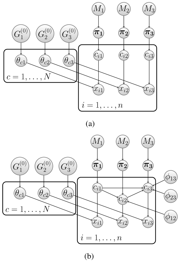
Figure 1: Graphical representation of $K=3$ DMA mixture models. (a) Independent case. (b) Modelling dependence between the latent component allocation variables (the MDI model). Figure from Kirk et al. (2012)

3 Model

We further develop the Multiple Data Integration (MDI) method of Kirk et al. (2012). MDI can be regarded as an extension of nonparametric Bayesian clustering methods to analyse simultaneously multiple data types, inferring the degree of similarity between the clustering structure in the data types. MDI hence produces clustering partitions for each data type, as well as an overall consensus clustering partition.

We note that another particular strength of MDI is that it infers the posterior distribution over the number of clusters in each data type. Hence, we can infer the likely number of clusters, given the data. Many clustering algorithms do not provide a method for doing this, which is a major shortcoming.

3.1 The MDI model

We consider a multi-dimensional data set, consisting of $K$ distinct data types (for example, gene expression, copy number, methylation or microRNA expression). Each data type will contain measurements for the same set of items, so that for each items we have $K$ vectors of measurements. We note that in general the numbers of features for each data type will be different from one another, and can be arbitrarily so for the MDI model.

We model each data type using a finite approximation to a Dirichlet process mixture model (Ishwaran & Zarepour, 2002), known as a Dirichlet-Multinomial Allocation (DMA) mixture model (Green & Richardson, 2001). The $K$ DMA models are coupled by a set of $\phi$ parameters that allow for information-sharing between the data types and provide a measurement of the level of similarity between pairs of types. Figure 1 shows a graphical representation of the MDI model.

The DMA mixture model for a single data type is given by the following equation.

$$p(x)=\sum_{c=1}^{N}\pi_{c}f(x|\theta_{c}).$$ (1)

Where $\pi_{c}$ are the mixture proportions, $f$ is a parametric density (such as a Gaussian) that models the $c$-th data type, and $\theta_{c}$ are the parameters associated with the $c$-th component. $N$ is the maximum number of mixture components, which is set typically to be large enough so as to not impact on the inference. When $N$ is large in this way, the behaviour of the DMA model approaches that of a Dirichlet process. To ensure this and as a tradeoff with computational cost, $N=\lceil n/2\rceil$ throughout this paper.

We note that different choices for the density $f$ allow us to model different types of data (for example, a normal distribution might be appropriate for continuous data, while a multinomial might be appropriate for categorical data). This imparts great flexibility to the MDI model.

Given observed data $x_{1},\ldots,x_{n}$, we wish to perform Bayesian inference for the unknown parameters in this model. We introduce latent component allocation variables $c_{j}\in\{1,\ldots,N\}$, such that $c_{i}$ is the component responsible for observation $x_{i}$. We then specify the model as follows:

$$x_{i}|c_{i},\boldsymbol{\theta} \sim F(\theta_{c_{i}}),$$

$$c_{i}|\boldsymbol{\pi} \sim\mbox{Multinomial}(\pi_{1},\ldots,\pi_{N}),$$

$$\pi_{1},\ldots,\pi_{N} \sim\mbox{Dirichlet}(\alpha/N,\ldots,\alpha/N),$$ (2)

$$\theta_{c} \sim G^{(0)},$$

where $F$ is the distribution corresponding to density $f$, $\boldsymbol{\pi}=(\pi_{1},\ldots,\pi_{N})$ is the collection of $N$ mixture proportions, $\alpha$ is a mass/concentration parameter (which may also be inferred), and $G^{(0)}$ is the prior for the component parameters.

Now considering the full MDI model with $K$ distinct data types, to couple the $K$ mixture models, the following conditional prior is introduced for the component allocation variables.

$$p(c_{i1},\dots,c_{iK}|\boldsymbol{\phi})\propto\prod_{k=1}^{K}\pi_{c_{ik}k}\prod_{k=1}^{K-1}\prod_{\ell=k+1}^{K}\left(1+\phi_{k\ell}{\mathbb{I}(c_{ik}=c_{i\ell})}\right),$$ (3)

where $\mathbb{I}$ is the indicator function, $\phi_{k\ell}\in\mathbb{R}_{\geq 0}$ is a parameter that controls the strength of association between datasets $k$ and $\ell$, and $\boldsymbol{\phi}$ is the collection of all $K(K-1)/2$ of the $\phi_{k\ell}$’s. $c_{ik}\in\{1,\ldots,N\}$ is the component allocation variable associated with item $i$ in model $k$, and $\pi_{c_{ik}k}$ is the mixture proportion associated with component $c_{ik}$ in model $k$. Informally, the larger $\phi_{k\ell}$, the more likely it is that $c_{ik}$ and $c_{i\ell}$ will take the same value, and hence the greater the degree of similarity between the clustering structure of dataset $k$ and dataset $\ell$. If all $\phi_{k\ell}=0$, then we recover the case of $K$ independent DMA mixture models (Figure 1b). We constrain the $\phi_{k\ell}$ to be non-negative.

We note that the $x_{ij}$ are assumed to be independent, given the clustering in MDI. The model then concentrates on modeling the joint distribution of the allocation variables $c_{i1},...,c_{iK}$ which induces correlation over the x’s.

3.2 Data Models

For the analyses in this paper, we use two different densities, $f_{Gaussian}$ and $f_{multinomial}$. These are respectively used for real-valued and discrete data and make reasonable assumptions (for the data used in this paper) about the expected noise characteristics.

For both data models, we assume that the features represent repeated, independent measurements of the underlying clustering partition. We therefore have the following equation.

$$f=\prod_{a}f_{a}$$ (4)

For the Gaussian density, we assume that each feature is modeled by a Gaussian likelihood of unknown mean and precision, subject to a Normal-Gamma prior. There density is therefore closed form and we hence marginalise the mean and precision.

We therefore have the following (marginal) likelihood function for the Gaussian case.

$$f_{a,Gaussian}=\frac{\Gamma(\alpha_{n})}{\Gamma(\alpha_{0})}\frac{\beta_{0}^{\alpha_{0}}}{\beta_{n}^{\alpha_{n}}}(\frac{\kappa_{0}}{\kappa_{n}})^{\frac{1}{2}}(2\pi)^{-\frac{n}{2}}$$ (5)

Where

$$\mu \sim N(0,(\kappa_{0}\lambda)^{-1})$$ (6)

$$\lambda \sim Ga(\alpha_{0},\beta_{0})$$ (7)

$$\kappa_{n} = \kappa_{0}+n$$ (8)

$$\alpha_{n} = \alpha_{0}+\frac{n}{2}$$ (9)

$$\beta_{n} = \beta_{0}+\frac{1}{2}\sum_{i=1}^{n}(x-\bar{x})^{2}+\frac{\kappa_{0}n\bar{x}^{2}}{2\kappa_{n}}$$ (10)

We set the Normal-Gamma hyperparameters to $\alpha_{0}=2$, $\beta_{0}=0.5$ and $\kappa_{0}=0.001$.

For the multinomial density, we assume that each feature is modeled by a multinomial likelihood, subject to a Dirichlet prior. The parameters of the multinomial likelihood are unknown, but because of the conjugate prior the density has a closed form and those parameters can hence be marginalised, leaving only the hyperparameters $\beta_{rq}$ to be defined.

We therefore have the following (marginal) likelihood function for the multinomial case.

$$f_{a,multinomial}=\prod_{q=1}^{Q}\frac{\Gamma(B_{q})}{\Gamma(S_{q}+B_{q})}\prod_{r=1}^{R}\frac{\Gamma(x_{rq}+\beta_{rq})}{\Gamma(\beta_{rq})}$$ (11)

We set the Dirichlet prior hyperparameters to $\beta_{rq}=0.5$.

3.3 Feature Selection

Because of the potentially large number of features in the various omic data types, we extend the Gaussian and multinomial data models to include feature selection. To do this, we include binary indicator parameters $I_{a}$ for each feature in a given data type. This modifies Equation 4 to the following:

$$f=\prod_{a}(I_{a}f_{a})+(1-I_{a})f_{a,null}$$ (12)

The factor for each feature will therefore either be $f_{a}$ or $f_{a,null}$. The $f_{a}$ are as before, so if all $I_{a}=1$ then we have the model with no feature selection.

The $f_{a,null}$ represent the alternative model that the feature is uninformative and hence all items are modeled as belonging to a single mixture component. We also make an approximation that the likelihood parameters are known, rather than marginalised over. This makes only a modest correction to the typical marginal likelihood values, but significantly speeds up the computation of the conditional distributions for Gibbs resampling.

For data models taking the form in Equation 4, we note that the distributions for Gibbs resampling of the $I_{a}$ are conditionally independent, given the $c_{ik}$. As MDI is written in Matlab, this allows us to vectorise the computation of the conditional distributions for the Gibbs resampling of all the $I_{a}$. This vectorisation makes the feature selection in MDI highly computationally efficient and fast to execute.

3.4 Split-Merge MCMC sampling

One characteristic of Gibbs samplers for mixture model clustering algorithms is that the MCMC chains can be relatively slow to mix. We have noticed this in particular for the number of occupied components.

To improve this, we have implemented a version of the sequential split-merge MCMC sampler of Dahl (2005). The split-merge steps are applied separately to each of the $K$ DMA models. These MCMC steps are proposed in addition to all the usual Gibbs steps described in Kirk et al. (2012). The increase in computation required for the split-merge steps is minor, and we find that while the acceptance rate for the steps is low, the overall effect is to substantially improve the mixing rate for the number of clusters for each data type.

3.5 Extraction of Clustering Partitions

We adopt a different approach to that of Kirk et al. (2012) to the extraction of clustering partitions from the posterior similarity matrix. Because the previously-used method (Fritsch & Ickstadt, 2009) is only available as an R package, for convenience we implement as part of the MDI code a simpler method based on a hierarchical clustering using the posterior similarity matrix. We note that the results in Fritsch & Ickstadt (2009) show that this approach produces similar performance to the previously-used method.

Using as distances (1 - posterior similarity), we perform standard hierarchical clustering with complete linkage. We set the number of clusters to be the MAP estimate of the number of clusters, taken from the MCMC analysis.

The resulting clustering partition should be regarded as a convenient summary of the full results. We would strongly encourage users of this method to not neglect other outputs such as the posterior similarity and fusion matrices.

Table 1: Bonferroni-corrected p-values for subtype Kaplan-Meier survival curves (nTests=20) For a given clinical outcome and data type/s, the Kaplan-Meier curves for each disease subtype are produced. P-values are computed using the log-rank test and considering the null hypothesis that all curves in a given set are drawn from the same underlying distribution.

data type/s	died	new event	progression	recurrence
all	1	0.66	0.11	$3.6\times 10^{-4}$
copy number	1	1	1	1
gene expression	$1.5\times 10^{-3}$	1	1	1
methylation	1	0.28	1	$2.0\times 10^{-3}$
microRNA	1	1	1	1

4 Results

We analyse gene expression, copy number variation, micro-RNA and methylation data for 277 glioblastoma patients using MDI. We identify a range of distinct disease subtypes and results, the most interesting of which we now describe.

Complete results can be found at https://sites.google.com/site/multipledatafusion/

We consider 5 distinct cases of summarising clustering partition (for each individual type, and also the consensus of all 4). For these we consider 4 binary, right-censored clinical outcomes: death, new tumour event, tumour progression, tumour recurrence. This gives us 20 cases in all.

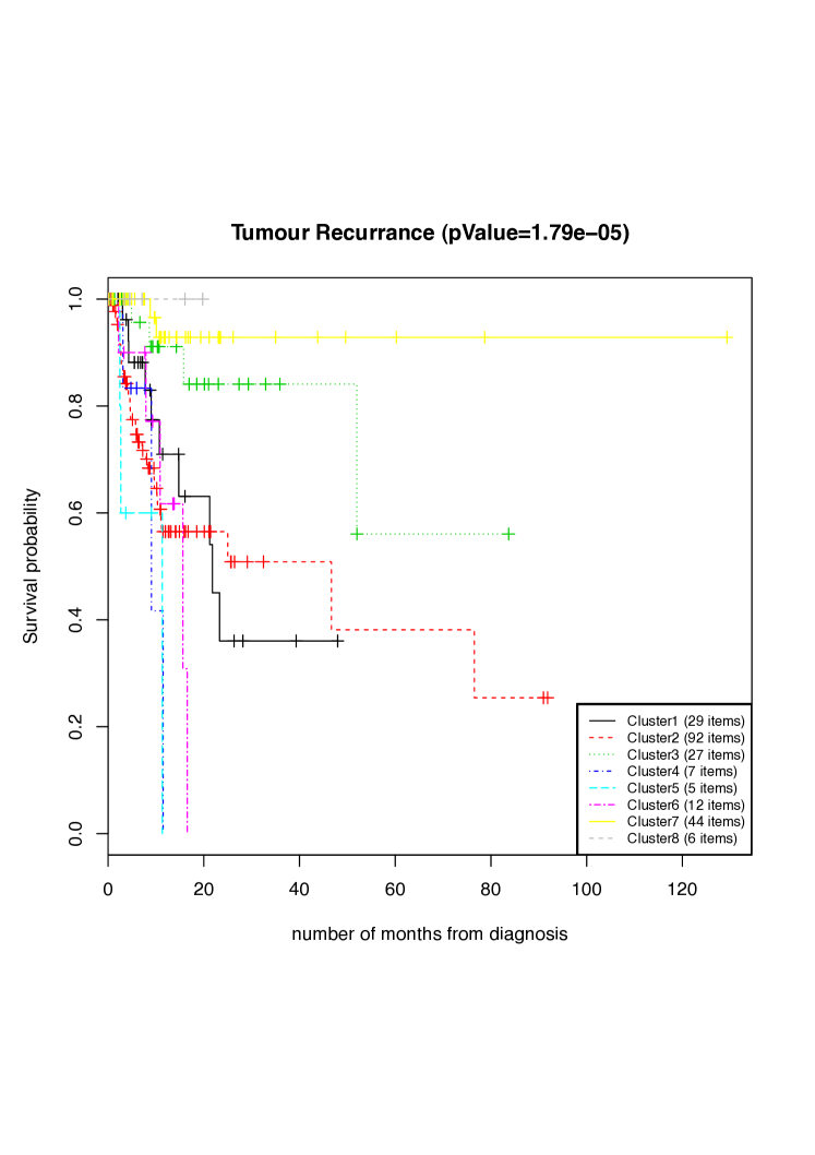
Figure 4: Kaplan-Meier survival curves plotting tumour recurrence for the consensus disease subtypes. The p-value is computed using a log-rank test. When quoted in Table 1, a Bonferroni correction has been applied to account for multiple hypothesis tests.

For each case, we plot the Kaplan-Meier survival curves for the set of disease subtypes. Table 1 shows the log-rank p-values for these plots, after application of a Bonferroni correction for multiple hypothesis testing (nTests=20). Examples of these plots can be seen in Figure 4. We note that in all cases we only consider subtypes containing at least 5 items and we only consider items for which there is clinical outcome information.

4.1 Consensus subtypes are prognostic for tumour recurrence

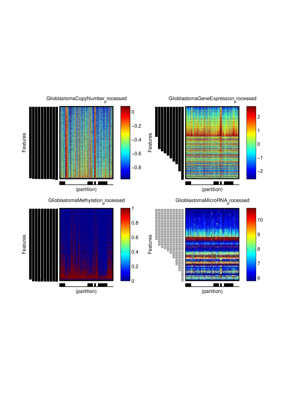
Figure 7: Plot of the 4 data types. The x-axis gives the data items (patients/tumour samples), sorted by the consensus clustering partition. The y-axis gives the selected features for each data type, with the dashed lines on the LHS indicating P(selected) for each feature. We note that any feature with P(selected)$<$0.1 is excluded from this plot, and also that the outlying 5% of pixels in each data type are clipped for the purposes of plotting.

We note that the consensus subtypes in general are strongly prognostic for tumour recurrence (log-rank p-value of $3.6\times 10^{-4}$ after correction for multiple hypothesis tests) (see Figure 7). Because the methylation status is measured at the point of diagnosis, this prognostic capability is predictive.

4.2 Interesting low-methylation subtype

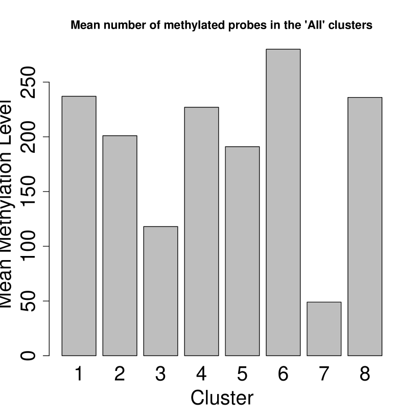
Figure 6: The mean number of methylated sites in each consensus subtype (out of a possible 769). A site is counted as methylated if it has been binarised to have unit value in the input methylation data in this analysis.

Consensus subtype 7 has particularly interesting characteristics. Comprising 47 items, it shows only very low levels of tumour recurrence (see Figure 4) and no new tumour events. All items in this subtype show very low relative levels of methylation (see Figure 6). This subtype contains 23 women and 24 men, with a median age of 53 and an age range of 14 to 81.

4.3 Gene expression subtypes are prognostic for survival outcome

Figure 5 shows the Kaplan-Meier survival curves for the 8 gene expression (GE) subtypes identified by MDI. These subtypes are prognostic for survival outcome (log-rank p-value of $1.5\times 10^{-3}$ after correction for multiple hypothesis tests).

This result is largely driven by GE cluster 7, which consists of 6 patients with particularly poor survival outcome (see Figure 5). Of these 6 patients, 3 die within 6 months of diagnosis, and the other 3 are omitted from the survival analysis as we do not have information on their survival or otherwise (they are missing data). As such, this result relies on a small number of patients and should therefore be treated with caution. However, further study is certainly warranted in case this subtype remains distinct with a larger number of members.

4.4 Partial overlap of clustering structure for different data types

The fusion matrix (Figure 2 ) and consensus clustering results show that there is a level of consistency in the clustering structure across the gene expression, copy number variation, methylation and microRNA data. However, inspection of the clustering partitions for each data type show that there are also differences in structure between each type. This indicates that a single clustering partition is not sufficient to capture all of the structure contained in the 4 data types.

4.5 Evidence for a biologically distinct glioblastoma subtype

Consensus cluster 5 consists of 8 patients and is noteworthy for highly distinctive data signatures in gene expression (over-expression), copy number (excess copies) and micro-RNA (over-expression in a subset of selected features).

This subtype is poor for tumour recurrence, and we suggest that the striking data signatures are suggestive of a distinctive set of biological mechanisms driving this tumour subtype.

4.6 Fusion matrix makes biological sense

The $\phi_{k\ell}$ parameters provide information on the level of agreement about clustering structure between pairs of data types. Figure 2 shows the posterior mean values for the $\phi_{k\ell}$. The principal sharing of structure is shown to be between gene expression and the other three data types, while other pairs of data types are less strongly related. This confirms what would be expected from prior knowledge of the underlying biological mechanisms. This is an important sanity check of the analysis, and shows that there is useful biological information in the data set.

4.7 MCMC details

The results presented in this paper are the result of 25 MCMC chains, each of $\approx 70,000$ samples. We sparse-sample the chains by a factor of 10 and remove the first 25% of each chain as burn-in. We check for adequate convergence by visual inspection of the MCMC time-series and histograms for each chain, overlaid on one another.

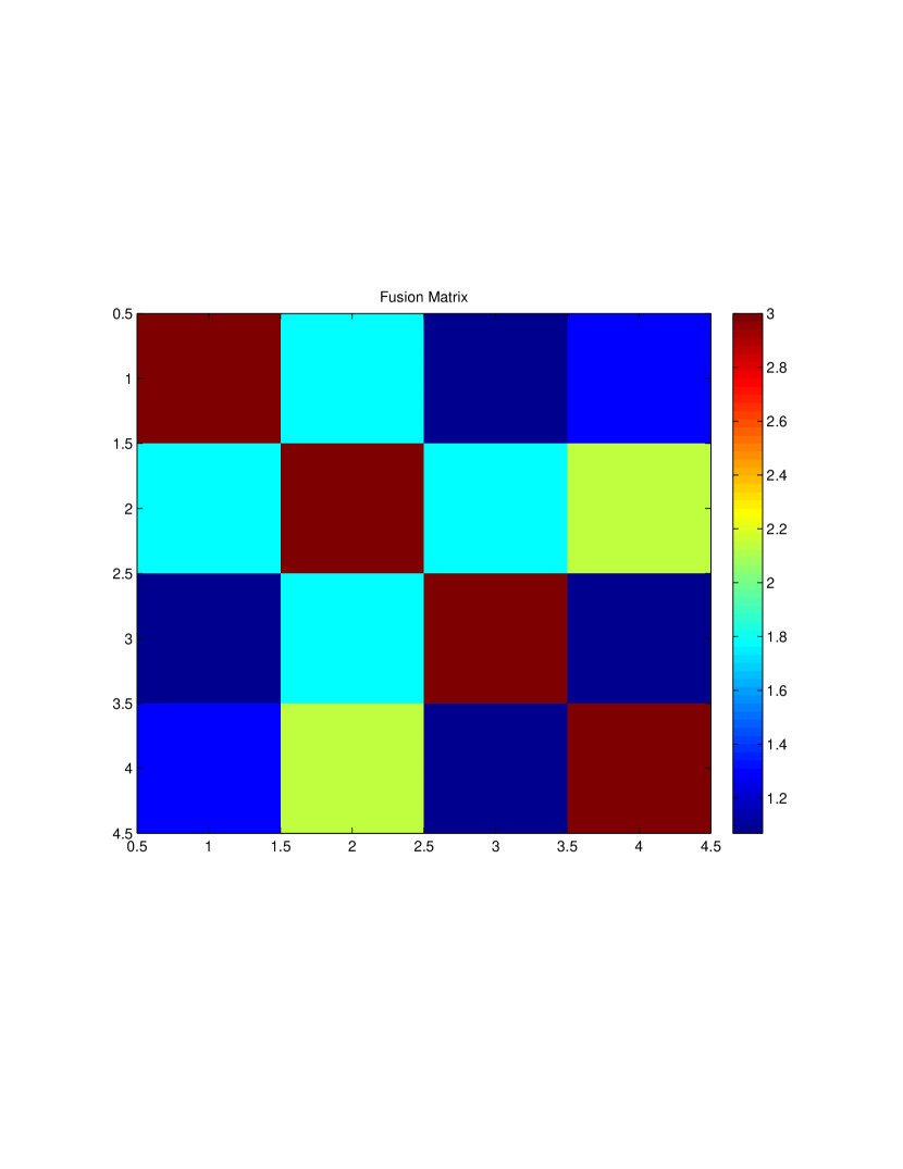
Figure 2: Matrix showing the posterior mean values for the $\phi_{k\ell}$. Shown are the copy number data (row 1), gene expression (row 2), methylation (row 3), microRNA (row 4). We note that the diagonal elements are undefined for the MDI model and so are set to arbitrary values so as to make the colour table convenient.

5 Conclusions

Figure 3: Posterior similarity matrix for the 277 data items. This matrix gives the posterior probability of given pairs of items belonging to the same cluster, averaged over the 4 data types. This is used to produce the consensus clustering partition. The matrix shown here has been sorted by the resulting partition, to better show the structure. The x-axis is labelled by alternating sets of bars/dots, denoting the different clusters. The LHS y-axis bars show the relative probability that a given item has the same cluster label across data types.

We have presented extensions to the MDI method that make it suitable for analysing multi-dimensional molecular cancer data sets. Using MDI to analyse the TCGA glioblastoma data, we have identified a number of important points.

• Both the 8 methylation and 8 data-consensus disease subtypes we have identified are significantly prognostic of tumour recurrence

• The 8 gene expression disease subtypes we have identified are significantly prognostic of survlval outcome

• We have identified a strongly prognostic glioblastoma subtype, noteworthy for its low levels of tumour recurrence methylation

• We have identified a small subtype of 6 patients based on gene expression for which there is very poor survival outcome, and postulate that this may identify a rare and agressive form of glioblastoma

• We have also identified a subtype of 8 patients with a highly distinctive data signature. This subtype has poor tumour recurrence, and it may represent a subtype whose underlying biology is highly distinctive, which may allow for more targetted therapy

• We note that the clustering structures for the 4 different data types overlap partially, but there is significantly more structure than can be explained by a single partition

Modern, large-scale cancer data sets contain a wealth of data types measuring the effects of genomic and environmental processes. We have demonstrated the effectiveness of combining these data types into a single analysis, and shown that the richness of structure contained by such multi-dimensional data sets necessitates statistical methods capable of capturing that richness.

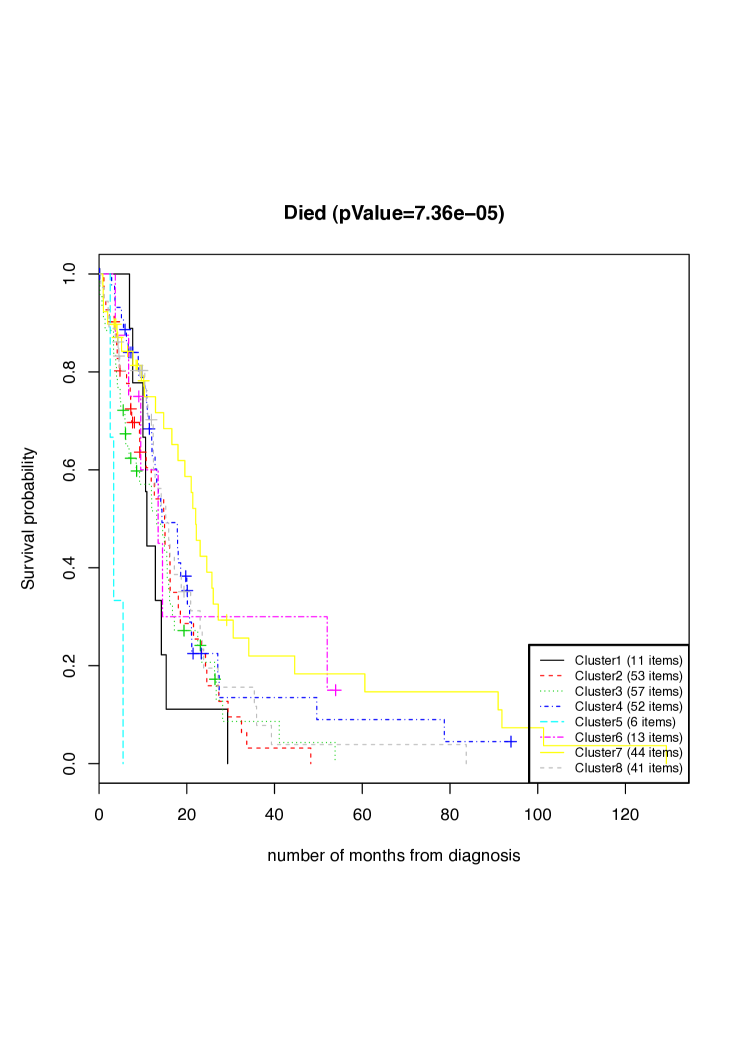
Figure 5: Kaplan-Meier survival curves for the gene expression disease subtypes. The p-value is computed using a log-rank test. When quoted in Table 1, a Bonferroni correction has been applied to account for multiple hypothesis tests.

Figure 8:

Figure 9:

Figure 10:

Figure 11:

References

- ACS (2011) ACS. Global cancer facts and figures 2nd edition. American Cancer Society, 2011.
- Antoniak (1974) Antoniak, C.E. Mixtures of Dirichlet processes with applications to Bayesian nonparametric problems. Annals of Statistics, 2:1152–1174, 1974.
- Curtis et al. (2012) Curtis, C. et al. The genomic and transcriptomic architecture of 2,000 breast tumours reveals novel subgroups. Nature, 2012.
- Dahl (2005) Dahl, D.B. Sequentially-allocated merge-split sampler for conjugate and nonconjugate dirichlet process mixture models. Journal of Computational and Graphical Statistics, 2005.
- Dahl (2006) Dahl, DB. Model-based clustering for expression data via a Dirichlet process mixture model. In Do, Kim-Anh, Müller, Peter, and Vannucci, Marina (eds.), Bayesian Inference for Gene Expression and Proteomics. Cambridge University Press, Cambridge, 2006.
- Escobar & West (1995) Escobar, Michael D. and West, Mike. Bayesian density estimation and inference using mixtures. Journal of the American Statistical Association, 90(430):577–588, 1995.
- Ferguson (1973) Ferguson, TS. A Bayesian analysis of some nonparametric problems. The Annals of Statistics, 1:209Ж230., 1973.
- Fritsch & Ickstadt (2009) Fritsch, Arno and Ickstadt, Katja. Improved criteria for clustering based on the posterior similarity matrix. Bayesian Anal, 4(2):367–391, 2009.
- Green & Richardson (2001) Green, PJ and Richardson, S. Modelling heterogeneity with and without the Dirichlet process. Scand J Stat, 28(2):355–375, Jan 2001.
- (10) http://cancergenome.nih.gov/. The cancer genome atlas.
- ICGC (2010) ICGC. International network of cancer genome projects. Nature, 464:993–998, 2010.
- Ishwaran & Zarepour (2002) Ishwaran, H and Zarepour, M. Exact and approximate representations for the sum Dirichlet process. Can J Stat, 30(2):269–283, 2002.
- Jemal et al. (2011) Jemal, A., Bray, F., Center, M.M., Ferlay, J., Ward, E., and Forman, D. Global cancer statistics. CA: a cancer journal for clinicians, 61(2):69–90, 2011.
- Kirk et al. (2012) Kirk, P., Griffin, J., Savage, R.S., Ghahramani, G., and Wild, D.L. Bayesian integration of multiple datasets. submitted, 2012.
- Rasmussen et al. (2007) Rasmussen, C., de la Cruz, B., Ghahramani, Z., and Wild, D. L. Modeling and visualizing uncertainty in gene expression clusters using Dirichlet process mixtures. IEEE/ACM Transactions on Computational Biology and Bioinformatics, 2007.
- Savage et al. (2010) Savage, R S, , Ghahramani, Z, Griffin, J E, de la Cruz, B, and Wild, D L. Discovering transcriptional modules by bayesian data integration. Bioinformatics, 26:158–167, 2010.
- Shen et al. (2009) Shen, R., Olshen, A.B., and Ladanyi, M. Integrative clustering of multiple genomic data types using a joint latent variable model with application to breast and lung cancer subtype analysis. Bioinformatics, 25(22):2906–12, Nov 2009.
- Stratton et al. (2009) Stratton, M.R., Campbell, P.J., and Futreal, A. The cancer genome. Nature, 458:719–724, 2009.
- TCGA (2008) TCGA. Comprehensive genomic characterization defines human glioblastoma genes and core pathways. Nature, 455:1061–1068, 2008.
- Yuan et al. (2011) Yuan, Y., Savage, R.S., and Markowetz, F. Patient-specific data fusion defines prognostic cancer subtypes. PLoS Comput Biol, 7(10):e1002227, Oct 2011.