A NEW RESULT ON THE ORIGIN OF THE EXTRAGALACTIC GAMMA-RAY BACKGROUND

Abstract

In the paper, we continually use the method of image stacking to study the origin of the extragalactic gamma-ray background (EGB) at GeV bands, and find that the Faint Images of the Radio Sky at Twenty centimeters (FIRST) sources undetected by the Large Area Telescope on the Fermi Gamma-ray Space Telescope can contribute about (56$\pm$6) % of the EGB. Because the FIRST is a flux limited sample of radio sources with incompleteness at the faint limit, we consider that the point-sources, including blazars, non-blazar AGNs, starburst galaxies, could produce a much larger fraction of the EGB.

1 Introduction

The extragalactic gamma-ray background (EGB) at GeV bands was first detected by the satellite Small Astronomy Satellite-2 (SAS-2; Fichtel et al., 1975), and its spectrum was measured with good accuracy by Fermi (also called isotropic diffuse background; Abdo et al., 2010f). Based on the first-year Fermi data, the EGB has been found to be consistent with a featureless power law with a photon index of $\sim$2.4 in the 0.2–100 GeV energy range and an integrated flux (E$\geq$100 MeV) of 1.03$\times 10^{-5}$ photon cm^-2 s^-1 sr^-1. The integrated flux with E$\geq$1 GeV is 4$\times 10^{-7}$ photon cm^-2 s^-1 sr^-1 (see Abdo et al., 2010c).

The origin of the EGB is one of the fundamental unsolved problems in astrophysics (see Kneiske, 2008, for a review). The EGB could originate from either truly diffuse processes or from unresolved point sources. Truly diffuse emission can arise from some processes such as the annihilation of dark matter (Ahn et al., 2007; Cuoco et al., 2010; Belikov & Hooper, 2010), the emission of high energy particles accelerated by intergalactic shocks which are produced during large scale structure formation (Gabici & Blasii,, 2003) etc.

Blazars, including BL Lac objects, flat spectrum radio quasars, or unidentified flat spectrum radio sources, represent the most numerous population detected by the Energetic Gamma Ray Experiment Telescope (EGRET) on the Compton Gamma Ray Observatory (Hartman et al., 1999) and by the Fermi-LAT (Abdo et al., 2010b; Ackermann et al., 2011). Therefore, blazars undetected by the EGRET or Fermi-LAT are the most likely candidates for the emission of the EGB. Many authors have studied the luminosity function of blazars and showed that the contribution of undetected blazars to the EGB could be in the range from 20 % to 100 % (Stecker & Salamon, 1996; Narumoto & Totani, 2006; Dermer, 2007; Cao & Bai, 2008; Kneiske & Mannheim, 2008; Inoue & Totani, 2009; Li & Cao, 2011; Malyshev & Hogg, 2011; Stecker & Venters, 2011). However, Abdo et al. (2010c) built a source count distribution at GeV bands and yielded that blazars undetected by the LAT can contribute about 23 % of the EGB. They ruled out blazars producing a large fraction of the EGB.

Non-blazar radio loud active galactic nuclei (AGNs) can also contribute a fraction to the EGB (Bhattacharya et al., 2009; Inoue, 2011), since some of them have been found to be $\gamma$-ray sources (Abdo et al., 2010d) and they outnumber blazars.

Starburst galaxies, which have intense star-formation, are expected to have high supernova (SN) rates. SN remnants are believed to accelerate primary cosmic rays (CRs) protons and electrons. The high SN rates in starburst galaxies imply high CR emissivity. When high energy CR protons collide with interstellar medium (ISM) nucleons, they create pions decaying into secondary electrons and positrons, $\gamma$-rays, and neutrinos. Ackermann et al. (2012a) have found quasi-linear scaling relations between $\gamma$-ray luminosity and both radio continuum luminosity and total infrared luminosity. To data, several starburst galaxies have been detected by the Fermi-LAT (Abdo et al., 2010a; Nolan et al., 2012; Ackermann et al., 2012a). Therefore, starbursts can also contribute a fraction of the EGB (Thompson et al., 2007; Bhattacharya & Sreekumar, 2009; Lacki et al., 2011; Makiya et al., 2011).

Nevertheless, normal galaxies (Bhattacharya & Sreekumar, 2009; Fields et al., 2010) or radio-quiet AGNs (Inoue et al., 2008; Inoue & Totani, 2009) can also contribute a fraction of the EGB.

We introduced a new method of image stacking to directly study the undetected but possible $\gamma$-ray point sources (Zhou et al., 2011). Applying the method to the Australia Telescope 20 GHz Survey (AT20G; Murphy et al., 2010) sources undetected by the LAT, we found that these sources contribute about 10.5 % of the EGB in the 1–3 GeV energy ranges.

In this paper, we continually use the method to study the origin of the EGB, and find that the FIRST sources undetected by the LAT can contribute about (56$\pm$6) % of the EGB. We also discuss the implications.

2 FIRST

The Faint Images of the Radio Sky at Twenty centimeters (FIRST; Becker et al., 1995) program is using the Very Large Array (VLA) to produce a map of the 20 cm (1.4 GHz) sky with a beam size of 5.^′′4 and an rms sensitivity of about 0.15 mJy beam^-1. The accuracy of source position is better than 1^′′. The survey has covered an area of about 9,055 deg² in the north Galactic cap and a smaller area along the celestial equator, corresponding to the sky regions observed by the Sloan Digital Sky Survey (SDSS). At the 1 mJy source detection threshold, the source surface density is $\sim$ 90 deg^-2, and the catalog includes $\sim 8\times 10^{5}$ sources, in which about 30% of them have counterparts in the SDSS (Ivezić et al., 2002).

The FIRST catalog lists two types of 20 cm continuum flux density, e.g. the peak value, $F_{\rm peak}$, and the integrated flux density, $F_{\rm int}$. These measurements are derived from two-dimensional Gaussian fitting for each source, where the source maps are generated from the co-added images from 12 pointings.

Ivezić et al. (2002) found that about 30 % of FIRST sources was positional association within 1.^′′5 with an SDSS source in 1230 deg² of sky. The majority (83 %) of the FIRST sources identified with an SDSS source brighter than $r^{*}$ = 21 are optically resolved. About 30 % of them are radio galaxies in which emission-line ratios indicate AGNs; the others are starburst galaxies. Nearly all optically unresolved radio sources have nonstellar colors, indicating quasars. Because there is no significant difference in the radio properties between FIRST sources with and without optical identifications, the majority of unmatched FIRST sources could be too optically faint to be detected in SDSS images, and the fractions of quasars and galaxies are roughly the same for the two subsamples.

Because two subsamples of the FIRST catalog are $\gamma$-ray emitters, this catalog maybe a good tracer for the undetected $\gamma$-ray point sources.

3 Method

For a sample of possible $\gamma$-ray point sources undetected by the Fermi due to their faint fluxes, soft spectra (Abdo et al., 2010e) or the source confusion (Stecker & Venters, 2011), we can stack a large number of them to improve the statistics (White et al., 2007; Ando & Kusenko, 2010). We have used the Maximum Likelihood (ML) method to derive the fluxes of the stacked point sources (Zhou et al., 2011). But for a very large sample, this method is very time consuming. Therefore, in this paper, we use a rough but simple ML method to derive the fluxes.

The photons we used in our analysis are taken during the period of 2008 August 4 (15:43 UTC) – 2011 October 20 (23:33 UTC), about three years. During most of this time, Fermi was operated in sky-scanning survey mode (viewing direction rocking north and south of the zenith on alternate orbits). Time intervals flagged as ‘bad’ (a very small fraction) and the period of the rocking angle of the LAT greater than 52^∘ was excluded. Only the photons in the 1–100 GeV energy range with small 68 % containment radius (better than 1^∘) and little confusion (see Atwood et al., 2009; Abdo et al., 2009) are used. These photons are also needed to satisfy the standard low-background event selection (termed “Source” class events) corresponding to the P7V6 instrument response functions in the present analysis. The effect of Earth albedo backgrounds was greatly reduced by removing photons coming from zenith angles $<100^{\circ}$. In this procedure, the tools of gtselect and gtmktime are used.

Stacking the images of the sources, we collect all photons that are at most $1^{\circ}$ away from any source of our sample and then record their angular distance ($\theta_{i}$, in units of deg) between the photon and the source. The $1^{\circ}$ is enough despite some photons attributed to the central stacked point sources are not in the stacked image. Due to the faintness of the stacked point sources, in the outer of the stacked image, the signal of the stacked point sources is very weak.

In order to minimize the influence of strong point sources, the sources away from any second Fermi-LAT catalog (2FGL; Nolan et al., 2012) sources less $2^{\circ}$ ($3^{\circ}$ for 2GFL sources with fluxes larger than $10^{-9}$ photon cm^-2 s^-1 in the 1–100 GeV energy range) are not used. In order to minimize the influence of strong emission from the Galactic plane, only the sources locating at high Galactic latitudes, e.g. $|b|>15^{\circ}$, are used.

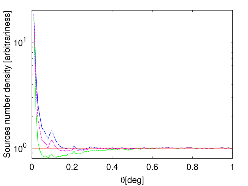
Figure 1: The normalized source number density profiles around the FIRST sources with $F_{\rm peak}\geq$100 mJy, for all sources by dot-dashed (blue) line, for the sources randomly removed with the probability of their P(S) by dotted (magenta) line, and for the sources with P(S)$<$0.1 by dashed (green) line. The solid (red) line represents the uniform density profile.

There are a small number of spurious sources that are sidelobes of nearby bright sources. In recent catalog, Becker et al. (2003) uesd P(S) to indicate the probability of that the source is spurious (most commonly because it is a sidelobe of a nearby bright source). The mean value of P(S) is 0.088, which indicates that about 8.8 % of the sources are sidelobes. They are concentrated around bright sources (see White et al., 1997, 2013, for detail), and should be removed first. In Figure 1 we show the number density of all FIRST sources and the sources having $P(S)\leq 0.1$ around the FIRST sources with $F_{\rm peak}\geq$100 mJy, respectively. A strict P(S) cutting, such as P(S)$\leq$0.1, is not appropriate. We randomly remove some sources with the probability of their P(S) except the sources with P(S)=0.014 (e.g., the minimum value of P(S), for about 72 % of all sources). This procedure does not try to remove sidelobes as much as possible, but to make the distribution of the rest sources around the bright sources as uniform as possible. The number density of the rest sources around the FIRST sources with $F_{\rm peak}\geq$100 mJy is also shown in Figure 1. The distribution is still not uniform enough, we will investigate the effect of uniform distribution in the following section.

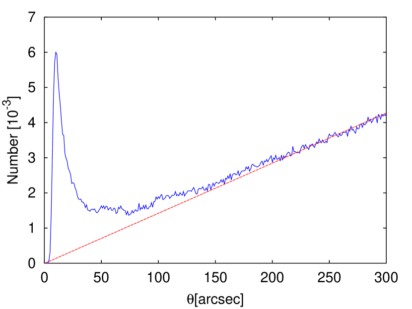
Figure 2: The mean number distribution of FIRST sources around one FIRST source. The dashed (red) line represents an estimate of the chance coincidence rate.

Many sources in the FIRST catalog are not independent objects but are components of a single object with complex morphology (White et al., 1997). In Figure 2, we show the mean source number distribution of other FIRST sources around one FIRST source. It is found that the possibility of finding another FIRST source near a FIRST source, especially closer than $\sim 50^{\prime\prime}$, is larger than one expected from a random source distribution. Therefore, when a group sources fall within 50^′′ of their nearest neighbors, we treat them as a single object. Nearly 30 % of the FIRST sources belongs to such sources. The cutoff of 50^′′ is a trade-off between the completeness and contamination of the sample. For a larger cutoff, more complex sources are merged, but more independent sources are also merged. The use of 50^′′ cutoff will produce small uncertainty introduced by the misclassified sources, and will be discussed in the following section.

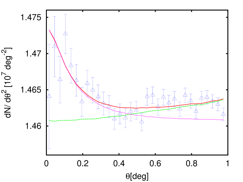
Figure 3: The photon number density profile of the stacked FIRST sources with $F_{\rm peak}\geq$1 mJy. The dashed (green) line represents the diffuse background, while the dotted (magenta) line represents the point source added by an arbitrary factor. The solid (red) line represents the best-fit model. The $\chi^{2}$ over degree of freedom (dof) is $\chi^{2}/{\rm dof}=30.7/31$, indicating that the model gives a satisfactory fit to the data. The TS is 43.0, corresponding to a significance of $\sim 6.7\sigma$.

The photon number density profile of the stacked image of FIRST sources with $F_{\rm peak}\geq$1 mJy is shown in Figure 3. It is shown that the center of the stacked image has higher photon number density and the stacked point source has nonzero flux.

We use $\sigma_{e}(\theta)$ to further prove the presence of the point source, which is the confidence level of stacked image representing photons within the radius of $\theta$ more than the expectation in the uniform density. It is defined as

$$\sigma_{e}(\theta)=\frac{N(\theta)-\frac{N}{\Theta^{2}}\theta^{2}}{\sqrt{\frac{N}{\Theta^{2}}\theta^{2}}},$$ (1)

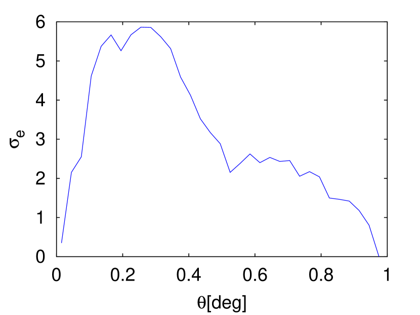
Figure 4: $\sigma_{e}(\theta)$ for the stacked image of the FIRST sources.

where $N(\theta)$ is the number of photons with $\theta_{i}<\theta$, $N$ is the number of photons with $\theta_{i}<\Theta$, here $\Theta=1^{\circ}$. The $\sigma_{e}(\theta)$ is presented in Figure 4. The excess of photons is very obvious within $\theta\sim 0.3^{\circ}$.

we apply the maximum likelihood (ML) method to derive the flux of the stacked point source. The likelihood is the probability of the observed data for a specific model. For our case, it is defined as

$$L=\prod_{i=1}^{33}p_{i},$$ (2)

where

$$p_{i}={\frac{1}{\sqrt{2\pi N_{i}}}\exp\left[-\frac{(N_{i}-M_{i})^{2}}{2N_{i}}\right]}$$ (3)

is the normal probability of observing $M_{i}$ counts in $i$-th bin when the number of counts predicted by model is $N_{i}$. The logarithm of the likelihood is conveniently calculated:

$$\ln L=\sum_{i=1}^{33}\left[-0.5\ln(2\pi)-0.5\ln N_{i}-\frac{(N_{i}-M_{i})^{2}}{2N_{i}}\right].$$ (4)

For simplicity, in our model there are only two components, e.g., the central stacked point source and diffuse background source, and

$$N_{i}=N_{s}n_{si}+N_{b}n_{bi},$$ (5)

$$N=N_{s}+N_{b},$$ (6)

where $N_{s}$ and $N_{b}$ are the photon numbers attributed to the central stacked point source and the diffuse background source, respectively. $n_{si}$ and $n_{bi}$ are the normalized photon number distributions of two class sources.

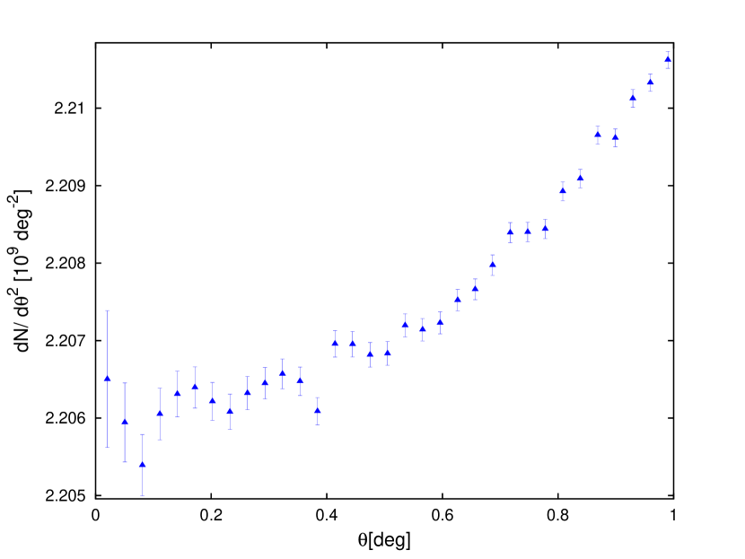
Figure 5: The photon number density profile of the stacked imaginary sources.

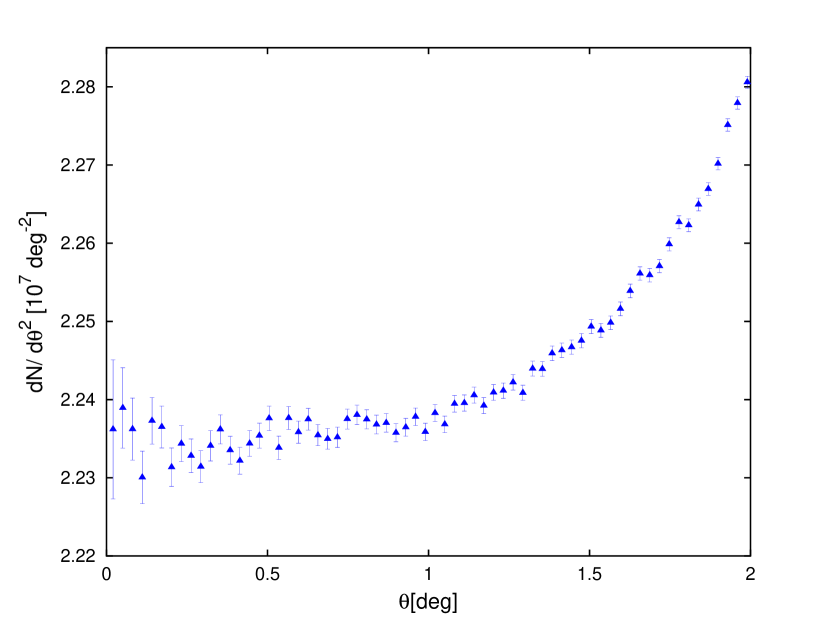
Figure 6: Same as Figure 5, but angular range is extended to 2^∘ and a small number of imaginary sources is stacked. In the figure, the effect of the nearby 2FGL sources is more obvious.

In order to determine $n_{bi}$, we stacked $10^{8}$ imaginary sources which is isotropically distributed on the sky. In fact, only $\sim 4\times 10^{7}$ sources far away strong sources are ultimately stacked. Because the sources we stacked here are not true $\gamma$-ray point sources, the stacked image only contains diffuse backgrounds. The photon number density profile of the stacked image is shown in Figure 5. It is found that the diffuse background is not uniform and has higher density in the outer of the stacked image, implying that the profile is affected by the 2FGL sources near the stacked image. In Figure 6 we show the photon number density profile of the stacked image which is extended to 2^∘, indicating that the effect of the nearby point sources is much obvious.

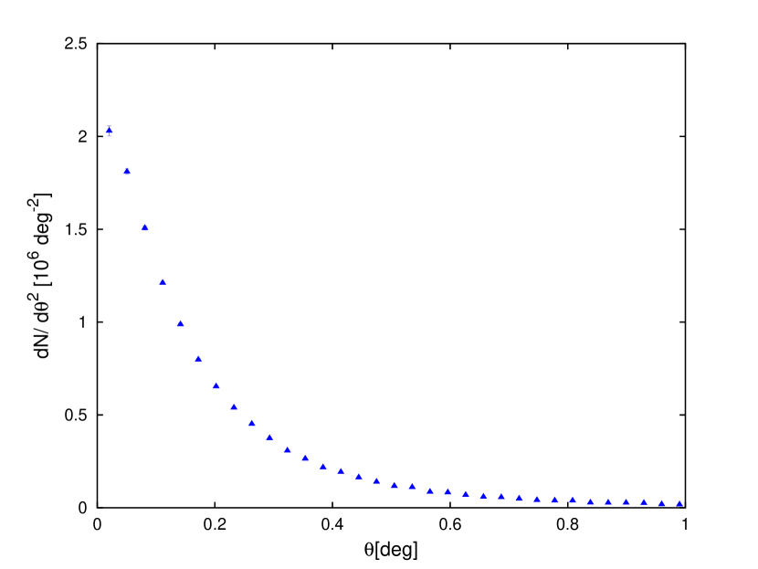
Figure 8: The photon number density profile of the simulated source with coordinates of (RA, DEC) = (190^∘, 30^∘ ).

In order to determine $n_{si}$, we simulate a source with a flux of $5\times 10^{-6}$ photon cm^-2 s^-1 in the 1–100 GeV energy range and the coordinate of (RA, DEC) = (190^∘, 30^∘). It has a power law spectrum and the photon index is 2.4, which is a typical value of the detected sources. The tool gtobssim has been used in this procedure. The photon number density profile of this source is shown in Figure 8.

We use the likelihood ratio to test the hypothesis. The point-source “test statistic” (TS) is defined as

$${\rm TS}=-2(\ln L_{0}-\ln L_{1})$$ (7)

where $L_{1}$ and $L_{0}$ are the likelihood with and without point source. The TS of each source is related to the probability of that such an excess is obtained from background fluctuations alone. The probability distribution in such a situation is not known precisely (Protassov et al., 2002). However, we only consider positive fluctuations, in which each fitting involves one degree of freedom, and according to Wilks’s theorem (Wilks, 1938) the probability with at least TS is close to that of the $\chi^{2}/2$ distribution with one degree of freedom. Therefore the detected significance of a point source is approximately $\sqrt{\rm TS}\sigma$ (see Mattox et al., 1996).

4 Result and Discussion

For the stacked point source of the FIRST sources with $F_{\rm peak}\geq$1 mJy, the estimated $N_{s}$ is $2.51\times 10^{4}$, in which its TS is 43.0, corresponding to a significance of $\sim 6.7\sigma$. The $\chi^{2}$ over degree of freedom (dof) is $\chi^{2}/{\rm dof}=30.7/31$, indicating that the model gives a satisfactory fit to the data.

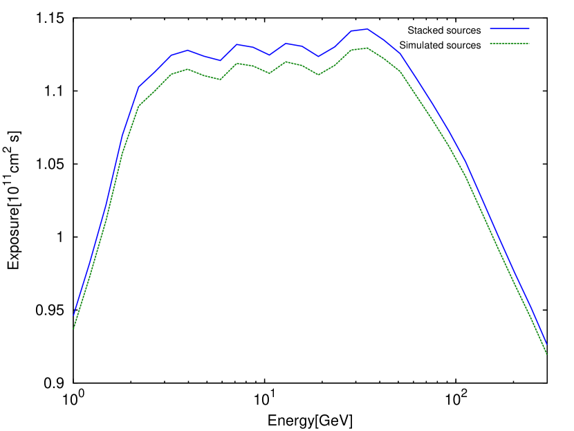
Figure 7: The exposures of the stacked source and the simulated source with coordinates of (RA, DEC) = (190^∘, 30^∘ ).

$N_{s}$ is proportional to the flux and exposure of the stacked point source. The exposure is the mean of the exposures of all stacked sources. But the calculation of the exposures for all stacked sources is very time consuming, and the exposure of all sky is relatively uniform, owing to the large field-of-view and the rocking-scanning pattern of the sky survey (Nolan et al., 2012), we use the mean exposure of about 1 % randomly selected FIRST sources to represent them. The exposures of the stacked point source and the simulated source are shown in Figure 7, which are roughly the same. The simulated source has a flux of $5\times 10^{-6}$ photon cm^-2 s^-1 and $\sim 4.1\times 10^{5}$ photons within $1^{\circ}$. The stacked point source has $\sim 2.51\times 10^{4}$ photons within $1^{\circ}$, corresponding to a flux of $\sim 3.09\times 10^{-7}$ photon cm^-2 s^-1. The FIRST covers an area of about 9055 deg², in which 321556 out of 640919 sources are stacked, indicating that the stacked point sources cover an area ( i.e. the area covered by the FIRST sample excluding all holes produced in the Fermi map by excluding photons in the vicinity of 2FGL sources.) of about 4543 deg². In this sky region the total flux of the EGB is $\sim 5.7\times 10^{-7}$ photon cm^-2 s^-1, implying that these sources can contribute $\sim 56\,\%$ of the EGB.

A decrease of 0.5 from its maximum value in $\ln L$ corresponds to 68 % confidence (1$\,\sigma$) region for the parameter (see Mattox et al., 1996). We use this variance to estimate the error of the flux and find that 1$\,\sigma$ error is $0.33\times 10^{-7}$ photon cm^-2 s^-1, implying that the FIRST sources contribute about (56$\pm$ 6) % of the EGB.

The effective area is an important factor of uncertainties. The current estimate of the remaining systematic uncertainty is 10 % at 100 MeV, decreasing to 5 % at 560 MeV and increasing to 10 % at 10 GeV and above (Ackermann et al., 2012b). This uncertainty is uniformly applied to all sources (Nolan et al., 2012). The error of the fraction of FIRST sources contributed to the EGB is much smaller.

In order to verify the effectiveness and accuracy of our method, we do the Monte Carlo simulation using the tool gtobssim. The simulating time is $\sim 10^{8}$ s, equaling the time of real data we used. We simulate $7.8\times 10^{5}$ point sources with fluxes of $10^{-12}$ photon cm^-2 s^-1 in the 1–100 GeV energy range. The flux distribution does not affect our results, which only depend on the total flux. They have power law spectra, in which the photon index of each source is drawn from a Gaussian distribution with a mean of 2.40 and $1\,\sigma$ width of 0.24, which is the same with the intrinsic distribution of photon indices (Abdo et al., 2010c). The coordinates of each source are randomly drawn to produce an isotropic distribution on the sky between right ascensions of 95^∘ and 270^∘, declinations of -10^∘ and +70^∘, which covers the main area observed by the FIRST survey. The simulated sources have similar source surface density with the FIRST sources, in which some sources are randomly removed according to the probability of their P(S) nd sources separated by less than 50^′′ are merged to a single source.

The simulated photons are isotropic in this area except edge part. We model the Galactic diffuse background using the models (gal_2yearp7v6_v0.fits) recommended by the LAT team, although it only contributes an uniform background to the stacked image. The EGB is not modeled, because the photons from point sources are actually regarded as the EGB.

To avoid the edge effect, we only stack the sources with the coordinates between right ascensions of 100^∘ and 265^∘, declinations of -5^∘ and +65^∘. Only about 2.2$\times 10^{5}$ of randomly selected simulated sources are stacked to obtain the similar flux with the stacked source of the FIRST sources. Other $\sim 1\times 10^{5}$ random positions are also stacked to obtain the similar photon number density with the stacked image of the FIRST sources. The photon number density profile of the stacked image is shown in Figure 9. Then we use the ML method to obtain the mean flux, which is 1.08$\times 10^{-12}$ photon cm^-2 s^-1. Its TS is 41.9, and $\chi^{2}$ is 31.7. The $1\,\sigma$ error is 1.5$\times 10^{-13}$  photon cm^-2 s^-1. Therefore, the derived mean flux is equal to the input flux within $1\,\sigma$ error, indicating that our flux estimation is correct and reliable.

The stacked image contains some regions which are not independent, leading to most photons being counted more than once. If a photon comes from other point source rather than the center source, it will be regarded as a part of the backgrounds and does not affect our results, as proved by the simulation.

In order to investigate the effect of the complex source merging and the sidelobe removing on our results, we use different $\theta_{cut}$ to merger the complex sources. The result, shown in Figure 10, presents that the fraction decreases when the $\theta_{cut}$ increases. This is due to two factors: (1) many sidelobes and complex sources are merged; (2) many independent sources are wrongly merged.

For more detail, we also merger the simulated sources using various $\theta_{cut}$ to calculate the total flux of the samples, in which the Galactic diffuse background is not added. The result is shown in Figure 10. The slope of the first curve is obviously steeper than that of the second curve when $\theta_{cut}\lesssim 100^{\prime\prime}$, but the slopes of two curves are nearly the same when $\theta_{cut}\gtrsim 100^{\prime\prime}$. This indicates that the effect of sidelobe and complex source merging is obvious only when $\theta_{cut}\lesssim 100^{\prime\prime}$. However, when $\theta_{cut}=50^{\prime\prime}$, the effect of the complex source merging and the sidelobes removing is small, and only makes the fraction to be overestimated by about 2 %. The wrong merging of independent sources makes the fraction to be also underestimated by about 2 %. Therefore, the cutoff of 50^′′ is appropriate and only introduces a small uncertainty.

Considering that the FIRST is a flux limited sample of radio sources and incomplete at the faint limit (White et al., 1997), we consider that when the sample is more complete or its radio flux limit further decreases, the contribution of the FIRST sources to the EGB should increases, but the exact fraction is not clear because it depends on the shape of the radio source count distribution below the FIRST flux limit and the correlation between the source radio and $\gamma$-ray luminosity. Nevertheless, normal galaxies (Bhattacharya & Sreekumar, 2009; Fields et al., 2010) or radio-quiet AGNs (Inoue et al., 2008; Inoue & Totani, 2009), which cannot be well traced by the FIRST survey (only a few fraction of those sources can be included in FIRST), can also contribute a fraction of the EGB, we think that the point sources can contribute most of the EGB.

5 Conclusions

In the paper, we use the method of image stacking to study the origin of the EGB, and find that the FIRST sources undetected by LAT can contribute about (56$\pm$6) % of the EGB. Considering the flux limit and incompleteness of the sample at the faint limit, we think that most of the EGB is distributed by point sources which are not resolved by LAT because of source confusion and weak flux. The main contributors of the EGB maybe blazars, non-blazars AGNs and starburst galaxies. But it is difficult to derive the exact fraction of each population contributing to the EGB using our method alone.

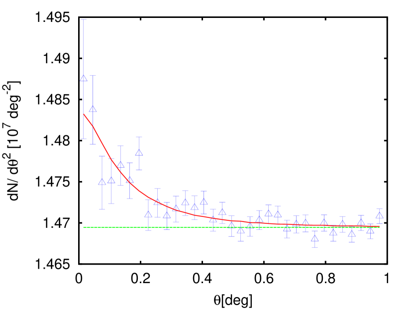
Figure 9: The photon number density profile of the stacked image using the simulated data. The dashed (green) line represents the diffuse background which is uniform. The solid (red) line represents the best-fit model, in which TS is 41.9, and $\chi^{2}$ is 31.7.

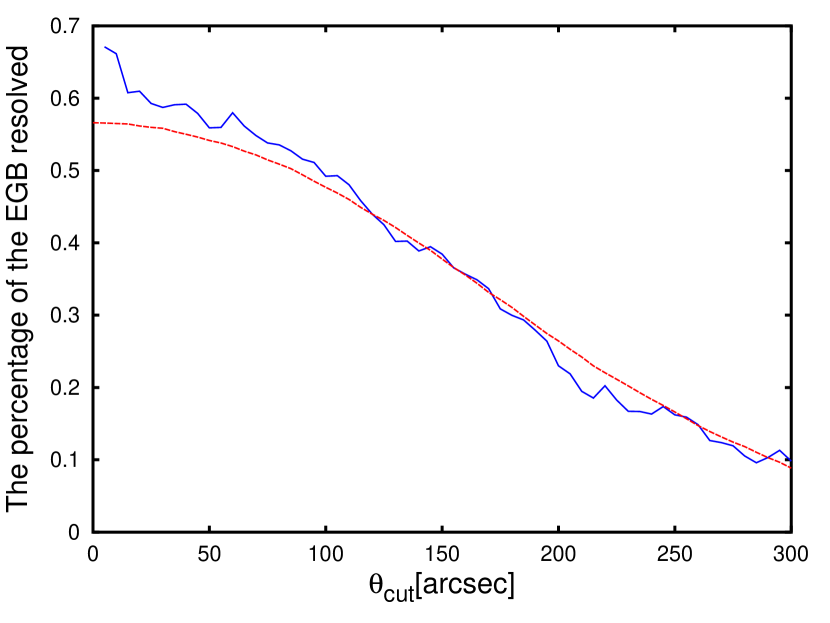
Figure 10: The percentage of the EGB resolved as a function of angular cut in the FIRST catalog. The dashed (red) line represent the expected dependence of the percentage on the angular cut for a random source distribution, which is obtained from the simulation. For comparison, two curves are normalized to have same value at $\theta_{cut}=120^{\prime\prime}$.

References

- Abdo et al. (2009) Abdo, A. A., et al. 2009, ApJS, 183, 46
- Abdo et al. (2010a) Abdo, A. A., et al. 2010a, ApJ, 709, L152
- Abdo et al. (2010b) Abdo, A. A., et al. 2010b, ApJ, 715, 429
- Abdo et al. (2010c) Abdo, A. A., et al. 2010c, ApJ, 720, 435
- Abdo et al. (2010d) Abdo, A. A., et al. 2010d, ApJ, 720, 912
- Abdo et al. (2010e) Abdo, A. A., et al. 2010e, ApJS, 188, 405
- Abdo et al. (2010f) Abdo, A. A., et al. 2010f, Physical Review Letters, 104, 101101
- Nolan et al. (2012) Nolan, P. L., et al. 2012, ApJS, 199, 31
- Ackermann et al. (2011) Ackermann, M., et al. 2011, ApJ, 743, 171
- Ackermann et al. (2012a) Ackermann, M., et al. 2012, ApJ, 755, 164
- Ackermann et al. (2012b) Ackermann, M., et al. 2012, ApJS, Accepted(arXiv:1206.1896)
- Ahn et al. (2007) Ahn, E. J., er al. 2007, Phys. Rev. D, 76, 023517
- Ando & Kusenko (2010) Ando, S., & Kusenko, A. 2010, ApJ, 2010, 722, L39
- Atwood et al. (2009) Atwood, W. B., et al. 2009, ApJ, 697, 1071
- Becker et al. (1995) Becker, R. H., White, R. L., & Helfand, D. J. 1995, ApJ, 4, 559
- Becker et al. (2003) Becker,R.H., Helfand, D. J., White,R. L., Gregg,M.D., & Laurent-Muehleisen, S. A. 2003, VizieR Online Data Catalog, 8071, 0
- Belikov & Hooper (2010) Belikov, A. V., & Hooper, D. 2010, Phys. Rev. D, 81, 043505
- Bhattacharya et al. (2009) Bhattacharya, D., Sreekumar, P., & Mukherjee, R. 2009, RAA, 9, 1205
- Bhattacharya & Sreekumar (2009) Bhattacharya, D., & Sreekumar, P. 2009, RAA, 9, 509
- Cao & Bai (2008) Cao, X. W., & Bai, J. M. 2008, ApJ, 673, L131
- Cuoco et al. (2010) Cuoco, A., Sellerholm, A., Conrad, J., & Hannestad, S. 2010, MNRAS, 414, 2040
- Dermer (2007) Dermer, C. D. 2007, ApJ, 659, 958
- Fichtel et al. (1975) Fichtel, C. E., et al. 1975, ApJ, 198, 163
- Fields et al. (2010) Fields, B. D., Pavlidou, V., Prodanović, T. 2010, ApJ, 722, L199
- Gabici & Blasii, (2003) Gabici, S., & Blasi, P. 2003, APh, 19, 679
- Hartman et al. (1999) Hartman, R. C., et al. 1999, ApJS, 123, 79
- Inoue (2011) Inoue, Y., 2011, ApJ, 733, 66
- Inoue & Totani (2009) Inoue, Y., & Totani T. 2009,ApJ, 702, 523
- Inoue et al. (2008) Inoue, Y., Totani, T., & Ueda, Y. 2008, ApJ, 672, L5
- Ivezić et al. (2002) Ivezić, Ž., et al. 2002, AJ, 124, 2364
- Kneiske (2008) Kneiske, T.M. 2008, ChJAS, 8, 219
- Kneiske & Mannheim (2008) Kneiske, T. M. & Mannheim, K. 2008, A&A, 479, 41
- Lacki et al. (2011) Lacki, B. C., et al. 2011, ApJ, 734, 107
- Li & Cao (2011) Li, F., & Cao, X. 2011, RAA, 11, 879
- Makiya et al. (2011) Makiya, Ryu., Totani, Tomonori., Kobayashi, Masakazu A. R. 2011, ApJ, 728, 158
- Malyshev & Hogg (2011) Dmitry, Malyshev., & David, W. Hogg. 2011, ApJ, 738, 181
- Mattox et al. (1996) Mattox, J. R., et al., 1996, ApJ, 461, 396
- Murphy et al. (2010) Murphy, T., at al. 2010, MNRAS, 2010, 402, 2403
- Narumoto & Totani (2006) Narumoto, T., & Totani, T. 2006, ApJ, 643, 81
- Protassov et al. (2002) Protassov, R., van Dyk, D. A., Connors, A., Kashyap, V. L., & Siemiginowska, A. 2002, ApJ, 571, 545
- Stecker & Salamon (1996) Stecker, F. W., & Salamon, M. H. 1996, ApJ, 464, 600
- Stecker & Venters (2011) Stecker, F. W., & Venters, T. M. 2011, ApJ, 736, 40
- Thompson et al. (2007) Thompson, T. A., Quataert, E., & Waxman, E. 2007, ApJ, 654, 219
- White et al. (2013) Whiter, R. L., et al., in preparation
- White et al. (2007) Whiter, R. L., et al., 2007, ApJ, 654, 99
- White et al. (1997) White, R. L., Becker, R. H., Helfand, D. J., & Gregg, M. D. 1997, ApJ, 475, 479
- Wilks (1938) Wilks, S. S. 1938, Ann. Math. Stat., 9, 60
- Zhou et al. (2011) Zhou, M., Wang, J. C., & Gao, X. Y. 2011, ApJ, 727, L46