Warped Alternatives to Froggatt-Nielsen Models

Abstract

We consider the Randall-Sundrum (RS) set-up to be a theory of flavour, as an alternative to Froggatt-Nielsen (FN) models instead of as a solution to the hierarchy problem. The RS framework is modified by taking the low energy brane to be at the GUT scale. This also alleviates constraints from flavour physics. Fermion masses and mixing angles are fit at the GUT scale. The ranges of the bulk mass parameters are determined using a $\chi^{2}$ fit taking in to consideration the variation in $\mathcal{O}(1)$ parameters. In the hadronic sector, the heavy top quark requires large bulk mass parameters localising the right handed top quark close to the IR brane. Two cases of neutrino masses are considered (a) Planck scale lepton number violation and (b) Dirac neutrino masses. Contrary to the case of weak scale RS models, both these cases give reasonable fits to the data, with the Planck scale lepton number violation fitting slightly better compared to the Dirac case. In the Supersymmetric version, the fits are not significantly different except for the variation in $\tan\beta$. If the Higgs superfields and the SUSY breaking spurion are localized on the same brane then the structure of the sfermion masses are determined by the profiles of the zero modes of the hypermultiplets in the bulk. Trilinear terms have the same structure as the Yukawa matrices. The resultant squark spectrum is around $\sim 2-3~{}\text{TeV}$ required by the light Higgs mass to be around 125 GeV and to satisfy the flavour violating constraints.

I Introduction

One of the celebrated solutions of the fermion flavour problem is the Froggatt-Nielsen Mechanism FN . According to this prescription, the symmetry group of the Standard Model (SM) is augmented by a horizontal $U(1)_{X}$ group under which all the SM fermions and the Higgs field are charged. The effective theory includes a flavon field $X$ and the Yukawa couplings are generated from the higher dimensional operators which are invariant under the $U(1)_{X}$ and the Standard Model (SM) gauge group. For example, the up-type quark mass matrix has the form: $Y^{u}_{ij}(\frac{X}{M_{Pl}})^{c_{Q_{i}}+c_{u_{j}}+c_{H_{u}}}Q_{i}H_{u}U_{j}$, where $c_{f}$ is $U(1)_{X}$ charge of the $f$ field and $i,j$ are the generation indices. The flavon field $X$ develops a vacuum expectation value (vev) such that $0.22\approx\lambda_{c}\approx<X>/M_{Pl}$, $\lambda_{c}$ being the Cabibbo angle. $Y^{u}_{ij}$ are taken to be $\mathcal{O}(1)$ parameters. Fermion mass matrices including their mixing patterns can be fit to the data by choosing appropriate $U(1)_{X}$ charges for various fields. An UV completion of the model can be constructed by including heavy chiral fermions in to the theory; integrating these heavy fields would lead to the relevant non-renormalizable operators (for a review, see Babu ).

The $U(1)_{X}$ symmetry introduces additional anomalies in to the theory and subsequently, strong constraints on the $U(1)_{X}$ charges for various fields. In supersymmetric models with a single flavon field, one typically has to resort to Green-Schwarz (GS) mechanism to cancel the anomalies. The solution set of $U(1)_{X}$ charges for the fermions and the Higgs which satisfy the fermion data as well as the anomaly cancellation requirement have been studied in Dudas:U(1) ; ibarra ; king ; Ibanezross ; Binetruy1 ; Binetruy2 ; Chun ; Dreiner1 ; Dreiner2 ; King:2004tx ; Ellis ; Joshipura:2000sn and recently updated in lavignac . These models typically lead to large flavour violations at the weak scale in gravity mediated supersymmetry breaking models due to contributions from the $U(1)_{X}$ D-terms. While the constraints from the flavour sector on the available solutions are very tight, it may still be possible to ease them without requiring the superpartner masses to be very high Lalak ; Varzielas . The flavour constraints may also be alleviated to some extent by considering $U(1)\times U^{\prime}(1)$ class of models Leurer ; flavour . In the present work, we will study the extra-dimensional alternative ArkaniHamed to understand the flavour hierarchy in particular concentrating on the supersymmteric Randall-Sundrum (RS) set up.

The Randall-Sundrum framework RS which elegantly provides a solution to the hierarchy problem via warping in the extra dimensional space can also thought to be a theory of flavour. It has been observed sometime ago that the flavour changing neutral currents (FCNC) can be suppressed due to the so-called RS-GIM mechanism RSGIM . However, in the absence of additional flavour symmetries the constraints from FCNC are still very strong(Huber ; Agashe ; Delaunay ; Petriello ; AgasheSundrum ) (Detailed analysis for the hadronic sector can be found in Neubert1 ; Neubert2 and references there in. For a recent thorough analysis in the leptonic sector, please see iyer ). Given these strong constraints on the RS set up at the weak scale, one can ask the question whether RS is suitable to be a theory of flavour as well as a solution to the hierarchy problem simultaneously. It might be that RS as a theory of a flavour might be better suited at the GUT scale rather than at the weak scale. The Froggatt-Nielsen models are typically defined at scales closer to the Planck scale, so perhaps flavour physics might have its origins at the Planck scale.

With this rationale, in the present work we will consider RS to span between the Planck and the GUT scales. The fermion masses are fit in terms of the bulk mass parameters of the various fields, which take the role of the $U(1)_{X}$ charges of the FN mechanism. However, these parameters are less constrained compared to the $U(1)_{X}$ charges, as no additional conditions such as anomaly cancellations are required on them. While this has been the common understanding, in Dudas it was pointed out that imposing unification conditions on gauge couplings in a theory with localization of fermions or hierarchical wave functions leads to strong constraints which are exactly in the same way as the Green-Schwarz anomaly cancellation conditions Greenschwarz In the present setup we do not impose these conditions.

Extra dimensions at GUT scale were considered in Hallnomura while the RS version was considered by the authors in choi1 ; choi2 and later by the authors in Dudas . Our work, however, is very closely related to the work of Brummer who have done a thorough analysis of fermion mass spectrum, weak scale supersymmetric spectrum and flavour phenomenology, assuming a particular Grand Unified Theory (GUT) model in such a RS setting. However, differences exist. In the present work we have not assumed any specific GUT model. Furthermore, we have used a frequentist approach to do the fermion mass fitting. While this makes it hard to directly compare the results between the two works, we hope they provide a complementary set of results. We also have taken in to consideration the constraints from neutrino masses and mixing angles which can have a significant effect on the lepton flavour violation and slepton decays.

The equivalent description for the RS set up in four dimensions can be thought of as a composite Higgs coupled to fermions with couplings which parameterise the ‘partial compositeness’  of the fermionsRattazzi . In SUSY case, this partial compositeness can also affect the structure of the soft masses.

In the first part of our work, our aim has been to provide a range of bulk mass parameters which fit the fermion masses and mixing patterns at the GUT scale. We believe this can be useful for model builders and other phenomenologists working in flavour physics and looking for an alternative to FN models. We have considered both supersymmetric as well as non supersymmetric versions of the RS framework at the GUT scale while fitting the data. The supersymmetric case has the added advantage that it could lead to observable signatures at the weak scale. We consider the case where SUSY breaking is considered to be on the same brane as where the Higgs is localized, which is the GUT brane. In this case, the sfermion mass matrices are determined by the zero mode profiles of the corresponding N=1 superfields and thus the information of the fermion masses is propagated in to the soft sector. It is far more striking for the A-terms which follow the same structure as the Yukawa couplings. The spectrum is highly non-universal at the high scale, but, its pattern is constrained due to the ranges of bulk mass parameters which are in turn are fixed by their fits to fermion masses. The running effects make the diagonal terms large at the weak scale.

The rest of the paper is organized as follows. In section II, we detail the RS setup we consider and derive the structure of the fermion masses. In section III we present the fermion mass fits and present the ranges for the bulk mass parameters for both the non-supersymmetric and the supersymmetric cases. In section IV we address the issue of supersymmetric breaking and derive supersymmetric spectrum for a particular supersymmetric breaking case. We end with summary and outlook in the last section. In Appendices A , Band C, we have presented plots relevant for fermion mass fits.

II RS as a theory of flavour

The Randall-Sundrum frame work consists of two branes separated by an single warped extra dimension RS . The line element for the RS background is given as

$$ds^{2}=e^{-2ky}\eta_{\mu\nu}dx^{\mu}dx^{\nu}-dy^{2}$$ (1)

where $0\leq y\leq\pi R$. Here $y=0$ is identified as the position of the UV brane and $y=\pi R$ is the position of the IR brane. The scale associated with physics on the UV brane is $M_{Pl}$ while that on the IR brane is TeV. The solution to the hierarchy problem is achieved by exponential warping of scales i.e, $M_{Pl}=e^{kR\pi}~{}M_{\text{weak}}$, where $kR\sim\mathcal{O}(11)$.

In the modified set up we consider here, the scale associated with the IR brane is $M_{GUT}$. This can be achieved by choosing $kR\sim 1.5$. We define the hierarchy between the scales, $\epsilon$, for this scenario to be

$$\epsilon=\frac{M_{GUT}}{M_{Planck}}\sim 10^{-2}$$ (2)

We consider both supersymmetric and non-supersymmetric matter fields to propagate in the bulk. Localisation of the respective zero modes is dependent on the corresponding bulk masses. In both the cases, we assume that the Higgs field (two Higgs fields in the case of supersymmetric models) are localised on the GUT brane. We now proceed to briefly review the derivation of the mass matrices and their dependence on the zero mode profiles in both supersymmetric and non-supersymmetric cases. A couple of points are important to note at this juncture. Firstly, the typical lowest KK mass for a warped background is given as $m_{KK}=e^{-kR\pi}k$. In the present set up, the ‘large’  warp factor ensures the lowest KK modes are very heavy i.e, $m_{KK}=\epsilon k\sim M_{GUT}$ and thus are decoupled from low energy phenomenology. We do not consider their effects in this work for low energy phenomenology. Secondly, it turns out that the dependence of the zero mode mass matrices on the profiles is very similar in supersymmetric and non-supersymmetric cases. However, the fermion mass data at the high scale in the supersymmetric case could be different from the SM one, due to the dependence on tan$\beta$ as well as the different RGE for the Yukawa coupling as we will discuss in the next section.

II.1 Standard Model case

The non-supersymmetric case or the Standard Model case has been studied in many works Neubert1 ; Neubert2 ; Huber ; iyer . The main difference in the present case is that while those studies have considered a $kR\sim\mathcal{O}(11)$, while in the present case it is $\mathcal{O}(1)$. We thus assume a grand desert from the weak scale to the GUT scale, where RS framework sets in. No attempt is made to solve the hierarchy problem, but the flavour problem has a solution in terms of the localisation of the fields in an extra dimension at the GUT scale. We follow the notation of iyer and present the final formulae for the Yukawa mass matrices. The details of the KK expansion and the corresponding ortho-normal relations can be found in iyer and references therein. The five dimensional action has the form:

$$S = S_{\text{kin}}+S_{\text{Yuk}}+S_{\nu}+S_{higgs}$$

$$S_{kin} = \int d^{4}x\int dy~{}\sqrt{-g}~{}\left(~{}\bar{L}(i\not{D}-m_{L})L+\bar{E}(i\not{D}-m_{E})E+\ldots~{}\right)$$

$$S_{\text{Yuk}} = \int d^{4}x\int dy~{}\sqrt{-g}\left(~{}Y_{U}\bar{Q}U\tilde{H}+Y_{D}\bar{Q}DH+Y_{E}\bar{L}EH\right)\delta(y-\pi R)$$

$$S_{\nu} = \int d^{4}x\int dy~{}\sqrt{-g}\left(\frac{\mathbf{\kappa}}{\Lambda^{(5)}}LHLH~{}~{}\text{{or}}~{}~{}Y_{N}\bar{L}NH\right)\delta(y-\pi R)$$ (3)

where we used the standard notation with the $Q,U,D$ standing for the quark doublets, up-type and down type singles respectively, $L$ and $E,N$ stand for leptonic doublets and charged and neutral singlets respectively. $H$ stands for the Higgs doublet with $\tilde{H}=i\sigma H^{\star}$. We have suppressed the Higgs action in the above. Two specific ways for generating non-zero neutrino masses are considered (a) by a higher dimensional term localised at the GUT brane and (b) Dirac neutrino mass terms similar to the other fermions. $\Lambda^{(5)}$ is the five dimensional reduced Planck scale $\sim 2\times 10^{18}$ GeV.

After the Kaluza-Klein (KK) reduction and imposing the orthonormal conditions, we can derive the 4D mass matrices for the zero-modes of the fermion fields. They have the form:

$$({\mathcal{M}}_{F})_{ij} = \frac{v}{\sqrt{2}}({Y}_{F}^{\prime})_{ij}e^{(1-c_{i}-c^{\prime}_{j})kR\pi}~{}\xi(c_{i})~{}\xi(c^{\prime}_{j})\;\;\;;\;\;$$

$$\xi(c_{i}) = \sqrt{\frac{(0.5-c_{i})}{e^{(1-2c_{i})\pi kR}-1}},$$ (4)

where $F$ stands for all the Yukawa matrices $F=U,D,E$ and $N$, if the neutrinos have Dirac masses. $c_{i}$ and $c^{\prime}_{j}$ represent the bulk masses of the respective matter fields (second line of eq.(II.1)); defined as, for example, $m_{E_{i}}=c_{E_{i}}k$. $i,j$ denote the generation indices. If the neutrinos have Dirac masses then their mass matrix is given by Eq.(II.1). In case the neutrinos attain their masses through higher dimensional operator, the mass matrix is given by

$$({\mathcal{M}}_{\nu})_{ij}=\frac{v^{2}}{2\Lambda^{(5)}}(\kappa^{\prime})_{ij}e^{(2-c_{L_{i}}-c_{L_{j}})kR\pi}\xi(c_{L_{i}})\xi(c_{L_{j}})$$ (5)

In Eqs. (II.1, 5), we have defined $Y^{\prime}=kY$ and $\kappa^{\prime}=2k\kappa$. These are dimensionless $\mathcal{O}(1)$ parameters of anarchical nature. Eq.(II.1) are used to fit all the fermion mass data at the GUT scale i.e, up and down type quark masses and the (Cabibbo-Kobayashi-Masakawa) CKM matrix, charged lepton masses, neutrino mass differences and the corresponding PMNS mixing matrix. In the case neutrinos get their masses through higher dimensional operator, Eq. (5) is used instead to fit their mass differences and mixing angles.

II.2 Supersymmetric case

In the supersymmetric case, the matter fermions are represented by hyper-multiplets propagating in the bulk. In terms of the 4D, N=1 SUSY language, they can be expressed as two N=1 chiral multiplets, $\Phi,\Phi^{c}$. Following Marti ; Gherghetta1 , we write the 5D action in terms of two chiral fields with a (supersymmetric) bulk mass term to be

$$S_{5}=\int d^{5}x\left[\int d^{4}\theta e^{-2ky}\left(\Phi^{\dagger}\Phi+\Phi^{c}\Phi^{c\dagger}\right)+\int d^{2}\theta e^{-3ky}\Phi^{c}\left(\partial_{y}+M_{\Phi}-\frac{3}{2}k\right)\Phi\right]$$ (6)

where $M_{\Phi}=c_{\Phi}k$ is the bulk mass. In writing the above, the radion field is suppressed by taking its vacuum expectation value, $<Re(T)>=R$. The super field $\Phi^{c}$ is taken to be odd under $Z_{2}$. Thus, only $\Phi$ has a zero mode. Since we have a theory at the GUT scale, the KK modes can be considered to be decoupled from theory. In the effective theory, the profile of the zero mode of the $\Phi$ is determined byMarti

$$\left(\partial_{y}-\left(\frac{3}{2}-c\right)k\right)f^{(0)}=0$$ (7)

Thus $f^{(0)}=e^{(\frac{3}{2}-c)ky}$. The superscript ⁽⁰⁾ stands for the zero mode, which we will drop subsequently. In this effective theory, where the higher KK modes are completely decoupled, we can write the effective 4-D Kähler terms for the $Z_{2}$ even zero modes as Dudas ; choi1 ; choi2

$$\mathcal{K}^{(4)} = \int dy\left(e^{(1-2c_{q_{i}})ky}Q^{\dagger}_{i}Q_{i}+e^{(1-2c_{u_{i}})ky}U^{\dagger}_{i}U_{i}+e^{(1-2c_{d_{i}})ky}D^{\dagger}_{i}D_{i}+\ldots\right),$$ (8)

where we have substituted for the profile solutions of (7). After integrating over the extra dimension $y$, the terms in Eq.(8) pick up a factor $Z_{F}=\frac{1}{(1-2c_{F})k}\left(\epsilon^{2c_{F}-1}-1\right)$ where $F=Q,U,D,L,E$, as before. We choose to work in a basis in which the Kähler terms are canonically normalized. We thus re-define the fields as $\Phi\rightarrow\frac{1}{\sqrt{Z_{F}}}\Phi$.

The effective four dimensional MSSM Yukawa couplings are determined from the superpotential terms written on the boundary. For Higgs localized on the IR brane, keeping only the zero modes of the chiral superfields, the effective four dimensional superpotential is given as Dudas ; Marti

$$\mathcal{W}^{(4)} = \int dye^{-3ky}\left(e^{(\frac{3}{2}-c_{q_{i}})ky}e^{(\frac{3}{2}-c_{u_{j}})ky}Y^{u}_{ij}H_{U}Q_{i}U_{j}+e^{(\frac{3}{2}-c_{q_{i}})ky}e^{(\frac{3}{2}-c_{d_{j}})ky}Y^{d}_{ij}H_{D}Q_{i}D_{j}\right.$$ (9)

$$+ \left.e^{(\frac{3}{2}-c_{L_{i}})ky}e^{(\frac{3}{2}-c_{E_{j}})ky}Y^{E}_{ij}H_{D}L_{i}E_{j}+\ldots\right)\delta(y-\pi R)$$

The Higgs fields are canonically normalized as $H_{u,d}\rightarrow e^{kR\pi}H_{u,d}$. In the canonical basis, after the fields have been redefined the fermion mass matrices can be derived from Eq. (9) to be

$$(\mathcal{M}_{F})_{ij}=\frac{v_{u,d}}{\sqrt{2}}Y^{\prime}_{ij}e^{(1-c_{i}-c^{\prime}_{j})kr\pi}\xi(c_{i})\xi(c^{\prime}_{j})$$ (10)

where $c_{i},c^{\prime}_{j}$ denote the bulk mass parameters for various fields. $\xi(c_{i})$ are defined in Eq.(II.1) The mass matrix in Eq.(10) can be approximated as $(\mathcal{M}_{F})_{ij}\sim\frac{v_{u,d}}{\sqrt{2}}\mathcal{O}(1)e^{(1-c_{i}-c^{\prime}_{j})kr\pi}$ where the $\xi(c)$ is absorbed into the $\mathcal{O}$(1) parameters $Y^{\prime}$ and is now collectively referred to as $\mathcal{O}$(1). This is true only as long as the $c$ parameter lies between 0 and 1. But as we have seen earlier, in some realistic cases especially related to neutrino masses and the top quark, the values of $|c|$ could be large to fit the data. Redefining the $\mathcal{O}$(1) Yukawa by absorbing the c parameters would shift the ranges of the $c$ parameters far away from what they are, especially in the case where $|c|\geq 1$. As in the SM case, we define dimensionless $\mathcal{O}(1)$ Yukawa couplings as $Y^{\prime}=2kY$ and are of anarchical nature. While the Dirac masses for the neutrinos have the same structure as the other fermion mass matrices, the higher dimensional operator has a different form determined by the super-potential term

$$\mathcal{W}^{(4)}=\int dy\delta(y-\pi R)e^{-3\sigma(y)}\left(e^{(\frac{3}{2}-c_{L_{i}})ky}e^{(\frac{3}{2}-c_{L_{j}})ky}\frac{\kappa_{ij}}{\Lambda^{(5)}}H_{U}H_{U}L_{i}L_{j}\right)$$

(11)

The neutrino mass matrix in this case is given as

$$(\mathcal{M}_{\nu})_{ij}=\kappa^{\prime}_{ij}\frac{v_{u}^{2}sin^{2}(\beta)}{2\Lambda^{(5)}}e^{(2-c_{L_{i}}-c_{L_{j}})kR\pi}\xi(c_{L_{i}})\xi(c_{L_{j}})$$ (12)

where $\kappa^{\prime}=2k\kappa$ is the dimensionless $\mathcal{O}$(1) parameters. The fermion mass matrices carry the same form as in the SM and the supersymmetric cases and thus their dependence on $c_{i}$ and $\mathcal{O}(1)$ parameters is the same.

III Fermion Mass fits

From the previous section, we have seen that in addition to the bulk mass parameters, the $\mathcal{O}(1)$ Yukawa parameters also play a role in fixing the fermion masses and mixing angles. We fit the masses and the mixing angles of the quark sector and the neutrino sector at the GUT scale for both the SM and the supersymmetric cases. We will use a frequentist approach, i.e, we minimise the $\chi^{2}$ function, which is defined as follows:

$$\chi^{2}=\sum_{j=1}^{N}\left(\frac{y_{j}^{exp}-y_{j}^{theory}}{\sigma_{j}}\right)^{2}$$ (13)

where, $y_{j}^{theory}$ is the theory number for the $j^{th}$ observable and $y_{j}^{exp}$ is its corresponding number quoted by experiments with a measurement uncertainty of $\sigma_{j}$. In the present case the theory parameters are just the bulk mass parameters and the $\mathcal{O}(1)$ Yukawa entries in supersymmetric and non-supersymmetric cases. We define $0<\chi^{2}<10$ to be a good fit and we try to find regions in the parameters space of bulk mass parameters and $\mathcal{O}(1)$ Yukawa parameters which satisfy this condition. The $\mathcal{O}(1)$ Yukawa parameters are varied between -4 and 4, with a lower bound of 0.08 on $|Y|$ to avoid unnaturally small Yukawa parameters. As far as the bulk mass parameters are concerned, since they are given as $ck$, we prefer to vary the $c$ parameters between $-1$ to $1$, so as not to go beyond the 5D cut-off, $k$. This will remove any possible inconsistencies in the theory due to non-perturbative Yukawa couplings. However, as we will see it is not always possible to fit the data within this range of $c$ parameters. We will mention the range chosen specifically for each case.

The minimization of the $\chi^{2}$ function was performed using MINUIT minuit . We can minimise the hadronic and the leptonic sectors independently as they are dependent on different sets of parameters which are uncorrelated. The methodology is similar to the ones used in fermion mass fitting in GUT models Joshipura ; Altarelli and also the one used in iyer .

III.1 Standard Model (SM) Case

In this section, we present the fits in the SM case. For the GUT scale values of the quark and lepton masses and CKM mixing matrices, we use the results of xing . In the analysis of xing , two loop RGE have been used to run the Yukawa couplings of the up-type quarks, down-type quarks and charged leptons from the weak scale all the way up to the GUT scale. For the neutrino data we used the publicly available package REAP reap to compute the high scale values. The masses of the SM fermions at the GUT scale used in our fits are presented in Table 1. The CKM and PMNS mixing matrices are presented in Table 2.

Table 1: GUT scale masses of fermions for the SM case

Mass	Mass	Mass	Mass squared Differences
(MeV )	(GeV)	MeV	$eV^{2}$
$m_{u}=0.48^{+0.20}_{-0.17}$	$m_{c}=0.235^{+0.035}_{-0.034}$	$m_{e}=0.4696^{+0.00000004}_{-0.00000004}$	$\Delta m^{2}_{12}=1.5^{+0.20}_{-0.21}\times 10^{-4}$
$m_{d}=1.14^{+0.51}_{-0.48}$	$m_{b}=1.0^{+0.04}_{-0.04}$	$m_{\mu}=99.14^{+0.000008}_{-0.0000089}$	$\Delta m_{23}^{2}=4.6^{+0.13}_{-0.13}\times 10^{-3}$
$m_{s}=22^{+7}_{-6}$	$m_{t}=74.0^{+4.0}_{-3.7}$	$m_{\tau}=1685.58^{+0.19}_{-0.19}$	-

Table 2: Mixing angles for the hadronic and the leptonic sector for the SM case

mixing angles(CKM)	Mixing angles (PMNS)
$\theta_{12}=0.226^{+0.00087}_{-0.00087}$	$\theta_{12}=0.59^{+0.02}_{-0.015}$
$\theta_{23}=0.0415^{+0.00019}_{-0.00019}$	$\theta_{23}=0.79^{+0.12}_{-0.12}$
$\theta_{13}=0.0035^{+0.001}_{-0.001}$	$\theta_{13}=0.154^{+0.016}_{-0.016}$

III.1.1 SM Quark Sector fits

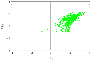
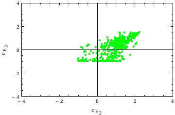
The up and down mass matrices are given in terms of fermion mass matrix of Eq.(II.1). The theory parameters which are varied simultaneously to minimise the $\chi^{2}$ in Eq.(13) include: three $c_{Q_{i}}$, each of $c_{u_{i}}$ and $c_{d_{i}}$ and 18 $\mathcal{O}(1)$ Yukawa parameters. We would expect that the light quarks would be localised close to the UV brane ( $c>1/2$ ) and the heavy quarks close to the IR brane ($c<1/2$). However, for this particular range of $\mathcal{O}(1)$ Yukawa parameters, it is difficult to fit the data for $|c|$ within unity. We thus enlarged the range for the $c$ parameters.

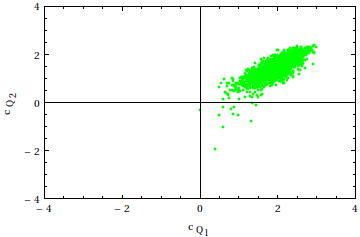
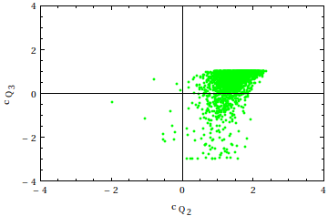
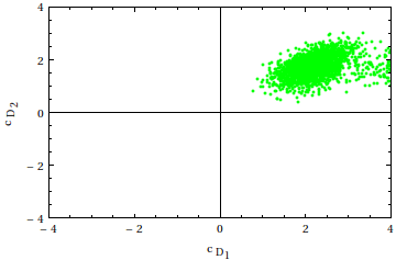
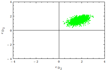
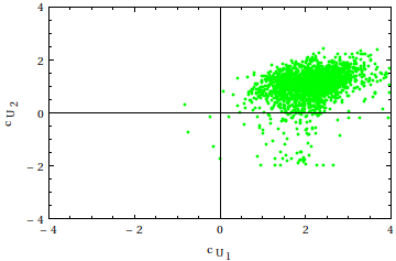
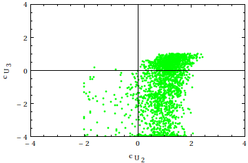
The range chosen for the scan of the $c$ parameters chosen is: $-2<c_{Q_{1},Q_{2}}<4$, $-3<c_{Q_{3}}<1$ for the doublets. $-2<c_{d_{1},d_{2},d_{3}}<3.5$, for the down type singlets and $-2<c_{u_{1},u_{2}}<4$, $-4<c_{u_{3}}<1$ for the up type singlets. We fit the quark masses and the CKM mixing angles at the GUT scale. The top quark is definitely lighter at the GUT scale, but still we see that most of the points that fit the data lie outside of $|c|~{}\leq~{}1$. This is evident from the the negative values of the $c_{Q_{3}}$ and $c_{U_{3}}$ that fit the data.

The regions of $c$ parameter space which satisfy the constraint of $0<\chi^{2}<10$ for the chosen scanning range are shown in Fig.(1) in Appendix A and the ranges are outlined in Table[3]. We see that the first two generation bulk mass parameters are concentrated on the positive $c$ values where as the third generation, the doublet and more so the right handed top is localised close to the GUT scale brane. Comparing these results with that of the normal RS, we find that the masses for the light quark fields can be fit with $c\sim 0.6-0.7$. This can be attributed to the large warping where $0.5<c<1$ is sufficient to reproduce the masses for light quarks Hubershafi .

Table 3: Allowed range of $c$ parameters in the SM case. These parameters satisfy $0<\chi^{2}<10$ for the SM case. The corresponding figure is 1 in Appendix A.

parameter	range	parameter	range	parameter	range
$c_{Q_{1}}$	[0,3.0]	$c_{D_{1}}$	[0.78,4]	$c_{U_{1}}$	[-0.97,3.98]
$c_{Q_{2}}$	[-1.95,2.36]	$c_{D_{2}}$	[0.39,3.02]	$c_{U_{2}}$	[-1.99,2.43]
$c_{Q_{3}}$	[-3,1]	$c_{D_{3}}$	[0.39,2.21]	$c_{U_{3}}$	[-4,1.0]

III.1.2 SM Leptonic Mass fits

Unlike the quark case, the fits in the leptonic sector are far more difficult and more constraining due to the small mass differences and the large mixing in the neutrino sector. As mentioned, we will consider two different cases of neutrino masses while fitting the leptonic data.

(a) LLHH higher dimensional operator
Planck scale lepton number violation is an interesting idea which manifests itself with higher dimensional operator suppressed by the Planck scale. In four dimensions such an operator generates too small neutrino mases. It is typically used as a perturbation over an existing neutrino mass model umashankar . If not, it needs an enhancement of $\mathcal{O}(10^{3}-10^{4})$ to be consistent with the data. In the standard RS framework close to the weak scale with bulk fermions, this higher dimensional operator is still constrained however for different reasons. While the neutrino masses can be fit by placing the doublet fields $L$ close to the UV brane, the charged lepton masses become very tiny unless the singlet fields (E) are placed deep in the IRiyer . This leads to inconsistencies in the theory with large non-perturbative Yukawa couplings. The question arises whether the situation repeats itself when we consider the modified RS setup. This can be checked as follows. The neutrino masses are generated by the higher dimensional operator as given in Eq.(II.1). The corresponding neutrino mass matrix is given by Eq.(5) while the mass matrix for the charged leptons is given by Eq.(II.1).

For simplicity assume $c_{L_{i}}=c_{L}\forall$ i. For $c_{L}<0.5$ the mass matrix in Eq.(5) becomes

$$m_{\nu}=\kappa^{\prime}\frac{v^{2}sin^{2}(\beta)}{2\epsilon\Lambda}(1-2c_{L})$$ (14)

It is clear that $c_{L}\sim-4$ is required to get neutrino masses $\mathcal{O}(0.04)$ eV for a warp factor for $\epsilon\sim 10^{-2}$. As $c_{L}$ increases, beyond 0.5, this formula is no longer valid, the neutrino masses become smaller and hence do not fit the neutrino mass data with $\mathcal{O}(1)$ Yukawa couplings. Thus a mildly negative $c_{L}$ should be able to fit the data without large inconsistencies.

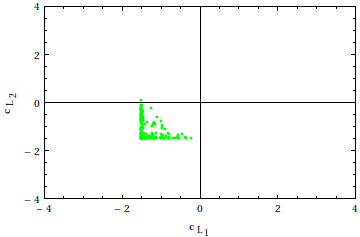
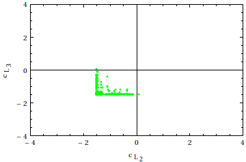
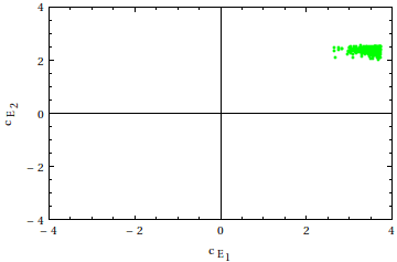
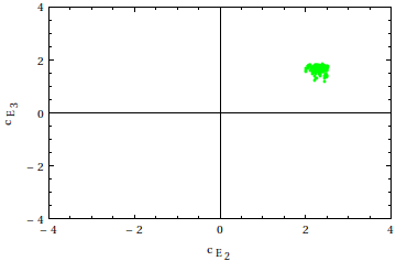
A second enhancement can also come from the $\kappa^{\prime}$, which is the corresponding $\mathcal{O}(1)$ Yukawa. With this in mind, we enhance the range of the scanning of the Yukawa couplings from $0.08$ to $4$ to $0.08$ to $10$. This would help us to accommodate $c_{L}$ values close to $\sim-1$. The final scanning ranges we have chosen are: the doublets ($c_{L_{i}}$) are varied between -1.5 and 0.5, while the charged singlets were scanned between 0 and 4. The region of $c$ values which give a good fit to leptonic masses, i.e, satisfying the constraint $0<\chi^{2}<10$, is presented in Table[4]. The plots for these ranges of $c$ values are presented in Figs.(2) in Appendix A.

Table 4: Ranges for scanned regions of the bulk leptonic parameters for the LLHH in the SM case which satisfy $0<\chi^{2}<10$.

parameter	range	parameter	range
$c_{L_{1}}$	[ -1.5,-1.15]	$c_{E_{1}}$	[2.8,4.0]
$c_{L_{2}}$	[-1.5,-0.97]	$c_{E_{2}}$	[1.8,2.4]
$c_{L_{3}}$	[-1.5,-1.22]	$c_{E_{3}}$	[1.2,1.69]

(b)Dirac type Neutrinos
The case of Dirac neutrinos is interesting possibility though it requires imposition of a global lepton number conservation. The running of the neutrino masses from the weak scale to high scale is different in this case. However with a normal hierarchy of neutrinos and low tan$\beta$ the differences are insignificantxing2 ; xing3 .

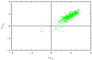
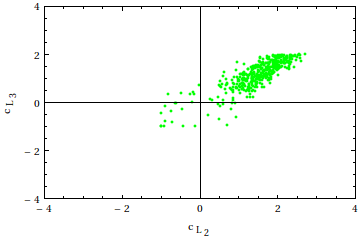
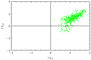
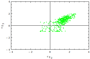
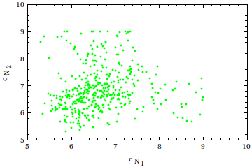
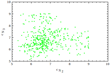
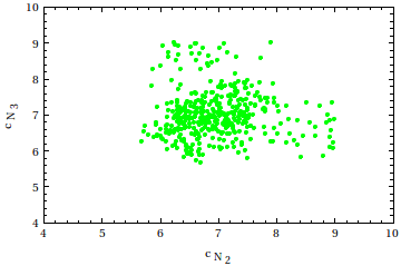
Assuming that there is not much of a difference for normal hierarchy, we choose the following scanning range for the $c$ parameters. The doublets ($c_{L_{i}}$) and charged lepton singlets ($c_{E_{i}}$) are scanned within the range -1 to 4.5, while the neutrino singlets were scanned in the range 3.5 to 9. Such a large value of the bulk mass parameters for the singlets is needed to suppress the corresponding neutrino masses sufficiently. The $\mathcal{O}$(1) Yukawa parameters were varied between 0.08 and 4. Comparing the results of Dirac neutrino mass fits with that of the weak scale RS models,iyer , we find that the $c_{N}$ are roughly a factor $7-8$ larger compared to the $c_{N}$ at the weak scale. This is purely because of the weaker warp factor we are considering in the present case. Increasing the range of the $O(1)$ Yukawa parameters would only make things worse. The ranges for the $c$ values corresponding to SM fits with Dirac neutrinos case are presented Table[5]. The plots for the $c$ parameters are presented case in Fig[3] in Appendix A.

Table 5: Ranges for the scanned regions of the bulk leptonic parameters for the Dirac case which satisfy $0<\chi^{2}<10$ for the SM case.

parameter	range	parameter	range	parameter	range
$c_{L_{1}}$	[ -1,2.9]	$c_{E_{1}}$	[0.39,3.62]	$c_{N_{1}}$	[5.29,8.97]
$c_{L_{2}}$	[-0.99,2.7]	$c_{E_{2}}$	[-1.0,2.63]	$c_{N_{2}}$	[5.31,8.99]
$c_{L_{3}}$	[-0.99,1.98]	$c_{E_{3}}$	[-0.99,1.93]	$c_{N_{3}}$	[5.12,8.97]

III.2 Supersymmetric Case

The analysis for the case with bulk supersymmetry is similar to the SM case. The GUT scale values are derived using the supersymmetric RGE at the two loop instead of the SM ones. For the neutrinos however, one loop RGE were used with experimental inputs at the weak scale. The running of the masses are not dependent on the mixing angles for a low tan$\beta$. Supersymmetry threshold corrections can play an important role while deriving the running masses. Running masses in the supersymmetric framework were obtained using the relevant matching conditions. As is well known, these effects are significant at large tan$\beta$ and the corrections to the neutrino running through $Y_{D}$ and $Y_{E}$ were considered Antusch .

The GUT scale masses and mixings chosen for the scan corresponded to tan$\beta=10$ and are given in Table[6] and [7]. The results of the the scan i.e, the ranges for the $c$ parameters are weakly dependent on tan$\beta$ and can be applied for studying phenomenology for up to tan$\beta\sim 25$.

Table 6: GUT scale Masses with supersymmetry for tan$\beta=10$

Mass	Mass	Mass	Mass squared Differences
(MeV )	(GeV)	MeV	$eV^{2}$
$m_{u}=0.49^{+0.20}_{-0.17}$	$m_{c}=0.236^{+0.037}_{-0.036}$	$m_{e}=0.28^{+0.0000007}_{-0.0000007}$	$\Delta m^{2}_{12}=1.6^{+0.20}_{-0.21}\times 10^{-4}$
$m_{d}=0.70^{+0.31}_{-0.31}$	$m_{b}=0.79^{+0.04}_{-0.04}$	$m_{\mu}=59.9^{+0.000005}_{-0.000005}$	$\Delta m_{23}^{2}=3.2^{+0.13}_{-0.13}\times 10^{-3}$
$m_{s}=13^{+4}_{-0.4}$	$m_{t}=92.2^{+9.6}_{-7.8}$	$m_{\tau}=1021^{+0.1}_{-0.1}$	-

Table 7: Mixing angles for the quarks and leptons at GUT scale with supersymmetry for tan$\beta=10$

mixing angles(CKM)	Mixing angles (PMNS)
$\theta_{12}=0.226^{+0.00087}_{-0.00087}$	$\theta_{12}=0.59^{+0.02}_{-0.015}$
$\theta_{23}=0.0415^{+0.00019}_{-0.00019}$	$\theta_{23}=0.79^{+0.12}_{-0.12}$
$\theta_{13}=0.0035^{+0.001}_{-0.001}$	$\theta_{13}=0.154^{+0.016}_{-0.016}$

III.2.1 Quark Case

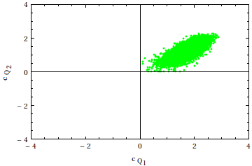
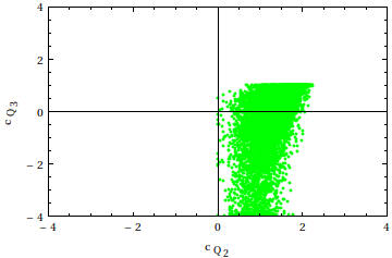
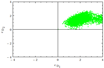
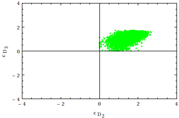
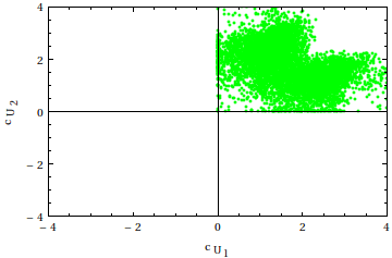
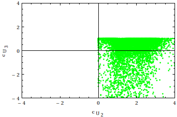
The range chosen for the scan are the same as that for the SM case i.e. $-2<c_{Q_{1},Q_{2}}<4$, $-3<c_{Q_{3}}<1$ for the doublets. $-2<c_{d_{1},d_{2},d_{3}}<3.5$, for the down type singlets and $-2<c_{u_{1},u_{2}}<4$, $-4<c_{u_{3}}<1$ for the up type singlets. The regions of $c$ parameter space which satisfy the constraint of $0<\chi^{2}<10$ for the chosen scanning range are shown in Fig.(4) in Appendix B and the ranges are outlined in Table[8].

Table 8: Ranges for the scanned regions of bulk hadronic parameters which satisfy $0<\chi^{2}<10$ for the supersymmetric case.

parameter	range	parameter	range	parameter	range
$c_{Q_{1}}$	[-0.16,3.12]	$c_{D_{1}}$	[-0.5,4]	$c_{U_{1}}$	[-1.6,4.0]
$c_{Q_{2}}$	[-1.32,2.34]	$c_{D_{2}}$	[-1.9,2.5]	$c_{U_{2}}$	[-2,2.4]
$c_{Q_{3}}$	[-3,1]	$c_{D_{3}}$	[-2,1.7]	$c_{U_{3}}$	[-4,1.0]

III.2.2 Leptonic case

Similar to the SM scenario two cases of neutrino mass generation are considered. The GUT scale input values for the $\chi^{2}$ is given in Table[6] and [7].

(a)LLHH case
The results of the scan of the LLHH case is very similar for both the SM case and the supersymmetric case. The expression for the neutrino mass matrix is given in Eq.(12). For the neutrino sector we allow the $\mathcal{O}$(1) Yukawa coupling to vary between -10 and 10 with a minimum of 0.08 while that for the charged leptons are varied between -4 and 4 with a minimum of 0.08. The doublets were scanned between -1.5 and 0.5 while the charged singlets were scanned between 0 and 4. The ranges for the $c$ parameters for the LLHH case for the chosen scanning range satisfying the constraint $0<\chi^{2}<10$, is presented in Table[9] and the plots for the $c$ values are presented in Figs.(5) in Appendix B.

Table 9: Ranges for scanned regions of the bulk leptonic parameters for the LLHH scenario in the supersymmetric case which satisfy $0<\chi^{2}<10$.

parameter	range	parameter	range
$c_{L_{1}}$	[ -1.5,-0.22]	$c_{E_{1}}$	[2.6,3.7]
$c_{L_{2}}$	[-1.5,0.08]	$c_{E_{2}}$	[2.0,2.57]
$c_{L_{3}}$	[-1.5,0.04]	$c_{E_{3}}$	[1.1,1.8]

(b)Dirac Neutrinos
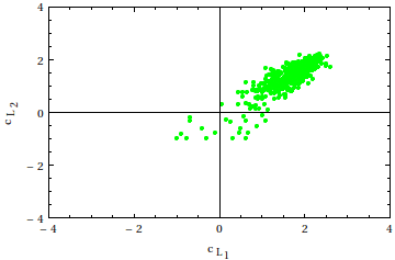
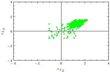
The expression for the mass matrix for the all the leptons is given by Eq.(10) The scanning range for the $c$ values of all the doublets and charged lepton singlets was in the range -1 to 4.5, while the neutrino singlets were scanned in the range 3.5 to 9. The magnitude of $\mathcal{O}$(1) Yukawa parameters were varied between 0.08 and 4. The regions of the $c$ parameters satisfying the constraint $0<\chi^{2}<10$ for the scanned ranges are presented in Table[10]. The ranges are presented in Fig.(6) in Appendix B.

Table 10: Ranges for the scanned regions of the bulk leptonic parameters for the Dirac case with supersymmetry which satisfy $0<\chi^{2}<10$ for the supersymmetric case.

parameter	range	parameter	range	parameter	range
$c_{L_{1}}$	[ -1,2.6]	$c_{E_{1}}$	[-0.86,3.46]	$c_{N_{1}}$	[5.68,8.9]
$c_{L_{2}}$	[-0.99,2.21]	$c_{E_{2}}$	[-1,2.24]	$c_{N_{2}}$	[5.67,8.99]
$c_{L_{3}}$	[-1,1.54]	$c_{E_{3}}$	[-1,1.49]	$c_{N_{3}}$	[5.64,8.99]

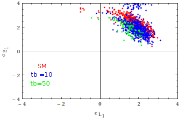
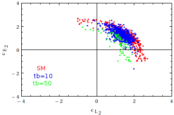
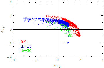
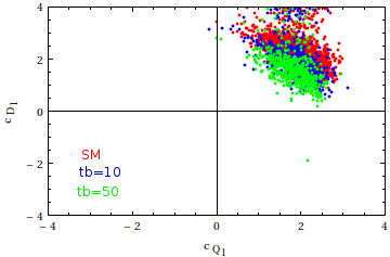
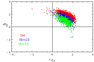
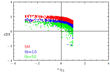
To summarize, on comparing the SM and the SUSY fits, we find that within a given generation, the fields have a tendency to be localized slightly towards the IR for the SUSY case than for the SM case. This effect is more pronounced in the down sector and increases with tan$\beta$. A comparison between the fits for the SM case and the SUSY case for $tan\beta=10$ and $50$ are presented in Figs.[7] in Appendix C. The underlying features of the fit in which the first two generations including the neutrinos are elementary from the ADS/CFT point of view while the third generation fermions $(t_{L},t_{R})$ having a tendency to be partially composite or composite, is maintained for both the SM and the SUSY case. From the choice of the $c$ parameters, we find that the LLHH case admits a better fit to the neutrino data than the Dirac case. This is contrary to the observations made in iyer in normal RS where the $c$ parameters for all the leptons were close to unity. It thus offered a more viable alternative than the LLHH case. In order to compensate for the weak warp factor in the Dirac case the right handed neutrinos had bulk masses $c_{N}\sim 7$. This weak warping however, works in favour of the LLHH case where for $c<0.5$ the effective 4D suppression scale is of the $\mathcal{O}$($M_{GUT}$) resulting in fits with $c$ parameters closer to unity.

IV SUSY Spectrum and Flavour Phenomenology

There are several ways to break supersymmetry within this RS set up at the GUT scale (see for example discussion in choi1 ; choi2 ; Dudas ; Brummer ; nomura . In the present work, we will consider only one particular set up which manifestly demonstrates the flavour structure of the fermions within the soft terms. More detailed analysis of supersymmetric spectrum will be addressed in iyer2 . We will assume in the following that supersymmetric breaking happens on the IR brane, or the GUT brane. Unlike the work of Hallnomura and Brummer we will not arrange the SM fields in any particular GUT representation. As has been discussed in these works, a GUT structure can be arranged with possible solutions for proton decay and doublet triplet splitting. Instead we parameterize SUSY breaking in terms of a single four dimensional spurion chiral superfield, $X=\theta^{2}F$, which is localized on the GUT brane. However, for soft masses generated at the Planck brane as in Dudas , one may then impose the GS anomaly cancellation conditions on bulk masses to ensure unification of couplings at the Planck scale. We do not impose any such conditions as the soft masses are generated at the GUT scale.

In the limit, the higher KK modes are decoupled from the GUT scale physics Marti , the Kähler potential relevant for the scalar mass terms is given by

$$\mathcal{K}^{(4)}=\int dy\delta(y-\pi R)e^{-2k\pi R}k^{-2}X^{\dagger}X\left(\beta_{q,ij}Q^{\dagger}_{i}Q_{j}+\beta_{u,ij}U^{\dagger}_{i}U_{j}+\beta_{d,ij}D^{\dagger}_{i}D_{j}+\gamma_{u,d}H_{u,d}^{\dagger}H_{u,d}+\ldots\right)$$ (15)

where $\beta$ have dimensional carrying negative mass dimensions of -1 ( as the matter fields are five dimensional). $\gamma_{u,d}$ are $\mathcal{O}(1)$ parameters.

The sfermion mass matrix is generated when the $X$ fields get a vacuum expectation value $m_{\tilde{f}}^{2}\sim k^{-2}<X>^{\dagger}<X>Q^{\dagger}Q$. The mass matrix will however not be diagonal in flavour space. In the canonical basis, (15), the mass matrices take the form

$$(m_{\tilde{f}}^{2})_{ij}=m_{3/2}^{2}~{}\hat{\beta}_{ij}~{}e^{(1-c_{i}-c_{j})kR\pi}\xi(c_{i})\xi(c_{j})$$ (16)

where $\hat{\beta}_{ij}=2k\beta_{ij}$ are dimensionless $\mathcal{O}(1)$ parameters. $\xi(c_{i})$ are defined in Eq.(II.1). And the gravitino mass is defined as

$$m_{3/2}^{2}={<F>^{2}\over k^{2}}={<F>^{2}\over M_{Pl}^{2}}$$ (17)

The Higgs fields are localised on the GUT brane, their masses are given by $m^{2}_{H_{u},H_{d}}=\gamma_{u,d}~{}m_{3/2}^{2}$.

The A-terms are generated from the higher dimensional operators in the super potential of the type :

$$W^{(4)}=\int dy\delta(y-\pi R)e^{-3ky}k^{-1}X\left(\tilde{A}^{u}_{ij}H_{u}Q_{i}u_{j}+\tilde{A}^{d}_{ij}H_{d}Q_{i}d_{j}+\tilde{A}^{e}_{ij}H_{d}L_{i}E_{j}+\ldots\right)$$ (18)

where the $\tilde{A}$ are dimensionful parameters having mass dimension -1. Substituting for the vev of the $X$, we have for the four dimensional trilinear couplings at the GUT scale:

$$A^{u,d}_{ij}=m_{3/2}A^{\prime}_{ij}e^{(1-c_{i}-c^{\prime}_{j})kR\pi}\xi(c_{i})\xi(c^{\prime}_{j})$$ (19)

where we defined the dimensionless $\mathcal{O}(1)$ parameters as $A^{\prime}=2k\tilde{A}$. The structure of the A terms and the corresponding fermion mass matrix are similar and they differ only by the choice of the $\mathcal{O}$(1) parameters. Choosing $A^{\prime}=2kY^{\prime}$, makes the down sector A terms diagonal in the mass basis of the fermions at the GUT scale. Henceforth, we shall work in this basis, with the $\mathcal{O}$(1) parameters of the A terms proportional to the $\mathcal{O}$(1) Yukawa parameters.

The masses for the gauginos are obtained from the following operator in the lagrangian

$$\mathcal{L}=\int d^{2}\theta k^{-1}X\mathcal{W}_{A\alpha}\mathcal{W}^{\alpha}_{A}$$ (20)

At $M_{GUT}$ their masses will be be $m_{1/2}=fm_{3/2}$ where $f$ is a $\mathcal{O}(1)$ parameter. $m_{1/2}$ will be treated as an independent parameter. They are independent of the position of localization of X. as the profile for the gauginos is flat corresponding to a bulk mass parameter of 0.5 Marti ; Gherghetta1 .

While the above equations set the boundary conditions at the high scale, the weak scale spectrum is determined by the RGE evolution. In the present case, the spectrum at the high scale is completely non-universal as determined by the profiles of the zero modes of the matter chiral superfields. The structure of soft terms discussed here is similar to the ideas of flavourful supersymmetry discussed by Nomura1 ; Nomura2 and more recently by Ramond . In the following we will present two example points one for the LHLH higher dimensional operator case and another for the Dirac case.

To begin with, in both the examples, we consider that all the $\mathcal{O}(1)$ parameters appearing in the definitions of the soft parameters are proportional to the unit matrix. We will explicitly mention any deviations as required by the phenomenology when presenting numerical examples. This would mean that the matrices, $A^{\prime},\hat{\beta}$ in Eqs. (16, 19) are proportional to unit matrix and the parameters $\gamma_{u},\gamma_{d}$ in Eq.(15) are equal to one. However, as we will see below, they play an important role in low energy phenomenology and one might frequently require to vary them within the $\mathcal{O}(1)$ range, to satisfy phenomenological constraints. While studying the flavour phenomenology, we make sure that the soft terms are present in the super-CKM basis. The low-energy spectrum has been computed numerically using the spectrum generator SUSEFLAV suseflav .

IV.0.1 LHLH operator case

In this case we consider the following point, (21), in the $c$ parameter space. It has a $\chi^{2}$ of $5.5$ for the hadronic sector and $0.7341$ for the leptonic sector. As expected it has a mostly composite right handed top quark. In addition, the leptonic doublets are also significantly composite in this case.

$$c_{Q_{1}}=2.740\hskip 14.22636ptc_{D_{1}}=0.722\hskip 14.22636ptc_{U_{1}}=0.4024\hskip 14.22636ptc_{L_{1}}=-1.497\hskip 14.22636ptc_{E_{1}}=3.634$$

$$c_{Q_{2}}=1.920\hskip 14.22636ptc_{D_{2}}=0.729\hskip 14.22636ptc_{U_{2}}=0.0652\hskip 14.22636ptc_{L_{2}}=-0.224\hskip 14.22636ptc_{E_{2}}=2.290$$

$$c_{Q_{3}}=0.960\hskip 14.22636ptc_{D_{3}}=0.801\hskip 14.22636ptc_{U_{3}}=-3.5615\hskip 14.22636ptc_{L_{3}}=-1.0738\hskip 14.22636ptc_{E_{3}}=1.769$$ (21)

The choice of $\mathcal{O}$(1) parameters in the soft sector plays a role in determining the nature of the low energy spectrum. For a given set of $c$ parameters, a naive choice of one for all the $\mathcal{O}$(1) parameters in the soft sector may or may not lead to an acceptable spectrum at $M_{susy}$. For the LLHH case corresponding to the choice in Eq.(21) the $\mathcal{O}$(1) parameters for all the soft masses are taken to be 1. The $\mathcal{O}$(1) parameters for the A terms are chosen to be $\hat{A}^{u}=1.02Y^{{}^{\prime}u}$ while $\hat{A}^{u}=Y^{{}^{\prime}d}$ and $\hat{A}^{e}=0.6Y^{{}^{\prime}e}$. Corresponding to these choices of the $\mathcal{O}$(1) parameters and the $c$ values in Eq.(21), the soft breaking terms at the GUT scale in $GeV$ are given as:

$$m_{Q}=\begin{bmatrix}0.001&-0.03&-0.27\\ -0.03&0.85&7.6\\ -0.27&7.6&68.7\end{bmatrix};m_{U}=\begin{bmatrix}11.5&-63.5&156.1\\ -63.5&349.6&-859.1\\ 156.1&-859.1&2110.8\end{bmatrix};m_{D}=\begin{bmatrix}105.03&-90.4&155.2\\ -90.4&77.8&-133.6\\ 155.2&-133.6&229.5\end{bmatrix}$$

$$A_{U}=\begin{bmatrix}-0.002&-0.09&-0.84\\ -0.0002&1.09&-6.3\\ -10^{-6}&0.01&439.4\end{bmatrix};A_{D}=\begin{bmatrix}0.03&0&0\\ 0&-0.40&0\\ 0&0&-40.6\end{bmatrix};m_{L}=\begin{bmatrix}7.7&8.8&-147.5\\ 8.8&9.9&-167.0\\ -147.5&-167.0&2798.4\end{bmatrix}$$

$$m_{E}=\begin{bmatrix}0.001&-0.017&0.05\\ -0.017&0.26&-0.89\\ 0.05&-0.89&3.04\end{bmatrix};A_{E}=\begin{bmatrix}0.008&0&0\\ 0&1.81&0\\ 0&0&-31.3\end{bmatrix}$$ (22)

A couple of interesting features of the above spectrum are (i) at least one of the soft masses is tachyonic (ii) significant amount of flavour violation present at the high scale. However at the weak scale, things are significantly different. This is because the RG running is quite different for the diagonal terms compared to the off-diagonal ones. In fact, the off-diagonal entries barely run, where as the corrections to the diagonal ones are quite significant. As an illustration, consider the slepton mass matrix at the weak scale. The analytic output at the weak scale for the diagonal terms can be approximated as

$$\tilde{M}^{2}_{L_{1,2}}\simeq m_{L_{1,2}}^{2}+0.5M_{1/2}^{2}$$ (23)

$$\tilde{M}^{2}_{L_{3}}\simeq m_{L_{3}}^{2}+0.5M_{1/2}^{2}$$

$$\tilde{M}^{2}_{E_{1,2}}\simeq m_{E_{1,2}}^{2}+0.15M_{1/2}^{2}$$

$$\tilde{M}^{2}_{E_{3}}\simeq m_{E_{3}}^{2}+0.15M_{1/2}^{2}$$

which receive gauge contributions while the off diagonal elements do not. The A terms are not large enough to make the off diagonal elements of the soft mass matrices comparable with the diagonal terms. An example for the sleptons for the case under consideration is given as

$$m_{L}^{2}(m_{susy}) = \begin{bmatrix}2.2\times 10^{5}&77.0&-2.1\times 10^{4}\\ 77.0&2.2\times 10^{5}&-2.7\times 10^{4}\\ -2.1\times 10^{4}&-2.7\times 10^{4}&7.7\times 10^{6}\end{bmatrix}\text{GeV}^{2}$$

$$m_{E}^{2}(m_{susy}) = \begin{bmatrix}1.1\times 10^{6}&3.4\times 10^{-4}&2.2\times 10^{-1}\\ 3.4\times 10^{-4}&1.1\times 10^{6}&5.9\times 10^{1}\\ 2.2\times 10^{-1}&5.9\times 10^{1}&5.4\times 10^{5}\end{bmatrix}\text{GeV}^{2}$$ (24)

We see that the off-diagonal entry has barely enhanced where as the diagonal entries have been significantly modified. Constraints from flavour violation would restrict the mass scales of $m_{3/2}$ and $M_{1/2}$. The most stringent constraints are from the transitions between the first two generations ie from $K^{0}\to\bar{K}^{0}$ and $\mu\to e+\gamma$. The expressions for the $K_{L}-K_{S}$ mass difference and the branching fractions for $\mu\to e+\gamma$ can be found in Gabbiani ; Gabbiani1 . We impose the flavour constraints from all the existing data on the $\delta$ parameters.

Bounds from the flavour violating processes are obtained using the mass insertion approximation Gabbiani and the results of vempati defined in the Super-CKM basis. The flavour violating indices are defined as $\delta_{ij}(i\neq j)={(U^{\dagger}M^{2}_{soft}U)_{ij}\over m_{susy}}(i\neq j)$ are evaluated in the basis in which the down sector is diagonal, with U being the rotation matrix which rotates the corresponding fermion mass matrix. The $\delta$ are evaluated at the weak scale and we scale the bounds of vempati to the present mass scales. In Table[12] we present the low energy spectrum corresponding to the sample point in Eq.(21). The low energy $\delta^{\prime}s$ are presented in Table 13.

Table 11: Experimental upper bounds on the $\delta^{down}$ obtained for $\tilde{m}_{q}=2.1$ TeV and $\tilde{m}_{l}=0.7$ TeV

(i,j)	$|\delta^{Q}_{LL}|$	$|\delta^{L}_{LL}|$	$|\delta^{D}_{LR}|$	$|\delta^{E}_{LR}|$	$|\delta^{D}_{RL}|$	$|\delta^{E}_{RL}|$	$|\delta^{D}_{RR}|$	$|\delta^{E}_{RR}|$
12	0.053	$0.0002$	$0.0003$	$3.8\times 10^{-6}$	$0.0003$	$3.8\times 10^{-6}$	0.03	0.03
13	$0.34$	0.14	$0.06$	$0.03$	0.06	$0.03$	0.26	-
23	0.61	$0.16$	$0.01$	0.04	$0.02$	0.04	0.84	-

Table 12: Soft spectrum for LLHH case: $m_{susy}=1.06$ TeV, $m_{\tilde{g}}=2.64$ TeV, $\mu=3.43$TeV, $tan\beta=25$

Parameter	Mass(TeV)	Parameter	Mass(TeV)	Parameter	Mass(TeV)	Parameter	Mass(Tev)	Parameter	Mass(TeV)
$\tilde{t}_{1}$	0.47	$\tilde{b}_{1}$	1.01	$\tilde{\tau}_{1}$	0.726	$\tilde{\nu}_{\tau}$	2.78	$N_{1}$	0.465
$\tilde{t}_{2}$	1.05	$\tilde{b}_{2}$	2.14	$\tilde{\tau}_{2}$	2.79	$\tilde{\nu}_{\mu}$	0.483	$N_{2}$	0.929
$\tilde{c}_{R}$	2.24	$\tilde{s}_{R}$	2.40	$\tilde{\mu}_{R}$	0.478	$\tilde{\nu}_{e}$	0.469	$N_{3}$	3.38
$\tilde{c}_{L}$	2.48	$\tilde{s}_{L}$	2.48	$\tilde{\mu}_{L}$	1.05	-	-	$N_{4}$	3.39
$\tilde{u}_{R}$	2.24	$\tilde{d}_{R}$	2.40	$\tilde{e}_{R}$	0.476	-	-	$C_{1}$	0.895
$\tilde{u}_{L}$	2.48	$\tilde{d}_{L}$	2.48	$\tilde{e}_{L}$	1.05	-	-	$C_{2}$	3.43
$m_{A^{0}}$	3.23	$m_{H}^{\pm}$	3.23	$m_{h}$	0.12186	$m_{H}$	3.06	-	-

Table 13: Low energy $\delta^{\prime}s$ for quarks and leptons corresponding to the points in Eq.(21) for the LLHH case evaluated for $\tilde{m}_{q}=2.1$TeV and $\tilde{m}_{l}=0.7$ TeV

(i,j)	$|\delta^{Q}_{LL}|$	$|\delta^{L}_{LL}|$	$|\delta^{D}_{LR}|$	$|\delta^{U}_{LR}|$	$|\delta^{D}_{RL}|$	$|\delta^{U}_{RL}|$	$|\delta^{D}_{RR}|$	$|\delta^{E}_{RR}|$	$|\delta^{U}_{RR}|$
12	0.0003	$0.0001$	$10^{-10}$	$10^{-8}$	$10^{-8}$	$10^{-5}$	$0.001$	$10^{-10}$	0.001
13	$0.01$	0.04	$10^{-8}$	$10^{-8}$	$10^{-6}$	$0.002$	$0.005$	$10^{-7}$	0.01
23	0.05	$0.05$	$10^{-6}$	$10^{-5}$	$10^{-5}$	$0.01$	$0.003$	0.0001	0.07

IV.0.2 Dirac Case

For the case where neutrinos are of Dirac type the $c$ parameters in Eq.(25) with $\chi^{2}$ of $0.3211$ for the hadronic sector and $0.1481$ for the leptonic sector were chosen. The $c$ values for the doublets in this case indicate they are predominantly elementary from the CFT point of view especially for the first two generations. The third generation however may be partially composite as in this case.

$$c_{Q_{1}}=1.895\hskip 14.22636ptc_{D_{1}}=1.898\hskip 14.22636ptc_{U_{1}}=1.738\hskip 14.22636ptc_{L_{1}}=1.293\hskip 14.22636ptc_{E_{1}}=2.480\hskip 14.22636ptc_{N_{1}}=6.783$$

$$c_{Q_{2}}=1.467\hskip 14.22636ptc_{D_{2}}=1.271\hskip 14.22636ptc_{U_{2}}=1.124\hskip 14.22636ptc_{L_{2}}=1.311\hskip 14.22636ptc_{E_{2}}=1.406\hskip 14.22636ptc_{N_{2}}=7.346$$

$$c_{Q_{3}}=-0.137\hskip 14.22636ptc_{D_{3}}=1.394\hskip 14.22636ptc_{U_{3}}=-0.356\hskip 14.22636ptc_{L_{3}}=0.260\hskip 14.22636ptc_{E_{3}}=0.237\hskip 14.22636ptc_{N_{1}}=7.332$$ (25)

The generic feature of soft mass matrices, discussed in the LLHH case, of the spectrum being tachyonic at the high scale and the diagonal terms evolving more than the off diagonal elements apply to this case as well. Corresponding to the c values in Eq.(25), the soft masses at the GUT scale have been evaluated for $m^{GUT}_{3/2}=800$ GeV while choosing $M_{1/2}=1200$ GeV for the three gauginos. The $\mathcal{O}(1)$ parameters corresponding to $(m_{Q})_{33}$ and $(m_{U})_{33}$ were chosen to be 4 while for the others they are set to be 1. $A^{{}^{\prime}u}_{ij}=1.15Y^{{}^{\prime}u}\forall i,j$, for all the A terms of the up sector while for the down sector and the leptons they were set equal to the corresponding $\mathcal{O}$(1) Yukawa couplings. The high scale soft breaking matrices in $GeV$ are given in Eq.(26). In Table[14] we present the low energy spectrum corresponding to the sample point in Eq.(25). The low energy $\delta^{\prime}s$ are presented in Table 15.

$$m_{Q}=\begin{bmatrix}0.60&1.2&30.0\\ 1.2&8.7&-19.4\\ 30.0&-19.4&2560.6\end{bmatrix};m_{U}=\begin{bmatrix}0.7&-3.8&17.1\\ -3.8&32.1&70.3\\ 17.1&70.3&2971.6\end{bmatrix};m_{D}=\begin{bmatrix}0.10&-0.85&-1.7\\ -0.85&7.1&14.6\\ -1.7&14.6&29.8\end{bmatrix}$$

$$A_{U}=\begin{bmatrix}10^{-3}&-0.42&-5.8\\ 10^{-3}&1.18&0.20\\ 10^{-5}&-0.005&488.8\end{bmatrix};A_{D}=\begin{bmatrix}0.03&0&0\\ 0&0.57&0\\ 0&0&-40.6\end{bmatrix};m_{L}=\begin{bmatrix}8.7&0.9&62.5\\ 0.9&0.1&7.0\\ 62.5&7.0&446.3\par\end{bmatrix}$$

$$m_{E}=\begin{bmatrix}0.2&-0.4&10.5\\ -0.4&0.7&-17.9\\ 1.0&-17.29&442.7\end{bmatrix};A_{E}=\begin{bmatrix}-0.01&0&0\\ 0&-3.01&0\\ 0&0&52.1\end{bmatrix}$$ (26)

Table 14: Soft spectrum for Dirac case: $m_{susy}=1.05$ TeV, $m_{\tilde{g}}=2.65$ TeV, $\mu=4.32$TeV, $tan\beta=25$

Parameter	Mass(TeV)	Parameter	Mass(TeV)	Parameter	Mass(TeV)	Parameter	Mass(Tev)	Parameter	Mass(TeV)
$\tilde{t}_{1}$	0.702	$\tilde{b}_{1}$	2.06	$\tilde{\tau}_{1}$	0.480	$\tilde{\nu}_{\tau}$	0.570	$N_{1}$	0.465
$\tilde{t}_{2}$	2.31	$\tilde{b}_{2}$	2.32	$\tilde{\tau}_{2}$	0.802	$\tilde{\nu}_{\mu}$	0.624	$N_{2}$	0.928
$\tilde{c}_{R}$	2.25	$\tilde{s}_{R}$	2.36	$\tilde{\mu}_{R}$	0.608	$\tilde{\nu}_{e}$	0.625	$N_{3}$	4.26
$\tilde{c}_{L}$	2.45	$\tilde{s}_{L}$	2.45	$\tilde{\mu}_{L}$	0.902	-	-	$N_{4}$	4.26
$\tilde{u}_{R}$	2.25	$\tilde{d}_{R}$	2.36	$\tilde{e}_{R}$	0.610	-	-	$C_{1}$	0.894
$\tilde{u}_{L}$	2.45	$\tilde{d}_{L}$	2.45	$\tilde{e}_{L}$	0.903	-	-	$C_{2}$	4.32
$m_{A^{0}}$	4.18	$m_{H}^{\pm}$	4.18	$m_{h}$	0.1235	$m_{H}$	3.96	-	-

Table 15: Low energy $\delta^{\prime}s$ for the Dirac Case corresponding to the point in Eq.(25) for Dirac case evaluated for $\tilde{m}_{q}=2.1$TeV and $\tilde{m}_{l}=0.7$ TeV

(ij)	$|\delta^{Q}_{LL}|$	$|\delta^{L}_{LL}|$	$|\delta^{D}_{LR}|$	$|\delta^{U}_{LR}|$	$|\delta^{D}_{RL}|$	$|\delta^{U}_{RL}|$	$|\delta^{D}_{RR}|$	$|\delta^{E}_{RR}|$	$|\delta^{U}_{RR}|$
12	0.0003	$10^{-6}$	$10^{-10}$	$10^{-8}$	$10^{-8}$	$10^{-5}$	$10^{-7}$	$10^{-7}$	0.00005
13	$0.01$	0.007	$10^{-8}$	$10^{-8}$	$10^{-5}$	$0.002$	$10^{-6}$	$10^{-4}$	0.06
23	0.06	$10^{-4}$	$10^{-6}$	$10^{-5}$	$10^{-5}$	$0.01$	$10^{-4}$	0.0006	0.001

V Outlook

The Randall-Sundrum framework is typically considered to be the geometric avatar of the Froggatt-Nielsen models. In the present work, we have considered a warped extra dimension close to the GUT scale. We fit the quark masses and the CKM mixing angles and determined the range of the $c$ parameters which give a reasonable $\chi^{2}$ fit. The $\mathcal{O}(1)$ parameters associated with the Yukawa couplings have also been varied accordingly. Though the top quark Yukawa is smaller at the high scale compared to the weak scale, it is still large enough that one requires a large negative bulk mass parameter for the right handed top quark. For the leptons, we considered two particular models for neutrino masses (a) with Planck scale lepton number violating operator and (b) Dirac neutrino masses.

The results show that there is a significant difference in the RS models at the weak scale and the RS models at the GUT scale especially if one focuses on the neutrino sector. In the weak scale models, the Planck scale lepton number violating higher dimensional operator was very hard to accommodate with perturbative Yukawa couplings and thus was highly disfavoured. The Dirac and the Majorana cases were favoured though they were strongly constrained by the data from flavour violating rare decays. The situation is sort of reversed in the GUT scale RS models, though not exactly. The higher dimensional Planck scale operator fits the data very well, where as the Dirac case requires larger $c$ values, some times with bulk mass parameters almost an order of magnitude larger than the cut-off scale. In the hadronic sector, the situation is not so dramatic. The top quark Yukawa though reduces at the GUT scale compared to the weak scale, still requires that the right handed top to be located close to the IR, making it a composite as in the weak scale models.

The supersymmetric version of the same set up is far more interesting as it can have possible observable signatures at the weak scale. The main difference in fitting of the fermion masses is due to the presence of the additional parameter $\tan\beta$ in the supersymmetric case. The difference in the $c$ values is not very significant for low values of $\tan\beta$. At large $\tan\beta$, for a given generation, the zero modes are localized more towards the IR brane as compared to the SM case. This effect is more pronounced in the down sector as shown in Figures[7]. We parameterise SUSY breaking by a single spurion field localised on the IR brane. The resultant soft masses depend on the profiles of the zero modes of the chiral superfields and contain flavour violation. At the weak scale the constraints from first two generation flavour transitions rule out light spectrum. Another significant constraint comes the light Higgs mass at 125 GeV. The trilinear couplings have the same form as the Yukawa couplings in this model as long as the $\mathcal{O}$(1) parameters associated with both the parameters are taken to be proportional to each other. If all the $\mathcal{O}(1)$ parameters at high scale are take to be exactly unity, the weak scale values of $A_{t}$ are small to generate a 125 GeV light Higgs, for stops of masses $\sim 1.5-2$ TeV. However, with a minor variation of the $\mathcal{O}(1)$ parameters for $A_{t}$ at the high scale, 125 GeV Higgs is easily possible. More variations of supersymmetric breaking and the corresponding spectra will be discussed later iyer2 .

Acknowledgments

We thank Emilian Dudas for discussions and collaboration in the initial stages of this work. We also thank him for a clarification about a point. AI would like to thank CPhT Ecole Polytechnique for hospitality during his stay and Gero Von Gersdorff for useful discussions. We also thank Debtosh Chowdhury for useful inputs. We thank S. Uma Sankar for a reference and communications. SKV acknowledges support from DST Ramanujam fellowship SR/S2/RJN-25/2008 of Govt. of India.

Appendix A Plots for ranges of c parameters for quarks and leptons for SM fits at the GUT scale

A.1 Range of c parameters for the quarks

Figure 1: The points in the above figures correspond to a $\chi^{2}$ between 1 and 10 for the SM fits at the GUT scale. The plot represents the parameter space for the bulk masses of the quarks.

A.2 Range of c parameters for the for leptons for the LLHH scenario

Figure 2: The points in the above figures correspond to a $\chi^{2}$ between 1 and 10. The plot represents the parameter space for the bulk masses of the leptons corresponding to the LLHH case.

A.3 Range of c parameters for the leptons.

Figure 3: The points in the above figures correspond to a $\chi^{2}$ between 1 and 10 for the SM fits at the GUT scale. The plot represents the parameter space for the bulk masses of the leptons corresponding to the Dirac type neutrinos.

Appendix B Plots for ranges of c parameters for quarks and leptons for the supersymmetric case

B.1 Range of c parameters for the quarks

Figure 4: The points in the above figures correspond to a $\chi^{2}$ between 1 and 10. The plot represents the parameter space for the bulk masses of the quarks.

B.2 Range of c parameters for the for leptons for the LLHH scenario

Figure 5: The points in the above figures correspond to a $\chi^{2}$ between 1 and 10. The plot represents the parameter space for the bulk masses of the leptons corresponding to the LLHH case.

B.3 Range of c parameters for the for leptons for the case of Dirac neutrinos.

Figure 6: The points in the above figures correspond to a $\chi^{2}$ between 1 and 10. The plot represents the parameter space for the bulk masses of the leptons corresponding to the Dirac type neutrinos.

Appendix C Comparative plot between SM and supersymmetric fits for fermions

Figure 7: The plots correspond to comparison between SM and supersymmetric fits for down sector fermions. Red corresponds to SM, while Blue and Green corresponds to supersymmetric case for tan$\beta=10$ and tan$\beta=50$ respectively

References

- (1) C. Froggatt and H. B. Nielsen, “Hierarchy of Quark Masses, Cabibbo Angles and CP Violation,” Nucl.Phys., vol. B147, p. 277, 1979.
- (2) K. Babu, “TASI Lectures on Flavor Physics,” pp. 49–123, 2009.
- (3) E. Dudas, S. Pokorski, and C. A. Savoy, “Yukawa matrices from a spontaneously broken Abelian symmetry,” Phys.Lett., vol. B356, pp. 45–55, 1995.
- (4) J. Espinosa and A. Ibarra, “Flavor symmetries and Kahler operators,” JHEP, vol. 0408, p. 010, 2004.
- (5) S. F. King, I. N. Peddie, G. G. Ross, L. Velasco-Sevilla, and O. Vives, “Kahler corrections and softly broken family symmetries,” JHEP, vol. 0507, p. 049, 2005.
- (6) L. E. Ibanez and G. G. Ross, “Fermion masses and mixing angles from gauge symmetries,” Phys.Lett., vol. B332, pp. 100–110, 1994.
- (7) P. Binetruy and P. Ramond, “Yukawa textures and anomalies,” Phys.Lett., vol. B350, pp. 49–57, 1995.
- (8) P. Binetruy, S. Lavignac, and P. Ramond, “Yukawa textures with an anomalous horizontal Abelian symmetry,” Nucl.Phys., vol. B477, pp. 353–377, 1996.
- (9) E. J. Chun and A. Lukas, “Quark and lepton mass matrices from horizontal U(1) symmetry,” Phys.Lett., vol. B387, pp. 99–106, 1996.
- (10) H. K. Dreiner, H. Murayama, and M. Thormeier, “Anomalous flavor U(1)(X) for everything,” Nucl.Phys., vol. B729, pp. 278–316, 2005.
- (11) H. K. Dreiner, C. Luhn, and M. Thormeier, “What is the discrete gauge symmetry of the MSSM?,” Phys.Rev., vol. D73, p. 075007, 2006.
- (12) S. F. King, I. N. Peddie, G. G. Ross, L. Velasco-Sevilla, and O. Vives, “Kahler corrections and softly broken family symmetries,” JHEP, vol. 0507, p. 049, 2005.
- (13) J. R. Ellis, S. Lola, and G. G. Ross, “Hierarchies of R violating interactions from family symmetries,” Nucl.Phys., vol. B526, pp. 115–135, 1998.
- (14) A. S. Joshipura, R. D. Vaidya, and S. K. Vempati, “U(1) symmetry and R-parity violation,” Phys.Rev., vol. D62, p. 093020, 2000.
- (15) P. H. Chankowski, K. Kowalska, S. Lavignac, and S. Pokorski, “Update on fermion mass models with an anomalous horizontal U(1) symmetry,” Phys.Rev., vol. D71, p. 055004, 2005.
- (16) Z. Lalak, S. Pokorski, and G. G. Ross, “Beyond MFV in family symmetry theories of fermion masses,” JHEP, vol. 1008, p. 129, 2010.
- (17) I. de Medeiros Varzielas and G. Ross, “Family symmetries and the SUSY flavour problem,”
- (18) M. Leurer, Y. Nir, and N. Seiberg, “Mass matrix models: The Sequel,” Nucl.Phys., vol. B420, pp. 468–504, 1994.
- (19) M. Leurer, Y. Nir, and N. Seiberg, “Mass matrix models,” Nucl.Phys., vol. B398, pp. 319–342, 1993.
- (20) N. Arkani-Hamed and M. Schmaltz, “Hierarchies without symmetries from extra dimensions,” Phys.Rev., vol. D61, p. 033005, 2000.
- (21) L. Randall and R. Sundrum, “A Large mass hierarchy from a small extra dimension,” Phys.Rev.Lett., vol. 83, pp. 3370–3373, 1999.
- (22) G. Cacciapaglia, C. Csaki, J. Galloway, G. Marandella, J. Terning, et al., “A GIM Mechanism from Extra Dimensions,” JHEP, vol. 0804, p. 006, 2008.
- (23) S. J. Huber and Q. Shafi, “Fermion masses, mixings and proton decay in a Randall-Sundrum model,” Phys.Lett., vol. B498, pp. 256–262, 2001.
- (24) K. Agashe, G. Perez, and A. Soni, “Flavor structure of warped extra dimension models,” Phys.Rev., vol. D71, p. 016002, 2005.
- (25) C. Delaunay, O. Gedalia, S. J. Lee, G. Perez, and E. Ponton, “Ultra Visible Warped Model from Flavor Triviality and Improved Naturalness,” Phys.Rev., vol. D83, p. 115003, 2011.
- (26) K. Agashe, A. E. Blechman, and F. Petriello, “Probing the Randall-Sundrum geometric origin of flavor with lepton flavor violation,” Phys.Rev., vol. D74, p. 053011, 2006.
- (27) K. Agashe, T. Okui, and R. Sundrum, “A Common Origin for Neutrino Anarchy and Charged Hierarchies,” Phys.Rev.Lett., vol. 102, p. 101801, 2009.
- (28) S. Casagrande, F. Goertz, U. Haisch, M. Neubert, and T. Pfoh, “Flavor Physics in the Randall-Sundrum Model: I. Theoretical Setup and Electroweak Precision Tests,” JHEP, vol. 0810, p. 094, 2008.
- (29) M. Bauer, S. Casagrande, U. Haisch, and M. Neubert, “Flavor Physics in the Randall-Sundrum Model: II. Tree-Level Weak-Interaction Processes,” JHEP, vol. 1009, p. 017, 2010.
- (30) A. M. Iyer and S. K. Vempati, “Lepton Masses and Flavor Violation in Randall Sundrum Model,” Phys.Rev., vol. D86, p. 056005, 2012.
- (31) E. Dudas, G. von Gersdorff, J. Parmentier, and S. Pokorski, “Flavour in supersymmetry: Horizontal symmetries or wave function renormalisation,” JHEP, vol. 1012, p. 015, 2010.
- (32) M. B. Green and J. H. Schwarz, “Anomaly Cancellation in Supersymmetric D=10 Gauge Theory and Superstring Theory,” Phys.Lett., vol. B149, pp. 117–122, 1984.
- (33) L. J. Hall and Y. Nomura, “Grand unification in higher dimensions,” Annals Phys., vol. 306, pp. 132–156, 2003.
- (34) K.-w. Choi, D. Y. Kim, I.-W. Kim, and T. Kobayashi, “Supersymmetry breaking in warped geometry,” Eur.Phys.J., vol. C35, pp. 267–275, 2004.
- (35) K.-w. Choi, D. Y. Kim, I.-W. Kim, and T. Kobayashi, “SUSY flavor problem and warped geometry,” 2003.
- (36) F. Brummer, S. Fichet, and S. Kraml, “The Supersymmetric flavour problem in 5D GUTs and its consequences for LHC phenomenology,” JHEP, vol. 1112, p. 061, 2011.
- (37) R. Rattazzi and A. Zaffaroni, “Comments on the holographic picture of the Randall-Sundrum model,” JHEP, vol. 0104, p. 021, 2001.
- (38) D. Marti and A. Pomarol, “Supersymmetric theories with compact extra dimensions in N=1 superfields,” Phys.Rev., vol. D64, p. 105025, 2001.
- (39) N. Arkani-Hamed, T. Gregoire, and J. G. Wacker, “Higher dimensional supersymmetry in 4-D superspace,” JHEP, vol. 0203, p. 055, 2002.
- (40) T. Gherghetta and A. Pomarol, “Bulk fields and supersymmetry in a slice of AdS,” Nucl.Phys., vol. B586, pp. 141–162, 2000.
- (41) F. James and M. Roos, “Minuit: A System for Function Minimization and Analysis of the Parameter Errors and Correlations,” Comput.Phys.Commun., vol. 10, pp. 343–367, 1975.
- (42) A. S. Joshipura and K. M. Patel, “Fermion Masses in SO(10) Models,” Phys.Rev., vol. D83, p. 095002, 2011.
- (43) G. Altarelli and G. Blankenburg, “Different Paths to Fermion Masses and Mixings,” JHEP, vol. 1103, p. 133, 2011.
- (44) Z.-z. Xing, H. Zhang, and S. Zhou, “Updated Values of Running Quark and Lepton Masses,” Phys.Rev., vol. D77, p. 113016, 2008.
- (45) S. Antusch, J. Kersten, M. Lindner, M. Ratz, and M. A. Schmidt, “Running neutrino mass parameters in see-saw scenarios,” JHEP, vol. 0503, p. 024, 2005.
- (46) S. J. Huber and Q. Shafi, “Fermion masses, mixings and proton decay in a Randall-Sundrum model,” Phys.Lett., vol. B498, pp. 256–262, 2001.
- (47) B. Singh Koranga, S. U. Sankar, and M. Narayan, “Deviation from bimaximality due to Planck scale effects,” Phys.Lett., vol. B665, pp. 63–66, 2008.
- (48) T. Gherghetta, “Dirac neutrino masses with Planck scale lepton number violation,” Phys.Rev.Lett., vol. 92, p. 161601, 2004.
- (49) Z.-z. Xing and H. Zhang, “Distinguishable RGE running effects between Dirac neutrinos and Majorana neutrinos with vanishing Majorana CP-violating phases,” Commun.Theor.Phys., vol. 48, p. 525, 2007.
- (50) S. Luo and Z.-z. Xing, “Impacts of the observed on the running behaviors of Dirac and Majorana neutrino mixing angles and CP-violating phases,” Phys.Rev., vol. D86, p. 073003, 2012.
- (51) S. Antusch and M. Spinrath, “Quark and lepton masses at the GUT scale including SUSY threshold corrections,” Phys.Rev., vol. D78, p. 075020, 2008.
- (52) G. Larsen, Y. Nomura, and H. L. Roberts, “Supersymmetry with Light Stops,” JHEP, vol. 1206, p. 032, 2012.
- (53) E. Dudas, A. M. Iyer, and S. K. Vempati, “To appear,”
- (54) Y. Nomura, M. Papucci, and D. Stolarski, “Flavorful supersymmetry,” Phys.Rev., vol. D77, p. 075006, 2008.
- (55) Y. Nomura, M. Papucci, and D. Stolarski, “Flavorful Supersymmetry from Higher Dimensions,” JHEP, vol. 0807, p. 055, 2008.
- (56) M. J. Perez, P. Ramond, and J. Zhang, “On Mixing Supersymmetry and Family Symmetry Breakings,” Phys.Rev., vol. D87, p. 035021, 2013.
- (57) D. Chowdhury, R. Garani, and S. K. Vempati, “SUSEFLAV: Program for supersymmetric mass spectra with seesaw mechanism and rare lepton flavor violating decays,” Comput.Phys.Commun., vol. 184, pp. 899–918, 2013.
- (58) F. Gabbiani, E. Gabrielli, A. Masiero, and L. Silvestrini, “A Complete analysis of FCNC and CP constraints in general SUSY extensions of the standard model,” Nucl.Phys., vol. B477, pp. 321–352, 1996.
- (59) F. Gabbiani and A. Masiero, “FCNC in Generalized Supersymmetric Theories,” Nucl.Phys., vol. B322, p. 235, 1989.
- (60) M. Ciuchini, A. Masiero, P. Paradisi, L. Silvestrini, S. Vempati, et al., “Soft SUSY breaking grand unification: Leptons versus quarks on the flavor playground,” Nucl.Phys., vol. B783, pp. 112–142, 2007.