Approximate optimal cooperative decentralized control for consensus in a topological network of agents with uncertain nonlinear dynamics

Abstract

Efforts in this paper seek to combine graph theory with adaptive dynamic programming (ADP) as a reinforcement learning (RL) framework to determine forward-in-time, real-time, approximate optimal controllers for distributed multi-agent systems with uncertain nonlinear dynamics. A decentralized continuous time-varying control strategy is proposed, using only local communication feedback from two-hop neighbors on a communication topology that has a spanning tree. An actor-critic-identifier architecture is proposed that employs a nonlinear state derivative estimator to estimate the unknown dynamics online and uses the estimate thus obtained for value function approximation. Simulation results demonstrate the applicability of the proposed technique to cooperatively control a group of five agents.

I Introduction

Combined efforts from multiple autonomous agents can yield tactical advantages including: improved munitions effects; distributed sensing, detection, and threat response; and distributed communication pipelines. While coordinating behaviors among autonomous agents is a challenging problem that has received mainstream focus, unique challenges arise when seeking autonomous collaborative behaviors in low bandwidth communication environments. For example, most collaborative control literature focuses on centralized approaches that require all nodes to continuously communicate with a central agent, yielding a heavy communication demand that is subject to failure due to delays, and missing information. Furthermore, the central agent requires to carry enough computational resources on-board to process the data and to generate command signals. These challenges motivate the need for a decentralized approach where the nodes only need to communicate with their neighbors for guidance, navigation and control tasks.

Reinforcement learning (RL) allows an agent to learn the optimal policy by interacting with its environment, and hence, is useful for control synthesis in complex dynamical systems such as a network of agents. Decentralized algorithms have been developed for cooperative control of networks of agents with finite state and action spaces in [1, 2, 3, 4]. See [2] for a survey. The extension of these techniques to networks of agents with infinite state and action spaces and nonlinear dynamics is challenging due to difficulties in value function approximation, and has remained an open problem.

As the desired action by an individual agent depends on the actions and the resulting trajectories of its neighbors, the error system for each agent becomes a complex nonautonomous dynamical system. Nonautonomous systems, in general, have non-stationary value functions. As non-stationary functions are difficult to approximate using parametrized function approximation schemes such as neural networks (NNs), designing optimal policies for nonautonomous systems is not trivial. To get around this challenge, differential game theory is often employed in multi-agent optimal control, where a solution to the coupled Hamilton-Jacobi-Bellman (HJB) equation (c.f. [5]) is sought. As the coupled HJB equations are difficult to solve, some form of generalized policy iteration or value iteration [6] is often employed to get an approximate solution. It is shown in results such as [7, 8, 5, 9, 10, 11] that approximate dynamic programming (ADP) can be used to generate approximate optimal policies online for multi-agent systems. As the HJB equations to be solved are coupled, all of these results have a centralized control architecture.

Decentralized control techniques focus on finding control policies based on local data for individual agents that collectively achieve the desired goal, which, for the problem considered in this effort, is consensus to the origin. Various methods have been developed to solve the consensus problem for linear systems with exact model knowledge. An optimal control approach is used in [12] to achieve consensus while avoiding obstacles. In [13], an optimal controller is developed for agents with known dynamics to cooperatively track a desired trajectory. In [14], an optimal consensus algorithm is developed for a cooperative team of agents with linear dynamics using only partial information. A value function approximation based approach is presented in [15] for cooperative synchronization in a strongly connected network of agents with known linear dynamics. It is also shown in [15] that the obtained policies are in a cooperative Nash equilibrium.

For nonlinear systems, a model predictive control approach is presented in [16], however, no stability or convergence analysis is presented. A stable distributed model predictive controller is presented in [17] for nonlinear discrete-time systems with known nominal dynamics. Asymptotic stability is proved without any interaction between the nodes, however, a nonlinear optimal control problem need to be solved at every iteration to implement the controller. Decentralized optimal control synthesis for consensus in a topological network of agents with continuous-time uncertain nonlinear dynamics has remained an open problem.

In this result, an ADP-based approach is developed to solve the consensus problem for a network topology that has a spanning tree. The agents are assumed to have nonlinear control-affine dynamics with unknown drift vectors and known control effectiveness matrices. An identifier is used in conjunction with the controller enabling the algorithm to find approximate optimal decentralized policies online without the knowledge of drift dynamics. This effort thus realizes the actor-critic-identifier (ACI) architecture (c.f. [18, 19]) for networks of agents. Simulations are presented to demonstrate the applicability of the proposed technique to cooperatively control a group of five agents.

II Graph Theory Preliminaries

Let $\mathcal{N}\triangleq\left\{\beta_{1},\beta_{2},\cdots,\beta_{N}\right\}$ denote a set of $N$ agents moving in the state space $S\subset\mathbb{R}^{n}$. The objective is for the agents to reach a consensus state. Without loss of generality, let the consensus state be the origin of the state space, i.e. $S\owns x_{0}=0$. To aid the subsequent design, the agent $\beta_{0}$ (henceforth referred to as the leader) is assumed to be stationary at the origin. The agents are assumed to be on a network with a fixed communication topology modeled as a static directed graph (i.e. digraph).

Each agent forms a node in the digraph. If agent $\beta_{j}$ can communicate with agent $\beta_{i}$ then there exists a directed edge from the $j^{th}$ to the $i{}^{th}$ node of the digraph, denoted by the ordered pair $\left(\beta_{j},\beta_{i}\right)\in\mathcal{N}\times\mathcal{N}$. Let $E\subset\mathcal{N}\times\mathcal{N}$ denote the set of all edges. Let there be a positive weight $a_{ij}\in\mathbb{R}$ associated with each edge $\left(\beta_{j},\beta_{i}\right)$. Note that $a_{ij}\neq 0$ if and only if $\left(\beta_{j},\beta_{i}\right)\in E.$ The digraph is assumed to have no repeated edges i.e. $\left(\beta_{i},\beta_{i}\right)\notin E,\forall i$, which implies $a_{ii}=0,\forall i$. Note that $a_{i0}$ denotes the edge weight (also referred to as the pinning gain) for the edge between the leader and an agent $\beta_{i}$. Similar to the other edge weights, $a_{i0}\neq 0$ if and only if there exists a directed edge from the leader to the agent $i$. The neighborhood set of agent $\beta_{i}$ is denoted by $\mathcal{N}_{i}$ defined as $\mathcal{N}_{i}\triangleq\left\{j\mid\left(\beta_{j},\beta_{i}\right)\in E\right\}$. To streamline the analysis, the graph connectivity matrix $\mathcal{A}\in\mathbb{R}^{N\times N}$ is defined as $\mathcal{A}\triangleq\left[a_{ij}\mid i,j=1,\cdots,N\right]$, the pinning gain matrix $\mathcal{A}_{0}\in\mathbb{R}^{N\times N}$ is a diagonal matrix defined as $\mathcal{A}_{0}\triangleq diag\left(a_{i0}\right)\mid i=1,\cdots,N$, the matrix $\mathcal{D}\in\mathbb{R}^{N\times N}$ is defined as $\mathcal{D}\triangleq diag\left(d_{i}\right),$ where $d_{i}\triangleq\sum_{j\in\mathcal{N}_{i}}a_{ij}$, and the graph Laplacian matrix $\mathcal{L}\in\mathbb{R}^{N\times N}$ is defined as $\mathcal{L}\triangleq\mathcal{D}-\mathcal{A}$. The graph is said to have a spanning tree if given any node $\beta_{i}$, there exists a directed path from the leader $\beta_{0}$ to $\beta_{i}$. For notational brevity, a linear operator $\Upsilon_{i}\left(\left(\cdot\right)\right)$ is defined as

$$\Upsilon_{i}\left(\left(\cdot\right)\right) \triangleq\left(\sum_{j\in\mathcal{N}_{i}}a_{ij}\left(\left(\cdot\right)_{i}-\left(\cdot\right)_{j}\right)+a_{i0}\left(\left(\cdot\right)_{i}\right)\right).$$ (1)

III Problem Definition

Let the dynamics of each agent be described as

$$\dot{x}_{i}=f_{i}\left(x_{i}\right)+g_{i}\left(x_{i}\right)u_{i},\forall i=1,2,\cdots,N$$

where $x_{i}\left(\cdot\right)\in S\subset\mathbb{R}^{n}$ is the state, $f_{i}:S\to\mathbb{R}^{n}$ and $g_{i}:S\to\mathbb{R}^{n\times m}$ are locally Lipschitz functions, and $u_{i}\left(\cdot\right)\subset\mathbb{R}^{m}$ is the control policy. To achieve consensus to the leader, define the local neighborhood tracking error $e_{i}\left(\cdot\right)\in S\subset\mathbb{R}^{n}$ for each agent as [20]

$$e_{i}\triangleq\Upsilon_{i}\left(x\right)=\sum_{j\in\mathcal{N}_{i}}a_{ij}\left(x_{i}-x_{j}\right)+a_{i0}\left(x_{i}\right).$$ (2)

Denote the cardinality of the set $\mathcal{N}_{i}$ by $\left|\mathcal{N}_{i}\right|$. Let $\mathcal{E}_{i}\left(\cdot\right)\in S^{\left|\mathcal{N}_{i}\right|+1}\subseteq\mathbb{R}^{\left|\mathcal{N}_{i}\right|+1}$ be a stacked vector of local neighborhood tracking errors corresponding to the agent $\beta_{i}$ and its neighbors, i.e., $\mathcal{E}_{i}\triangleq\left\{e_{j}\mid j\in\mathcal{N}_{i}\right\}\cup\left\{e_{i}\right\}$. To achieve consensus in an optimal cooperative way, it is desired to minimize, for each agent, the cost $J_{i}\triangleq\frac{1}{2}\intop_{0}^{\infty}r_{i}\left(\mathcal{E}_{i},u_{i}\right)dt,$ where

$$r_{i}\left(\mathcal{E}_{i},u_{i}\right)\triangleq e_{i}^{T}Q_{ii}e_{i}+u_{i}^{T}R_{i}u_{i}+\sum_{j\in\mathcal{N}_{i}}a_{ij}e_{j}^{T}Q_{ij}e_{j}.$$ (3)

In (3), $R_{i}\in\mathbb{R}^{m\times m}$ and $Q_{ii},Q_{ij}\in\mathbb{R}^{n\times n}$ are symmetric positive definite matrices of constants. Let $\mathcal{E}\triangleq\begin{bmatrix}e_{1}^{T}&e_{2}^{T}&\cdots&e_{N}^{T}\end{bmatrix}^{T}\in S^{nN}\subset\mathbb{R}^{nN}$ and $\mathcal{X}\triangleq\begin{bmatrix}x_{1}^{T}&x_{2}^{T}&\cdots&x_{N}^{T}\end{bmatrix}^{T}\in S^{nN}\subset\mathbb{R}^{nN}$. Using the definition of $e_{i}$ from (2) we get

$$\mathcal{E}=\left[\begin{array}[]{c}\Upsilon_{1}\left(x\right)\\ \Upsilon_{2}\left(x\right)\\ \vdots\\ \Upsilon_{N}\left(x\right)\end{array}\right]=\left(\left(\mathcal{L}+\mathcal{A}_{0}\right)\otimes I_{n}\right)\mathcal{X},$$

where $\otimes$ denotes the Kronecker product and $I_{n}\in\mathbb{R}^{n\times n}$ is the identity matrix.

IV Control Development

IV-A State derivative estimation

Based on the development in [19], each agent’s dynamics can be approximated using a dynamic neural network (DNN) with $M_{fi}$ hidden layer neurons as

$$\dot{x}_{i}=W_{fi}^{T}\sigma(V_{fi}^{T}x_{i})+\varepsilon_{fi}(x_{i})+g_{i}(x_{i})u_{i},$$

where $W_{fi}\in\mathbb{R}^{M_{fi}+1\times n}$, $V_{fi}\in\mathbb{R}^{n\times M_{fi}}$ are unknown ideal DNN weights, $\sigma_{fi}\triangleq\sigma(V_{fi}^{T}x_{i})\in\mathbb{R}^{M_{fi}+1}$ is a bounded DNN activation function, and $\varepsilon_{fi}:\mathbb{R}^{n}\to\mathbb{R}^{n}$ is the function reconstruction error. In the following, the drift dynamics $f_{i}$ are unknown and the control effectiveness functions $g_{i}$ are assumed to be known. Each agent estimates the derivative of its own state using the following state-derivative estimator

$$\dot{\hat{x}}_{i} =\hat{f}_{i}+g_{i}(x_{i})u_{i}+\mu_{i},\quad\hat{f}_{i}\triangleq\hat{W}_{fi}^{T}\hat{\sigma}_{fi},$$

$$\dot{\hat{W}}_{fi} =proj(\Gamma_{wfi}\hat{\sigma}_{fi}^{\prime}\hat{V}_{fi}^{T}\dot{\hat{x}}_{i}\tilde{x}_{i}^{T}),$$

$$\dot{\hat{V}}_{fi} =proj(\Gamma_{vfi}\dot{\hat{x}}_{i}\tilde{x}_{i}^{T}\hat{W}_{fi}^{T}\hat{\sigma}_{fi}^{\prime}),$$

$$\mu_{i} \triangleq k_{fi}\tilde{x}_{i}(t)-k_{fi}\tilde{x}_{i}(0)+v_{i},$$

$$\dot{v}_{i} =(k_{fi}\alpha_{fi}+\gamma_{fi})\tilde{x}_{i}+\beta_{1fi}sgn(\tilde{x}_{i}),\quad v_{i}\left(0\right)=0,$$ (4)

where $\hat{W}_{fi}\left(\cdot\right)\in\mathbb{R}^{M_{fi}+1\times n}$ and $\hat{V}_{fi}\left(\cdot\right)\in\mathbb{R}^{M_{fi}+1\times n}$ are the estimates for the ideal DNN weights $W_{fi}$ and $V_{fi}$, $\hat{x}_{i}\left(\cdot\right)\in\mathbb{R}^{n}$ is the state estimate, $\hat{\sigma}_{fi}\triangleq\sigma(\hat{V}_{fi}^{T}\hat{x}_{i})\in\mathbb{R}^{M_{fi}+1}$, $\tilde{x}_{i}\triangleq x_{i}-\hat{x}_{i}\in\mathbb{R}^{n}$ is the state estimation error, $k_{fi},\>\alpha_{fi},\>\gamma_{fi},\>\beta_{1fi}\in\mathbb{R}$ are positive constant control gains, $proj\left\{\cdot\right\}$ is a smooth projection operator [21], and $v_{i}\left(\cdot\right)\in\mathbb{R}^{n}$ is a generalized Filippov solution to (4). For notational brevity define

$$\hat{F}_{i}\left(x_{i},\hat{x}_{i},u_{i},t\right) \triangleq\hat{f}_{i}\left(\hat{x}_{i}\right)+g_{i}\left(x_{i}\right)u_{i}+\mu_{i}\left(t\right),$$

$$F_{i}\left(x_{i},u_{i}\right) \triangleq f_{i}\left(x_{i}\right)+g_{i}\left(x_{i}\right)u_{i},\quad\tilde{F}_{i}\triangleq\hat{F}_{i}-F_{i}.$$

It is shown in [19, Theorem 1] that provided the gains $k_{fi}$ and $\gamma_{fi}$ are sufficiently large and $x_{i}$ and $u_{i}$ are bounded, the estimation error $\tilde{x}_{i}$ and its derivative are bounded. Furthermore, $\lim_{t\to\infty}\left\|\tilde{x}_{i}\left(t\right)\right\|=0,$ $\lim_{t\to\infty}\left\|\dot{\tilde{x}}_{i}\left(t\right)\right\|=0,$ and $\tilde{F}_{i}\in\mathcal{L}_{\infty}.$

IV-B Value function approximation

The value function $V_{i}:S^{\left|\mathcal{N}_{i}\right|+1}\to\mathbb{R}^{+}$ is the cost-to-go for each agent given by

$$V_{i}\left(\mathcal{E}_{i}^{o}\right)=\frac{1}{2}\intop_{t_{0}}^{\infty}r_{i}\left(\mathcal{E}_{i}\left(\tau\right),u_{i}\left(\mathcal{E}_{i}\left(\tau\right)\right)\right)d\tau,$$ (5)

where $\mathcal{E}_{i}\left(\tau\right)$ denote the neighborhood tracking error trajectories associated with agent $\beta_{i}$ and its neighbors, with the initial conditions $\mathcal{E}_{i}\left(t_{0}\right)=\mathcal{E}_{i}^{o}.$ The time derivative of $V_{i}$ is then given by

$$\dot{V}_{i}=\sum_{j\in i\cup\mathcal{N}_{i}}\frac{\partial V_{i}}{\partial e_{j}}\Upsilon_{j}\left(F\right).$$

The Hamiltonian for the optimal control problem is the differential equivalent of $\left(\ref{eq:Vi}\right)$ given by

$$H_{i} \triangleq r_{i}+\sum_{j\in i\cup\mathcal{N}_{i}}\frac{\partial V_{i}}{\partial e_{j}}\Upsilon_{j}\left(F\right).$$

The optimal value function $V_{i}^{*}:S^{\left|\mathcal{N}_{i}\right|+1}\to\mathbb{R}^{+}$ is defined as

$$V_{i}^{*}\left(\mathcal{E}_{i}^{o}\right)\triangleq\underset{u_{i}\in U_{i}}{\underset{u_{i}:S^{\left|\mathcal{N}_{i}\right|+1}\to\mathbb{R}^{m}}{min}}\frac{1}{2}\intop_{t}^{\infty}r_{i}\left(\mathcal{E}_{i}\left(\tau\right),u_{i}\left(\mathcal{E}_{i}\left(\tau\right)\right)\right)d\tau,$$ (6)

where $U_{i}$ denotes the set of all admissible policies for the agent $\beta_{i}$ [22]. Assuming that the minimizer in (6) exists, $V_{i}^{*}$ is the solution to the HJB equation

$$H_{i}^{*}=r_{i}^{*}\left(\mathcal{E}_{i},u_{i}^{*}\right)+\sum_{j\in i\cup\mathcal{N}_{i}}\frac{\partial V_{i}^{*}}{\partial e_{j}}\Upsilon_{j}\left(F^{*}\right)=0,$$ (7)

where $F_{i}^{*}\left(x_{i},u_{i}^{*}\right)\triangleq f_{i}\left(x_{i}\right)+g_{i}(x_{i})u_{i}^{*}$, and the minimizer in (6) is the optimal policy $u_{i}^{*}:S^{\left|\mathcal{N}_{i}\right|+1}\to\mathbb{R}^{m}$, which can be obtained by solving the equation $\frac{\partial H_{i}^{*}\left(\mathcal{E}_{i},u_{i}^{*}\right)}{\partial u_{i}^{*}}=0$. Using the definition of $H_{i}^{*}$ in $\left(\ref{eq:Hi*}\right)$, the optimal policy can be written in a closed form as

$$u_{i}^{*}=-\frac{1}{2}R_{i}^{-1}g_{i}^{T}\left(\left(a_{i0}+d_{i}\right)\left(V_{ie_{i}}^{*}\right)^{T}-\sum_{j\in\mathcal{N}_{i}}a_{ji}\left(V_{ie_{j}}^{*}\right)^{T}\right),$$ (8)

where $V_{ie_{i}}^{*}\triangleq\frac{\partial V_{i}^{*}}{\partial e_{i}}$, and $V_{ie_{j}}^{*}\triangleq\frac{\partial V_{i}^{*}}{\partial e_{j}}$, assuming that the optimal value function $V_{i}^{*}$ satisfies $V_{i}^{*}\in C^{1}$ and $V_{i}^{*}\left(0\right)=0.$ Note that the controller for node $i$ only requires the tracking error and edge weight information from itself and its neighbors. The following assumptions are made to facilitate the use of NNs to approximate the optimal policy and the optimal value function.

Assumption 1.

The set $S$ is compact. Based on the subsequent stability analysis, this assumption holds as long as the initial condition $\mathcal{X}\left(0\right)$ is bounded. See Remark 1 in the subsequent stability analysis.

Assumption 2.

Each optimal value function $V_{i}^{*}$ can be represented using a NN with $M_{i}$ neurons as

$$V_{i}^{*}\left(\mathcal{E}_{i}\right)=W_{i}^{T}\sigma_{i}\left(\mathcal{E}_{i}\right)+\epsilon_{i}\left(\mathcal{E}_{i}\right),$$ (9)

where $W_{i}\in\mathbb{R}^{M_{i}}$ is the ideal weight matrix bounded above by a known positive constant $\bar{W}_{i}\in\mathbb{R}$ in the sense that $\left\|W_{i}\right\|_{2}\leq\bar{W}_{i}$, $\sigma_{i}:S^{\left|\mathcal{N}_{i}\right|+1}\rightarrow\mathbb{R}^{M_{i}}$ is a bounded continuously differentiable nonlinear activation function, and $\epsilon_{i}:S^{\left|\mathcal{N}_{i}\right|+1}\rightarrow\mathbb{R}$ is the function reconstruction error such that $\sup_{\mathcal{E}_{i}}\left|\epsilon_{i}\left(\mathcal{E}_{i}\right)\right|\leq\bar{\epsilon}_{i}$ and $\sup_{\mathcal{E}_{i}}\left\|\epsilon_{i}^{\prime}\left(\mathcal{E}_{i}\right)\right\|\leq\bar{\epsilon^{\prime}}_{i}$, where $\epsilon_{i}^{\prime}=\frac{\partial\epsilon_{i}}{\partial\mathcal{E}_{i}}$ and $\bar{\epsilon}_{i},\>\bar{\epsilon^{\prime}}_{i}\in\mathbb{R}$ are positive constants [23, 24].

From $\left(\ref{eq:u*}\right)$ and $\left(\ref{eq:V*NN}\right)$ the optimal policy can be represented as

$$u_{i}^{*}=-\frac{1}{2}R_{i}^{-1}g_{i}^{T}\left(L_{\sigma i}W_{i}+L_{\epsilon i}\right),$$ (10)

where $L_{\sigma i}\triangleq\left(\left(a_{i0}+d_{i}\right)\left(\frac{\partial\sigma_{i}}{\partial e_{i}}\right)^{T}-\sum_{j\in\mathcal{N}_{i}}a_{ji}\left(\frac{\partial\sigma_{i}}{\partial e_{j}}\right)^{T}\right),$ and $L_{\epsilon i}\triangleq\left(\left(a_{i0}+d_{i}\right)\left(\frac{\partial\epsilon_{i}}{\partial e_{i}}\right)^{T}-\sum_{j\in\mathcal{N}_{i}}a_{ji}\left(\frac{\partial\epsilon_{i}}{\partial e_{j}}\right)^{T}\right).$

Based on $\left(\ref{eq:V*NN}\right)$ and $\left(\ref{eq:mu*NN}\right)$, the NN approximations to the optimal value function and the optimal policy are given by

$$\hat{V}_{i}=\hat{W}_{ci}^{T}\sigma_{i},\quad u_{i}=-\frac{1}{2}R_{i}^{-1}g_{i}^{T}L_{\sigma i}\hat{W}_{ai},$$ (11)

where $\hat{W}_{ci}\left(\cdot\right)\in\mathbb{R}^{M_{i}}$ and $\hat{W}_{ai}\left(\cdot\right)\in\mathbb{R}^{M_{i}}$ are estimates of the ideal neural network weights $W_{i}$. Using $\left(\ref{eq:V*NN}\right)$-$\left(\ref{eq:muhat}\right)$, the approximate Hamiltonian $\hat{H}_{i}\left(\cdot\right)$ and the optimal Hamiltonian $H_{i}^{*}\left(\cdot\right)$ can be obtained as

$$\hat{H}_{i} =e_{i}^{T}Q_{ii}e_{i}+u_{i}^{T}R_{i}u_{i}+\sum_{j=1}^{N}a_{ij}e_{j}^{T}Q_{ij}e_{j}+\hat{W}_{ci}^{T}\omega_{i},$$

$$H_{i}^{*} =e_{i}^{T}Q_{ii}e_{i}+u_{i}^{*T}R_{i}u_{i}^{*}+\sum_{j=1}^{N}a_{ij}e_{j}^{T}Q_{ij}e_{j}$$

$$+W_{i}^{T}\omega_{i}^{*}+\epsilon_{iF^{*}}^{\prime},$$ (12)

where $\epsilon_{iF^{*}}^{\prime}\triangleq\sum_{j\in i\cup\mathcal{N}_{i}}\left(\frac{\partial\epsilon_{i}}{\partial e_{j}}\right)\Upsilon_{j}\left(F^{*}\right)$ and

$$\omega_{i}\triangleq\sum_{j\in i\cup\mathcal{N}_{i}}\left(\frac{\partial\sigma_{i}}{\partial e_{j}}\right)\Upsilon_{j}\left(\hat{F}\right),$$

$$\omega_{i}^{*}\triangleq\sum_{j\in i\cup\mathcal{N}_{i}}\left(\frac{\partial\sigma_{i}}{\partial e_{j}}\right)\Upsilon_{j}\left(F^{*}\right).$$ (13)

Using $\left(\ref{eq:Hi*}\right),$ the error between the approximate and the optimal Hamiltonian, called the Bellman error (BE) $\delta_{i}\left(\cdot\right)\in\mathbb{R}$, is given in a measurable form by

$$\delta_{i}\triangleq\hat{H}_{i}-H_{i}^{*}=\hat{H}_{i}.$$ (14)

Note that equations (12)-(14) imply that to compute the BE, the $i{}^{th}$ agent requires the knowledge of $\Upsilon_{i}\left(\hat{F}\right)$ and $\Upsilon_{j}\left(\hat{F}\right)$ for all $j\in\mathcal{N}_{i}$. As each agent can compute its own $\Upsilon_{i}\left(\hat{F}\right)$ based on local information, the computation of $\delta_{i}$ for each agent can be achieved via two-hop local communication.

The primary contribution of this result is that the developed value function approximation scheme, together with the state derivative estimator, enables the computation of the BE $\delta_{i}$ with only local information, and without the knowledge of drift dynamics. Furthermore, unlike the previous results such as [15], the effect of the local tracking errors of the neighbors of an agent is explicitly considered in the HJB equation for that agent, resulting in the novel control law in (11). In the following, the update laws for the value function and the policy weight estimates based on the BE are presented. The update laws and the subsequent development leading up to the stability analysis in Section V are similar to our previous result in [19] with minor changes, and are presented here for completeness.

Note that the BE in (14) is linear in the value function weight estimates $\hat{W}_{ci}$ and nonlinear in the policy weight estimates $\hat{W}_{ai}$. The use of two different sets of weights to approximate the same ideal weights $W_{i}$ is motivated by the heuristic observation that adaptive update laws based on least squares minimization perform better than those based on gradient descent. As the application of least squares technique requires linearity of the error with respect to the parameters being estimated, the use of two different sets of weights facilitates the development of a least squares minimization-based update law for the value function weights. The value function weights are updated to minimize $\intop_{0}^{t}\delta_{i}^{2}\left(\tau\right)d\tau$ using a least squares update law with a forgetting factor as [25, 26]

$$\dot{\hat{W}}_{ci} =-\phi_{ci}\gamma_{i}\frac{\omega_{i}}{1+\nu_{i}\omega_{i}^{T}\gamma_{i}\omega_{i}}\delta_{i},$$ (15)

$$\dot{\gamma}_{i} =-\phi_{ci}\left(-\lambda_{i}\gamma_{i}+\gamma_{i}\frac{\omega_{i}\omega_{i}^{T}}{1+\nu_{i}\omega_{i}^{T}\gamma_{i}\omega_{i}}\gamma_{i}\right),$$ (16)

where $\nu_{i},\phi_{ci}\in\mathbb{R}$ are positive adaptation gains, $\lambda_{i}\in\left(0,1\right)$ is the forgetting factor for the estimation gain matrix $\gamma_{i}\left(\cdot\right)\in\mathbb{R}^{M_{i}\times M_{i}}$. The policy weights are updated to follow the value function weight estimates as

$$\overset{\cdot}{\hat{W}}_{ai} =proj\left\{-\phi_{ai2}\left(\hat{W}_{ai}-\hat{W}_{ci}\right)\right\},$$ (17)

where $\phi_{ai2}\in\mathbb{R}$ is a positive adaptation gain, and $proj\left\{\cdot\right\}$ is a smooth projection operator [21]. The use of forgetting factor ensures that

$$\underline{\varphi_{i}}I_{M_{i}}\leq\gamma_{i}\left(t\right)\leq\overline{\varphi_{i}}I_{M_{i}},\quad\forall t\in[t_{0},\infty),$$ (18)

where $\overline{\varphi_{i}},\underline{\varphi_{i}}\in\mathbb{R}$ are constants such that $0<\underline{\varphi_{i}}<\overline{\varphi_{i}}$ [25, 26]. Using $\left(\ref{eq:HiHat}\right)$-$\left(\ref{eq:WcHatdot}\right)$, an unmeasurable form of the BE can be written as

$$\delta_{i} =-\tilde{W}_{ci}^{T}\omega_{i}+\frac{1}{4}\hat{W}_{ai}^{T}G_{\sigma i}\hat{W}_{ai}-\frac{1}{4}W_{i}^{T}G_{\sigma i}W_{i}-\frac{1}{2}W_{i}^{T}G_{\sigma\epsilon i}$$

$$+\frac{1}{2}W_{i}^{T}\left(\sum_{j\in i\cup\mathcal{N}_{i}}\sigma_{ie_{j}}\Upsilon_{j}\left(GL_{\sigma}\tilde{W}_{a}+GL_{\epsilon}\right)\right)$$

$$+W_{i}^{T}\left(\sum_{j\in i\cup\mathcal{N}_{i}}\sigma_{ie_{j}}\Upsilon_{j}\left(\tilde{F}\right)\right)-\frac{1}{4}G_{\epsilon i}-\epsilon_{iF^{*}}^{\prime},$$ (19)

The weight estimation errors for the value function and the policy are defined as $\tilde{W}_{ci}\left(t\right)\triangleq W_{i}-\hat{W}_{ci}\left(t\right)$ and $\tilde{W}_{ai}\left(t\right)\triangleq W_{i}-\hat{W}_{ai}\left(t\right)$, respectively. Using (14), the weight estimation error dynamics for the value function can be rewritten as

$$\dot{\tilde{W}}_{ci} =-\phi_{ci}\gamma_{i}\psi_{i}\psi_{i}^{T}\tilde{W}_{ci}+\frac{\phi_{ci}\gamma_{i}\omega_{i}}{1+\nu_{i}\omega_{i}^{T}\gamma_{i}\omega_{i}}\Biggl{(}$$

$$W_{i}^{T}\left(\sum_{j\in i\cup\mathcal{N}_{i}}\sigma_{ie_{j}}\Upsilon_{j}\left(\tilde{F}\right)\right)-\frac{1}{4}G_{\epsilon i}-\epsilon_{iF^{*}}^{\prime}$$

$$+\frac{1}{2}W_{i}^{T}\left(\sum_{j\in i\cup\mathcal{N}_{i}}\sigma_{ie_{j}}\Upsilon_{j}\left(GL_{\sigma}\tilde{W}_{a}+GL_{\epsilon}\right)\right)$$

$$+\frac{1}{4}\tilde{W}_{ai}^{T}G_{\sigma i}\tilde{W}_{ai}-\frac{1}{2}\tilde{W}_{i}^{T}G_{\sigma i}W_{i}-\frac{1}{2}W_{i}^{T}G_{\sigma\epsilon i}\Biggr{)},$$ (20)

where $\sigma_{ie_{j}}\triangleq\frac{\partial\sigma_{i}}{\partial e_{j}}$, $G_{i}\triangleq g_{i}R_{i}^{-1}g_{i}^{T}$, $G_{\sigma i}\triangleq L_{\sigma i}g_{i}R_{i}^{-1}g_{i}^{T}L_{\sigma i}$, $G_{\epsilon i}\triangleq L_{\epsilon i}g_{i}R_{i}^{-1}g_{i}^{T}L_{\epsilon i}$, $G_{\sigma\epsilon i}\triangleq L_{\sigma i}g_{i}R_{i}^{-1}g_{i}^{T}L_{\epsilon i}$ and$\psi_{i}\left(\cdot\right)\triangleq\frac{\omega_{i}}{\sqrt{1+\nu_{i}\omega_{i}^{T}\gamma_{i}\omega_{i}}}\in\mathbb{R}^{M_{i}}$ is the regressor vector. Based on $\left(\ref{eq:GammaBound}\right),$ the regressor vector can be bounded as

$$\left\|\psi_{i}\left(t\right)\right\|\leq\frac{1}{\sqrt{\nu_{i}\underline{\varphi_{i}}}},\quad\forall t\in[t_{0},\infty).$$ (21)

The dynamics in $\left(\ref{eq:WcDyn}\right)$ can be regarded as a perturbed form of the nominal system

$$\dot{\tilde{W}}_{ci}=-\phi_{ci}\gamma_{i}\psi_{i}\psi_{i}^{T}\tilde{W}_{ci}.$$ (22)

Using Corollary 4.3.2 in [26] and Assumption 1, $\left(\ref{eq:WcNom}\right)$ is globally exponentially stable if the regressor vector $\psi_{i}:[0,\infty)\to\mathbb{R}^{M_{i}}$ is persistently exciting. Given $\left(\ref{eq:GammaBound}\right)$, $\left(\ref{eq:psibound}\right)$, and $\left(\ref{eq:WcNom}\right)$, Theorem 4.14 in [27] can be used to show that there exists a function $V_{ci}:\mathbb{R}^{M_{i}}\times\left[0,\infty\right)\rightarrow\mathbb{R}$ and positive constants $\underline{v_{ci}}$, $\overline{v_{ci}}$, $v_{c1i}$ and $v_{c2i}$ such that for all $t\in[t_{0},\infty),$

$$\underline{v_{ci}}\left\|\tilde{W}_{ci}\right\|^{2}\leq V_{ci}\left(\tilde{W}_{ci},t\right)\leq\overline{v_{ci}}\left\|\tilde{W}_{ci}\right\|^{2},$$ (23)

$$\frac{\partial V_{ci}}{\partial\tilde{W}_{ci}}\left(-\phi_{ci}\gamma_{i}\psi_{i}\psi_{i}^{T}\tilde{W}_{ci}\right)+\frac{\partial V_{ci}}{\partial t}\leq-v_{c1i}\left\|\tilde{W}_{ci}\right\|^{2},$$ (24)

$$\frac{\partial V_{ci}}{\partial\tilde{W}_{ci}}\leq v_{c2i}\left\|\tilde{W}_{ci}\right\|.$$ (25)

Using Assumptions 1, and 2, the results of Section IV-A, and the fact the $\hat{W}_{ai}$ is bounded by projection, the following bounds are developed to aid the subsequent stability analysis:

$$\left\|\begin{gathered}\frac{1}{4}\tilde{W}_{ai}^{T}G_{\sigma i}\tilde{W}_{ai}-\frac{1}{2}\tilde{W}_{i}^{T}G_{\sigma i}W_{i}-\frac{1}{2}W_{i}^{T}G_{\sigma\epsilon i}\\ +W_{i}^{T}\left(\sum_{j\in i\cup\mathcal{N}_{i}}\sigma_{ie_{j}}\Upsilon_{j}\left(\tilde{F}\right)\right)-\frac{1}{4}G_{\epsilon i}-\epsilon_{iF^{*}}^{\prime}\end{gathered}\right\|\leq\iota_{1},$$ (28)

$$\left\|\frac{1}{2}W_{i}^{T}\left(\sum_{j\in i\cup\mathcal{N}_{i}}\sigma_{ie_{j}}\Upsilon_{j}\left(GL_{\sigma}\tilde{W}_{a}+GL_{\epsilon}\right)\right)\right\|\leq\iota_{2},$$

$$\left\|\sum_{j=i\wedge j\in\mathcal{N}_{i}}\frac{\partial\epsilon_{i}}{\partial e_{j}}\Upsilon_{j}\left(\frac{1}{2}GL_{\sigma}\tilde{W}_{a}+\frac{1}{2}GL_{\epsilon}\right)\right\|\leq\iota_{3},$$

$$\left\|\tilde{W}_{ai}\right\|\leq\iota_{4},$$ (29)

where $\iota_{1},\iota_{2},\iota_{3},\iota_{4}\in\mathbb{R}$ are computable positive constants.

V Stability Analysis

Theorem 1.

Provided Assumptions 1 and 2 hold, and the regressor vector $\psi_{i}:[0,\infty)\to\mathbb{R}^{M_{i}}$ is persistently exciting, the controller in $\left(\ref{eq:muhat}\right)$ and the update laws in $\left(\ref{eq:WcHatdot}\right)$ - $\left(\ref{eq:WaHatdot}\right)$ guarantee that the local neighborhood tracking errors for agent $\beta_{i}$ and its neighbors are UUB. Furthermore, the policy and the value function weight estimation errors for agent $\beta_{i}$ are UUB, resulting in UUB convergence of the policy $u_{i}$ to the optimal policy $u_{i}^{*}$.

Proof:

Consider the function $V_{Li}:S^{\left|\mathcal{N}_{i}\right|+1}\times\mathbb{R}^{2M_{i}}\times\mathbb{R}^{+}\to\mathbb{R}$ defined as

$$V_{Li}\triangleq V_{i}^{*}+V_{ci}+\frac{1}{2}\tilde{W}_{ai}^{T}\tilde{W}_{ai},$$

where $V_{i}^{*}$ is defined in (6) and $V_{ci}$ is introduced in (23). Using the fact that $V_{i}^{*}$ is positive definite, Lemma 4.3 from [27] and $\left(\ref{eq:VcBound}\right)$ yield

$$\underline{v_{li}}\left(\left\|Z_{i}\right\|\right)\leq V_{Li}\left(Z_{i},t\right)\leq\overline{v_{li}}\left(\left\|Z_{i}\right\|\right),$$ (30)

for all $Z_{i}\in B_{bi}$ and for all $t\in[t_{0},\infty),$ where

$$Z_{i}\triangleq\begin{bmatrix}\mathcal{E}_{i}&\tilde{W}_{ci}^{T}&\tilde{W}_{ai}^{T}\end{bmatrix}^{T}\in\mathcal{Z}\subseteq S^{\left|\mathcal{N}_{i}\right|+1}\times\mathbb{R}^{2M_{i}},$$

$\underline{v_{li}}:\left[0,b_{i}\right]\rightarrow\left[0,\infty\right)$ and $\overline{v_{li}}:\left[0,b_{i}\right]\rightarrow\left[0,\infty\right)$ are class $\mathcal{K}$ functions, and $B_{bi}\subset\mathcal{Z}$ denotes a ball of radius $b_{i}\in\mathbb{R}^{+}$ around the origin. The time derivative of $V_{Li}$ is

$$\dot{V}_{Li} =\sum_{j\in i\cup\mathcal{N}_{i}}V_{ie_{j}}^{*}\Upsilon_{j}\left(F^{*}\right)+\sum_{j\in i\cup\mathcal{N}_{i}}V_{ie_{j}}^{*}\Upsilon_{j}\left(g\left(u-u^{*}\right)\right)$$

$$+\left(\frac{\partial V_{ci}}{\partial\tilde{W}_{ci}}\dot{\tilde{W}}_{ci}+\frac{\partial V_{ci}}{\partial t}\right)-\left(\tilde{W}_{ai}^{T}\dot{\hat{W}}_{ai}\right).$$

Using $\left(\ref{eq:WcDyn}\right)$, (17) and the fact that from $\left(\ref{eq:Hi*}\right)$, $\sum_{j\in i\cup\mathcal{N}_{i}}\frac{\partial V_{i}^{*}}{\partial e_{j}}\Upsilon_{j}\left(F^{*}\right)=-r_{i}^{*}$ yields

$$\dot{V}_{Li} =-e_{i}^{T}Q_{ii}e_{i}-u_{i}^{*T}R_{i}u_{i}^{*}-\sum_{j\in\mathcal{N}_{i}}a_{ij}e_{j}^{T}Q_{ij}e_{j}$$

$$+\sum_{j\in i\cup\mathcal{N}_{i}}\frac{\partial V_{i}^{*}}{\partial e_{j}}\Upsilon_{j}\left(\frac{1}{2}GL_{\sigma}\tilde{W}_{a}+\frac{1}{2}GL_{\epsilon}\right)+\frac{\partial V_{ci}}{\partial t}$$

$$-\frac{\partial V_{ci}}{\partial\tilde{W}_{ci}}\phi_{ci}\gamma_{i}\psi_{i}\psi_{i}^{T}\tilde{W}_{ci}+\tilde{W}_{ai}^{T}\eta_{a2i}\left(\hat{W}_{ai}-\hat{W}_{ci}\right)$$

$$+\frac{\partial V_{ci}}{\partial\tilde{W}_{ci}}\frac{\phi_{ci}\gamma_{i}\omega_{i}}{1+\nu_{i}\omega_{i}^{T}\gamma_{i}\omega_{i}}\Biggl{(}\frac{1}{4}\hat{W}_{ai}^{T}G_{\sigma i}\hat{W}_{ai}$$

$$-\frac{1}{4}G_{\epsilon i}-\frac{1}{2}W_{i}^{T}G_{\sigma\epsilon i}+W_{i}^{T}\left(\sum_{j\in i\cup\mathcal{N}_{i}}\sigma_{ie_{j}}\Upsilon_{j}\left(\tilde{F}\right)\right)$$

$$+\frac{1}{2}W_{i}^{T}\left(\sum_{j\in i\cup\mathcal{N}_{i}}\sigma_{ie_{j}}\Upsilon_{j}\left(GL_{\sigma}\tilde{W}_{a}+GL_{\epsilon}\right)\right)$$

$$-\frac{1}{4}W_{i}^{T}G_{\sigma i}W_{i}-\epsilon_{iF^{*}}^{\prime}\Biggr{)}.$$ (31)

Using the bounds in $\left(\ref{eq:VcDot}\right)$-$\left(\ref{eq:bounds}\right)$ the Lyapunov derivative in $\left(\ref{eq:VlDot2}\right)$ can be upper-bounded as

$$\dot{V}_{L} \leq-\underline{Q_{ii}}\left\|e_{i}\right\|^{2}-\sum_{j\in\mathcal{N}_{i}}a_{ij}\underline{Q_{ij}}\left\|e_{j}\right\|^{2}-v_{c1i}\left\|\tilde{W}_{ci}\right\|^{2}$$

$$-\eta_{a2i}\left\|\tilde{W}_{ai}\right\|^{2}+\iota_{\tilde{W}_{ci}}\left\|\tilde{W}_{ci}\right\|+\iota_{2}+\iota_{3},$$ (32)

where $\underline{Q_{ii}}$ and $\underline{Q_{ij}}$, are the minimum eigenvalues of the matrices $Q_{ii}$ and $Q_{ij}$, respectively and

$$\iota_{\tilde{W}_{ci}} =\frac{\phi_{ci}v_{c2i}\overline{\varphi_{i}}}{\sqrt{\nu_{i}\underline{\varphi_{i}}}}\left(\iota_{1}+\iota_{2}+\eta_{a2i}\iota_{4}\right).$$

Lemma 4.3 in [27] along with completion of the squares on $\left\|\tilde{W}_{ci}\right\|$ in $\left(\ref{eq:VlDot3}\right)$ yields

$$\dot{V}_{Li}\left(Z_{i},t\right)\leq-v_{li}\left(\left\|Z_{i}\right\|\right),\>\forall\left\|Z_{i}\right\|\geq\iota_{5i}>0,\>\forall t\in[0,\infty)$$ (33)

where $\iota_{5i}=v_{li}^{-1}\left(\frac{\iota_{\tilde{W}_{ci}}^{2}}{2v_{c1i}}+\iota_{2}+\iota_{3}\right)$, and $v_{li}:\left[0,b_{i}\right]\rightarrow\left[0,\infty\right)$ is a class $\mathcal{K}$ function. Using $\left(\ref{eq:VLBound}\right)$, $\left(\ref{eq:VlDot4}\right)$, and Theorem 4.18 in [27], $Z_{i}\left(t\right)$ is UUB. ∎

The conclusion of Theorem 1 is that the local neighborhood tracking errors for agent $\beta_{i}$ and its neighbors are UUB. Since the choice of agent $\beta_{i}$ is arbitrary, similar analysis on each agent shows that the local neighborhood tracking errors for all the agents are UUB. Hence $\mathcal{E}\left(t\right)$ is UUB. Provided that the graph has a spanning tree and at least one of the pinning gains $a_{i0}$ is nonzero it can be shown that[20, 28],

$$\left\|\mathcal{X}\right\|\leq\left\|\mathcal{E}\right\|/s,$$ (34)

where $s$ is the minimum singular value of the matrix $\mathcal{L}+\mathcal{A}_{0}$. Thus, Theorem 1 along with $\left(\ref{eq:LewisLemma}\right)$ shows that the states $x_{i}\mid i=1,\cdots,N$ are UUB around the origin. Based on (29), the ultimate bound can be made smaller by increasing the state penalties $Q_{ii}$ and $Q_{ij},$ and by increasing the number of neurons in the NN approximation of the value function to reduce the approximation errors $\epsilon_{i}$.

Remark 1.

If $\left\|Z_{i}\left(0\right)\right\|\geq\iota_{5i}$ then $\dot{V}_{Li}\left(Z_{i}\left(0\right),0\right)<0$. Thus, $V_{Li}\left(Z_{i}\left(t\right),t\right)$ is decreasing at $t=0$. Thus, $Z_{i}\left(t\right)\in\mathcal{L}_{\infty}$, and hence, $\mathcal{E}_{i}\left(t\right)\in\mathcal{L}_{\infty}$ at $t=0^{+}$. Thus all the conditions of Theorem 1 are satisfied at $t=0^{+}$. As a result, $V_{Li}\left(Z_{i}\left(t\right),t\right)$ is decreasing at $t=0^{+}$. By induction, $\left\|Z_{i}\left(0\right)\right\|\geq\iota_{5i}\implies V_{Li}\left(Z_{i}\left(t\right),t\right)\leq V_{Li}\left(Z_{i}\left(0\right),0\right),\forall t\in\mathbb{R}^{+}$. Thus, from $\left(\ref{eq:VLBound}\right)$, $\left\|\mathcal{E}_{i}\left(t\right)\right\|\leq\left\|Z_{i}\left(t\right)\right\|\leq\underline{v_{li}}^{-1}\left(\overline{v_{li}}\left(\left\|Z_{i}\left(0\right)\right\|\right)\right)$. If $\left\|Z_{i}\left(0\right)\right\|<\iota_{5i}$ then $\left(\ref{eq:VLBound}\right)$ and $\left(\ref{eq:VlDot4}\right)$ can be used to determine that $\underline{v_{li}}\left(\left\|Z_{i}\left(t\right)\right\|\right)\leq V_{Li}\left(Z_{i}\left(t\right),t\right)\leq\overline{v_{li}}\left(\left\|\iota_{5i}\right\|\right),\forall t\in\mathbb{R}^{+}$. As a result, $\left\|Z_{i}\left(t\right)\right\|\leq\underline{v_{li}}^{-1}\left(\overline{v_{li}}\left(\iota_{5i}\right)\right).$ Let $\overline{S}\in\mathbb{R}$ be defined as

$$\overline{S}\triangleq\frac{\sum_{i=1}^{N}\underline{v_{li}}^{-1}\left(\overline{v_{li}}\left(\max\left(\left\|Z_{i}\left(0\right)\right\|,\iota_{5i}\right)\right)\right)}{s}.$$

This relieves Assumption 1 in the sense that the compact set $S\subset\mathbb{R}^{n}$ that contains the system trajectories $x_{i}\left(t\right),\forall i=1,\cdots,N,\forall t\in\mathbb{R}^{+}$ is given by $S\triangleq\left\{x\in\mathbb{R}^{n}\mid\left\|x\right\|\leq\overline{S}\right\}.$

VI Simulations

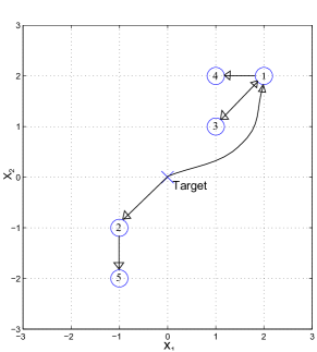
Figure 1: Communication topology and initial conditions.

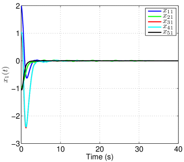
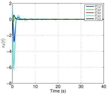
Figure 2: State trajectories for the first and the second state variable.

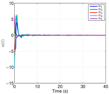
Figure 3: Control trajectories.

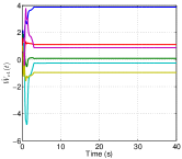
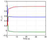
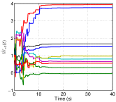
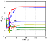
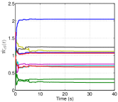
Figure 4: Value function weights.

Agent 1	Agent 2	Agent 3	Agent 4	Agent 5
$\begin{gathered}Q_{11}=I_{2},\>R_{1}=1,\\ Q_{13}=0.5\times I_{2}\end{gathered}$	$Q_{22}=I_{2}$, $R_{2}=1$	$\begin{gathered}Q_{33}=I_{2},\>R_{3}=1\\ Q_{31}=0.5\times I_{2}\end{gathered}$	$\begin{gathered}Q_{44}=I_{2},\>R_{4}=1\\ Q_{41}=0.1\times I_{2}\end{gathered}$	$\begin{gathered}Q_{54}=I_{2},\>R_{5}=1\\ Q_{52}=0.1\times I_{2}\end{gathered}$
$\begin{gathered}\sigma_{1}\left(\mathcal{E}_{1}\right)=[e_{11}^{2},\>e_{12}^{2},\\ e_{11}e_{12},\>e_{31}^{2},\>e_{32}^{2},\\ e_{31}e_{32}]\end{gathered}$	$\begin{gathered}\sigma_{2}\left(\mathcal{E}_{2}\right)=[e_{21}^{2},\>e_{22}^{2},\\ e_{21}e_{22}]\end{gathered}$	$\begin{gathered}\sigma_{3}\left(\mathcal{E}_{3}\right)=[e_{11}^{2},\>e_{12}^{2},\\ e_{11}e_{12},\>e_{31}^{2},\>e_{32}^{2},\\ e_{31}e_{32},\>e_{11}e_{31},\\ e_{12}e_{32},\>e_{11}e_{32},\\ e_{12}e_{31}]^{T}\end{gathered}$	$\begin{gathered}\sigma_{4}\left(\mathcal{E}_{4}\right)=[e_{11}^{2},\>e_{12}^{2},\\ e_{11}e_{12},\>e_{41}^{2},\>e_{42}^{2},\\ e_{41}e_{42},\>e_{11}e_{41},\\ e_{12}e_{42},\>e_{11}e_{42},\\ e_{12}e_{41}]\end{gathered}$	$\begin{gathered}\sigma_{5}\left(\mathcal{E}_{5}\right)=[e_{21}^{2},\>e_{22}^{2},\\ e_{21}e_{22},\>e_{51}^{2},\>e_{52}^{2},\\ e_{51}e_{52},\>e_{21}e_{51},\\ e_{22}e_{52},\>e_{21}e_{52},\\ e_{22}e_{51}]\end{gathered}$
$\begin{gathered}\eta_{a1}=0.1,\>\eta_{c1}=20,\\ \nu_{1}=0.0005\end{gathered}$	$\begin{gathered}\eta_{a2}=10,\>\eta_{c2}=20,\\ \nu_{2}=0.005\end{gathered}$	$\begin{gathered}\eta_{a3}=0.1,\>\eta_{c3}=20,\\ \nu_{3}=0.005\end{gathered}$	$\begin{gathered}\eta_{a4}=0.1,\>\eta_{c4}=20,\\ \nu_{4}=0.005\end{gathered}$	$\begin{gathered}\eta_{a5}=0.1,\>\eta_{c5}=10,\\ \nu_{5}=0.0005\end{gathered}$

Table I: Simulation parameters.

This section demonstrates the applicability of the developed technique. Consider the communication topology of five agents with unit pinning gains and edge weights with the initial configuration as shown in Figure 1. The dynamics of all the agents are chosen as [29]

$$\dot{x}_{i} =\left[\begin{array}[]{c}-x_{i1}+x_{i2}\\ -0.5x_{i1}-0.5x_{i2}(1-(cos(2x_{i1})+2)^{2})\end{array}\right]$$

$$+\left[\begin{array}[]{c}0\\ cos(2x_{i1})+2\end{array}\right]u_{i},$$

where $x_{i}\left(t\right)\triangleq[x_{i1}\left(t\right),x_{i2}\left(t\right)]^{T}\in\mathbb{R}^{2}$ is the state and $u_{i}(t)\in R$ is the control input. Table I summarizes the optimal control problem parameters, basis functions, and adaptation gains for the agents. In Table I, $e_{ij}$ denotes the $j^{th}$ element of the vector $e_{i}$.The value function and the policy weights are initialized equal to one, and the identifier weights are initialized as uniformly distributed random numbers in the interval $\left[-1,1\right]$. All the identifiers have five neurons in the hidden layer, and the identifier gains are chosen as

$$\Gamma_{wfi}=0.1\times I_{5},\>k_{fi}=600,\>\alpha_{fi}=300,$$

$$\gamma_{fi}=5,\>\beta_{1fi}=0.2.$$

An exponentially decreasing probing signal is added to the controllers to ensure PE. Figures 2 and 3 show the state and the control trajectories for all the agents demonstrating consensus to the origin. Note that agents 3, 4, and 5 do not have a communication link to the leader. In other words, agents 3, 4, and 5 do not know that they have to converge to the origin. The convergence is achieved via decentralized cooperative control. Figure 4 shows the evolution of the value function weights for the agents. Note that convergence of the weights is achieved. Figures 2-4 demonstrate the applicability of the developed method to cooperatively control a system of agents with partially unknown nonlinear dynamics on a communication topology. Two-hop local communication is needed to implement the developed method. Note that since the true weights are unknown, this simulation does not gauge the optimality of the developed controller. To gauge the optimality, a sufficiently accurate solution to the optimization problem will be sought via numerical optimization methods. The numerical solution will then be compared against the solution obtained using the proposed method.

VII Conclusion

This result combines graph theory and graph theory with the ACI architecture in ADP to synthesize approximate online optimal control policies for agents on a communication network with a spanning tree. NNs are used to approximate the policy, the value function, and the system dynamics. UUB convergence of the agent states and the weight estimation errors is proved through a Lyapunov-based stability analysis. Simulations are presented to demonstrate the applicability of the proposed technique to cooperatively control a group of five agents. Like other ADP-based results, this result hinges on the system states being PE. Furthermore, possible obstacles and possible collisions are ignored in this work. Future efforts will focus to resolve these limitations.

References

• [1] M. Lauer and M. A. Riedmiller, “An algorithm for distributed reinforcement learning in cooperative multi-agent systems,” in Proc. Int. Conf. Mach. Learn., ser. ICML ’00.   San Francisco, CA, USA: Morgan Kaufmann Publishers Inc., 2000, pp. 535–542. http://dl.acm.org/citation.cfm?id=645529.658113
• [2] L. Busoniu, R. Babuska, and B. De Schutter, “A comprehensive survey of multiagent reinforcement learning,” IEEE Trans. Syst. Man Cybern. Part C Appl. Rev., vol. 38, no. 2, pp. 156–172, 2008.
• [3] G. Wei$\beta$, “Distributed reinforcement learning,” Robot. Autom. Syst., vol. 15, no. 1-2, pp. 135 – 142, 1995, the Biology and Technology of Intelligent Autonomous Agents. http://www.sciencedirect.com/science/article/pii/092188909500018B
• [4] W. Cao, G. Chen, X. Chen, and M. Wu, “Optimal tracking agent: A new framework for multi-agent reinforcement learning,” in Proc. IEEE Int. Conf. Trust Secur. Priv. Comput. Commun., 2011, pp. 1328–1334.
• [5] K. Vamvoudakis and F. Lewis, “Multi-player non-zero-sum games: Online adaptive learning solution of coupled hamilton-jacobi equations,” Automatica, vol. 47, pp. 1556–1569, 2011.
• [6] R. S. Sutton and A. G. Barto, Reinforcement Learning: An Introduction.   Cambridge, MA, USA: MIT Press, 1998.
• [7] K. Vamvoudakis, F. L. Lewis, M. Johnson, and W. E. Dixon, “Online learning algorithm for stackelberg games in problems with hierarchy,” in Proc. IEEE Conf. Decis. Control, Maui, HI, Dec. 2012, pp. 1883–1889.
• [8] K. Vamvoudakis and F. Lewis, “Online neural network solution of nonlinear two-player zero-sum games using synchronous policy iteration,” in Proc. IEEE Conf. Decis. Control, 2010.
• [9] D. Vrabie and F. Lewis, “Integral reinforcement learning for online computation of feedback nash strategies of nonzero-sum differential games,” in Proc. IEEE Conf. Decis. Control, 2010, pp. 3066–3071.
• [10] M. Johnson, T. Hiramatsu, N. Fitz-Coy, and W. E. Dixon, “Asymptotic stackelberg optimal control design for an uncertain Euler-Lagrange system,” in Proc. IEEE Conf. Decis. Control, Atlanta, GA, 2010, pp. 6686–6691.
• [11] M. Johnson, S. Bhasin, and W. E. Dixon, “Nonlinear two-player zero-sum game approximate solution using a policy iteration algorithm,” in Proc. IEEE Conf. Decis. Control, 2011, pp. 142–147.
• [12] J. Wang and M. Xin, “Multi-agent consensus algorithm with obstacle avoidance via optimal control approach,” Int. J. Control, vol. 83, no. 12, pp. 2606–2621, 2010. http://www.tandfonline.com/doi/abs/10.1080/00207179.2010.535174
• [13] ——, “Distributed optimal cooperative tracking control of multiple autonomous robots,” Robotics and Autonomous Systems, vol. 60, no. 4, pp. 572 – 583, 2012. http://www.sciencedirect.com/science/article/pii/S0921889011002211
• [14] E. Semsar-Kazerooni and K. Khorasani, “Optimal consensus algorithms for cooperative team of agents subject to partial information,” Automatica, vol. 44, no. 11, pp. 2766 – 2777, 2008. http://www.sciencedirect.com/science/article/pii/S0005109808002719
• [15] K. G. Vamvoudakis, F. L. Lewis, and G. R. Hudas, “Multi-agent differential graphical games: Online adaptive learning solution for synchronization with optimality,” Automatica, vol. 48, no. 8, pp. 1598 – 1611, 2012. http://www.sciencedirect.com/science/article/pii/S0005109812002476
• [16] D. H. Shim, H. J. Kim, and S. Sastry, “Decentralized nonlinear model predictive control of multiple flying robots,” in Proc. IEEE Conf. Decis. Control, vol. 4, 2003, pp. 3621–3626.
• [17] L. Magni and R. Scattolini, “Stabilizing decentralized model predictive control of nonlinear systems,” Automatica, vol. 42, no. 7, pp. 1231 – 1236, 2006. http://www.sciencedirect.com/science/article/pii/S000510980600104X
• [18] P. Werbos, “Approximate dynamic programming for real-time control and neural modeling,” in Handbook of Intelligent Control: Neural, Fuzzy, and Adaptive Approaches, D. A. White and D. A. Sofge, Eds.   New York: Van Nostrand Reinhold, 1992.
• [19] S. Bhasin, R. Kamalapurkar, M. Johnson, K. Vamvoudakis, F. L. Lewis, and W. Dixon, “A novel actor-critic-identifier architecture for approximate optimal control of uncertain nonlinear systems,” Automatica, vol. 49, no. 1, pp. 89–92, 2013.
• [20] S. Khoo and L. Xie, “Robust finite-time consensus tracking algorithm for multirobot systems,” IEEE/ASME Trans. Mechatron., vol. 14, no. 2, pp. 219–228, 2009.
• [21] W. E. Dixon, A. Behal, D. M. Dawson, and S. Nagarkatti, Nonlinear Control of Engineering Systems: A Lyapunov-Based Approach.   Birkhauser: Boston, 2003.
• [22] R. Beard, G. Saridis, and J. Wen, “Galerkin approximations of the generalized Hamilton-Jacobi-Bellman equation,” Automatica, vol. 33, pp. 2159–2178, 1997.
• [23] K. Hornik, M. Stinchcombe, and H. White, “Universal approximation of an unknown mapping and its derivatives using multilayer feedforward networks,” Neural Netw., vol. 3, no. 5, pp. 551 – 560, 1990.
• [24] F. L. Lewis, R. Selmic, and J. Campos, Neuro-Fuzzy Control of Industrial Systems with Actuator Nonlinearities.   Philadelphia, PA, USA: Society for Industrial and Applied Mathematics, 2002.
• [25] R. M. Johnstone, C. R. Johnson, R. R. Bitmead, and B. D. O. Anderson, “Exponential convergence of recursive least squares with exponential forgetting factor,” in Proc. IEEE Conf. Decis. Control, vol. 21, 1982, pp. 994–997.
• [26] P. Ioannou and J. Sun, Robust Adaptive Control.   Prentice Hall, 1996.
• [27] H. K. Khalil, Nonlinear Systems, 3rd ed.   Prentice Hall, 2002.
• [28] G. Chen and F. L. Lewis, “Distributed adaptive tracking control for synchronization of unknown networked Lagrangian systems,” IEEE Trans. Syst. Man Cybern., vol. 41, no. 3, pp. 805–816, 2011.
• [29] K. Vamvoudakis and F. Lewis, “Online actor-critic algorithm to solve the continuous-time infinite horizon optimal control problem,” Automatica, vol. 46, pp. 878–888, 2010.