Effect of charged line defects on conductivity in graphene: numerical Kubo and analytical Boltzmann approaches

Abstract

Charge carrier transport in single-layer graphene with one-dimensional charged defects is studied theoretically. Extended charged defects, considered an important factor for mobility degradation in chemically-vapor-deposited graphene, are described by a self-consistent Thomas–Fermi potential. A numerical study of electronic transport is performed by means of a time-dependent real-space Kubo approach in honeycomb lattices containing millions of carbon atoms, capturing the linear response of realistic size systems in the highly disordered regime. Our numerical calculations are complemented with a kinetic transport theory describing charge transport in the weak scattering limit. The semiclassical transport lifetimes are obtained by computing scattered amplitudes within the second Born approximation. The transport electron–hole asymmetry found in the semiclassical approach is consistent with the Kubo calculations. In the strong scattering regime, the conductivity is found to be a sublinear function of electronic density and weakly dependent on the Thomas–Fermi screening wavelength. We attribute this atypical behavior to the extended nature of one-dimensional charged defects. Our results are consistent with recent experimental reports.

I Introduction

The isolation of graphene—the queen of two-dimensional materials due to its remarkable physical properties—by the exfoliation method has triggered intensive studies of its fundamental properties and has opened horizons for future technologies.Novoselov2004 ; Kats2007 ; Castro Netto review Since that time, various methods of graphene growth have been explored in order to make the fabrication process scalable; a prerequisite for developing graphene-based devices and technologies.Geim-Novos2007 Nowadays, several techniques are capable of producing high-quality, large-scale graphene. These include epitaxial graphene growth on SiC,de Heer2007 and chemical vapor deposition (CVD) of graphene on transition metal surfaces.Kim2009 The advantages of the latter method lie in its low cost, possibility to grow large graphene sheets (tens of inches), and ease of its transfer into other substrates.Bae2010 Currently, there is a strong motivation for exploring electronic and transport properties of CVD grown graphene because it represents one of the most promising materials for flexible and transparent electronics.

The studies of the transport properties of graphene are often focused on the fundamental question: what limits a charge carrier mobility in it? As far as CVD-grown graphene is concerned, it is believed that its transport properties are strongly affected by the presence of charged line defects.FerreiraEPL Usually, the growth of graphene by the CVD-method requires to use metal surfaces with hexagonal symmetry, such as the (111) surface of cubic or the (0001) surface of hexagonal crystals.Krasheninnikov2011 The mismatch between the metal-substrate and graphene causes the strains in the latter, reconstructs the chemical bonds between the carbon atoms and results in formation of two-dimensional (2D) domains of different crystal orientations separated by one-dimensional defects.Krasheninnikov2011 ; Jeong2008 ; Yazyev2010 ; Malola2010 The nucleation of the graphene phase takes place simultaneously at different places, which leads to the formation of independent 2D domains matching corresponding grains in the substrate. A line defect appears when two graphene grains with different orientations coalesce; the stronger the interaction between graphene and the substrate, the more energetically preferable the formation of line defects is. These line defects accommodate localized states trapping the electrons, originating lines of immobile charges that scatter the Dirac fermions in graphene.

It is well established that the presence of grains and grain boundaries in three-dimensional polycrystalline materials can strongly affect their electronic and transport properties. Hence, in principle, the role of such structures in 2D materials, such as graphene, can be even more important because even a single line defect can divide and disrupt the crystal.Krasheninnikov2011 A series of recent control experimentsSong2012 ; Li2009 strongly indicate that line defects are responsible for lower carrier mobility in CVD-grown graphene in comparison to the exfoliated samples.Morozov2008 ; Bolotin2008 ; Du2008 We note in passing that one-dimensional (1D) defects have been observed not only in experimental studies on CVD growth of graphene films, for instance, on Cu,Li2009 Ni,Lahiri2010 Ir,Coraux2008 but also in single graphene layer after electron irradiationHashimoto2004 and in highly oriented pyrolytic graphite surface.Cervenka2009 Possible applications include: valley filtering based on scattering off line defects,Gunlycke2011 ferromagnetic ordering in line defects,Okada2011 ; Kou2011 enhancement of electron transportKindermann2010 or chemical reactivityBotello2011 due to induced extra conducting channels and localized states along the line, quantum channels controlled by tuning of the gate voltage embedded below the line defect,SongPRB2012 and correlated magnetic states in extended defects.Alexandre2012

Several theoretical studies have been recently reported addressing transport properties of graphene with a single graphene boundaryYazyevNature ; Liwei ; Peres or polycrystalline graphene with many domain boundaries.Tuan2013 On the other hand, much less attention has been paid to the effect of charge accumulation at these boundaries due to self-doping. Transport properties of graphene with 1D charged defects has been studied in Ref. FerreiraEPL, using the Boltzmann approach within the first Born approximation. It has been demonstrated previously that such approximation is not always applicable for the description of electron transport in graphene even at finite (non-zero) electronic densities.Klos2010 ; Ferreira ; HengyiXu2011 ; Radchenko In the present work we investigate the impact of extended charged defects in the transport properties of graphene by an exact numerical approach based on the time-dependent real-space quantum Kubo methodRoche_SSC ; Roche1997 ; Triozon2002 ; Triozon2004 ; Markussen ; Ishii ; Yuan10 ; Ferreira ; Leconte11 ; Trambly ; Lherbier08100 ; Lherbier08101 ; Lherbier11 ; Radchenko which is especially suited to treat large graphene systems with dimensions approaching realistic systems containing millions of atoms. Our numerical calculations are complemented with a semi-classical treatment going beyond the first Born approximation, describing the transport properties in the weak scattering regime.

The paper is organized as follows. The numerical models (tight-binding approximation and Kubo approach) and obtained results are presented in Sec. II. In Sec. III we study the impact of extended charged defects within kinetic transport theory. Here, the general expression for the scattering amplitude for massless fermions within the second Born approximation is derived and used to obtain the semiclassical conductivity and the transport electron–hole asymmetry. The approaches in Secs. II and III provide information about transport dominated by 1D charged defects in distinct regimes. Section IV presents the conclusions of our work. Details of numerical calculations and analytic derivations are given in the Appendixes.

II Tight-binding model and time-dependent real-space Kubo–Greenwood formalism

In this section, we introduce to the basis of the tight-binding approximation as well as the Kubo–Greenwood approach and also present numerical results obtained within the framework of these models.

II.1 Basics

To model electron dynamics in graphene, we use a standard $p$-orbital nearest neighbor tight-binding Hamiltonian defined on a honeycomb latticeCastro Netto review ; Peres_review ; DasSarma_review

$$\hat{H}=-u\sum_{i,i^{\prime}}c_{i}^{\dagger}c_{i^{\prime}}+\sum_{i}V_{i}c_{i}^{\dagger}c_{i},$$ (1)

where $c_{i}^{\dagger}$ and $c_{i}$ are the standard creation and annihilation operators acting on a quasiparticle on the site $i$. The summation over $i$ runs over the entire graphene lattice, while $i^{\prime}$ is restricted to the sites next to $i$; $u=2.7$ eV is the hopping integral for the neighboring C atoms $i$ and $i^{\prime}$ with distance $a=0.142$ nm between them, and $V_{i}$ is the on-site potential describing impurity (defect) scattering.

Since line defects can be thought as lines of reconstructed point defects,Jeong2008 ; Krasheninnikov2011 ; Yazyev2010 ; Malola2010 we model a 1D defect as point defects oriented along a fixed direction (corresponding to the line direction) in the honeycomb lattice. The electronic effective potential for a charged line within the Thomas–Fermi approximation was first obtained in Ref. FerreiraEPL, (see also Appendix A); if there are $N_{\text{lines}}$ such charged lines in a graphene lattice, the effective scattering potential reads as

$$V_{i}= \sum_{j=1}^{N_{\text{lines}}}U_{j}[-\text{cos}(q_{\mathrm{\textrm{TF}}}x_{ij})\text{Ci}(q_{\textrm{TF}}x_{ij})+$$

$$+\text{sin}(q_{\textrm{TF}}x_{ij})(\pi/2-\text{Si}(q_{\textrm{TF}}x_{ij}))],$$ (2)

where $U_{j}$ is a potential height, $x_{ij}$ is a distance between the site $i$ and the $j$-th line, $q_{\textrm{TF}}=e^{2}k_{F}/(\pi\varepsilon_{0}\varepsilon_{\textrm{r}}\hbar v_{F})$ is the Thomas–Fermi wavevector defined by the electron Fermi velocity $v_{F}=3ua/(2\hbar)$ and the Fermi momentum $k_{F}=\sqrt{\pi|n_{e}|}$ (related to the electronic carrier density $n_{e}$ controlled applying the back-gate voltage). Here, $-e<0$ denotes the electron charge. The Thomas–Fermi wavevector is also commonly expressed as a function of graphene’s structure constant $\alpha_{\textrm{g}}\equiv e^{2}k_{F}/(4\pi\varepsilon_{0}\varepsilon_{\textrm{r}}\hbar v_{F})$ according to $q_{\textrm{TF}}=4\alpha_{\textrm{g}}k_{F}$. We consider two cases: symmetric, $V\gtrless 0$, and asymmetric, $V>0$, potentials, where $U_{j}$ are chosen randomly in the ranges $\left[-\triangle,\triangle\right]$ and $\left[0,\triangle\right]$, respectively, with $\triangle$ being the maximal potential height. In order to simplify numerical calculations, we fit the potential (2) by the Lorentzian function

$$V_{i}=\sum_{j=1}^{N_{\text{lines}}}U_{j}(A/(B+Cx_{ij}^{2}))$$ (3)

as described in Appendix A. A typical shape of the effective potential for both symmetric and asymmetric cases is illustrated in Fig. 1.

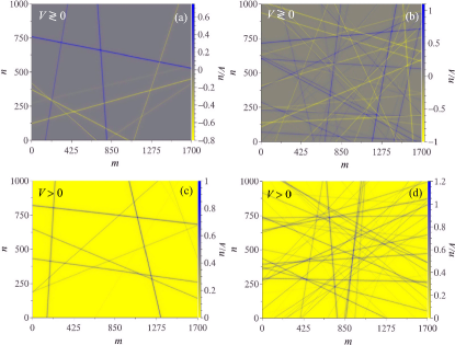
Figure 1: (Color online) Effective symmetric [(a),(b)] and asymmetric [(c),(d)] potentials describing one of the possible configurations of 10 (left) and 50 (right) line defects in graphene sheet of the size $m\times n=1700\times 1000$ sites corresponding to $210\times 210$ nm. Maximal potential height $\triangle=0.25u$.

II.2 Time-dependent real-space Kubo method

To calculate numerically the dc conductivity $\sigma$ of graphene sheets with 1D charged defects, the real-space order-$N$ numerical implementation within the Kubo–Greenwood formalism is employed, where $\sigma$ is extracted from the temporal dynamics of a wave packet governed by the time-dependent Schrödinger equation.Roche_SSC ; Roche1997 ; Trambly ; Triozon2002 ; Triozon2004 ; Yuan10 ; Markussen ; Ishii ; Leconte11 ; Lherbier08100 ; Lherbier08101 ; Lherbier11 ; Tuan2013 This is a computationally efficient method scaling with a number of atoms in the system $N$, and thus allowing treating very large graphene sheets containing many millions of C atoms.

A central quantity in the Kubo–Greenwood approach is the mean quadratic spreading of the wave packet along the $x$-direction at the energy $E$, $\Delta\hat{X}^{2}(E,t)=\bigl{\langle}\hat{(X}(t)-\hat{X}(0))^{2}\bigr{\rangle}$, where $\hat{X}(t)=\hat{U}^{\dagger}(t)\hat{X}\hat{U}(t)$ is the position operator in the Heisenberg representation, and $\hat{U}(t)=e^{-i\hat{H}t/\hbar}$ is the time-evolution operator. Starting from the Kubo–Greenwood formula for the dc conductivityMadelung

$$\sigma=\frac{2\pi\hbar e^{2}}{\Omega}\text{Tr}[\hat{v}_{x}\delta(E-\hat{H})\hat{v}_{x}\delta(E-\hat{H})],$$ (4)

where $\hat{v}_{x}$ is the $x$-component of the velocity operator, $E$ is the Fermi energy, $\Omega$ is the area of the graphene sheet, and factor 2 accounts for the spin degeneracy, the conductivity can then be expressed as the Einstein relation,

$$\sigma\equiv\sigma_{xx}=e^{2}\tilde{\rho}(E)\lim_{t\rightarrow\infty}D(E,t),$$ (5)

where $\tilde{\rho}(E)=\rho/\Omega=\textrm{Tr}[\delta(E-\hat{H})]/\Omega$ is the density of sates (DOS) per unit area (per spin), and the time-dependent diffusion coefficient $D(E,t)$ relates to $\Delta\hat{X}^{2}(E,t)$ according to

$$D(E,t)= \frac{\bigl{\langle}\Delta\hat{X}^{2}(E,t)\bigr{\rangle}}{t}$$

$$= \frac{1}{t}\frac{\text{Tr}[\hat{(X}_{H}(t)-\hat{X}(0))^{2}\delta(E-\hat{H})]}{\text{Tr}[\delta(E-\hat{H})]}.$$ (6)

It should be noted that in the present study we are interested in the diffusive transport regime when the diffusion coefficient reaches its maximum. Therefore, following Refs. Leconte11, and Lherbier12, , we replace in Eq. (5) $\lim_{t\rightarrow\infty}D(E,t)\rightarrow D_{\max}(E),$ such that the dc conductivity is defined as

$$\sigma=e^{2}\tilde{\rho}(E)D_{\max}(E).$$ (7)

Note that in most experiments, the conductivity is measured as a function of electron density $n_{e}$. We calculate the electron density as $n_{e}(E)\equiv n_{e}=\int_{-\infty}^{E}\tilde{\rho}(E)dE-n_{\text{ions}},$ where $n_{\text{ions}}=3.9\cdot 10^{15}$ cm^-2 is the density of the positive ions in the graphene lattice compensating the negative charge of the $p$-electrons [note that for the ideal graphene lattice at the neutrality point $n(E)=0$]. Combining the calculated $n_{e}(E)$ with $\sigma(E)$ given by Eq. (7) we obtain the required dependence of the conductivity $\sigma=\sigma(n_{e})$.

II.3 Numerical results

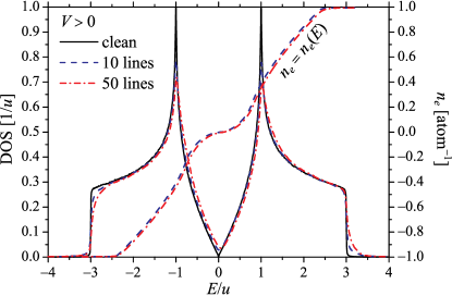
Figure 2: (Color online) Density of states (DOS) and the relative charge carrier concentration $n_{e}$ (the number of electrons per C atom) vs. the energy $E$ for 10 and 50 positively-charged line defects described by the symmetric potential potential with $\triangle=0.25u$.

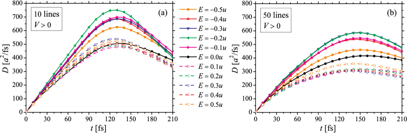
Figure 3: (Color online) Time-dependent diffusion coefficient at different energies for 10 (a) and 50 (b) positively-charged line defects ($\triangle=0.25u$).

This subsection presents numerical results for the dc conductivity calculated using the time-dependent real space Kubo–Greenwood formalism within the tight-binding model. We compute the density dependence of the conductivity for graphene sheets with 10 and 50 lines in $1700\times 1000$ lattice. This approximately corresponds to a relative concentration of point defects of respectively 1% and 5%. We model the potential due to lines of charges by the Lorentzian function, Eq. (3), where we set $q_{\textrm{TF}}a=0.1$, which corresponds to typical electron densities $|n_{e}^{\exp}|\sim 5\cdot 10^{-5}$ atom^-1 ($|n_{e}^{\exp}|\sim 2\cdot 10^{11}$ cm^-2), see Fig. 1. It should be noted that $q_{\textrm{TF}}$ is not a constant but weakly density dependent ($q_{\textrm{TF}}\propto\sqrt{|n_{\textrm{e}}|}$). Quite remarkably, the obtained results for the conductivity remain practically unchanged when we use different $q_{\textrm{TF}}$ corresponding to representative electron densities considered in the present study, $1\cdot 10^{-5}\lesssim|n_{e}|\lesssim 5\cdot 10^{-5}$ atom^-1. In Appendix B we present results of more elaborated self-consistent calculations where we use the exact shape of the Thomas–Fermi potential [i.e., Eq. (2) instead of Eq. (3)] and take into account the density dependence of $q_{\textrm{TF}}$. We found that even for a single charged line embedded in a graphene sheet, the dependence $\sigma=\sigma(n_{e})$ calculated for the exact self-consistent (i.e., $n_{e}$-dependent) potential (2) exhibits qualitatively and quantitatively the same sublinear behavior as in the simulations with the fixed Thomas–Fermi wavevector ($q_{\textrm{TF}}a=0.1$) and with $V_{i}$ given by the Lorentzian function Eq. (3). The same conclusion holds for samples with 10 and 50 lines. Because of this in what follows we will discuss the results for the case of the Lorentzian potential at the fixed $q_{\textrm{TF}}$.

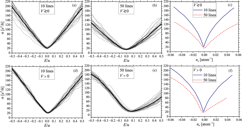
Figure 4: (Color online) Conductivity as a function of energy $E$ [(a),(b),(d),(e)] and relative electron density $n$ [(c),(f)] for different configurations of 10 and 50 positively-charged 1D defects ($\triangle=0.25u$). Conductivities in (c) and (f) are averaged over 20 different realizations in (a), (b), and (d), (e).

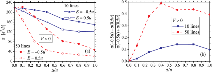
Figure 5: (Color online) (a) The conductivity and and relative (b) values of conductivities for two symmetrical (with respect to the Dirac point) energies as the functions of positive (asymmetric) potential $V\sim U\in[0,\triangle]$.

Figure 2 shows the electron density $n_{e}=n(E)$ and the DOS in a graphene sheet with different number of charged lines. The calculated dependencies are very much similar to those for clean graphene and for graphene with a long-range Gaussian potential.Yuan10 ; Radchenko (Note that the DOS of graphene with short-range strong scatterers exhibits an impurity peak in the vicinity of neutrality point.)Pereira06 ; peres2006 ; Yuan10 ; Ferreira ; Radchenko For both symmetric (not shown here) and asymmetric potentials, the DOS does not reach zero at the Dirac point, and the asymmetric potential (in contrast to the symmetric one) leads to electron–hole asymmetry in the DOS.

The time dependence of the diffusion coefficient at different energies for the case of a symmetric potential corresponding to 10 and 50 positively charged line defects is shown in Fig. 3. [Diffusivity curves for the case of asymmetric potential (not shown here) exhibit similar behavior.] After an initial linear increase corresponding to the ballistic regime, the diffusion coefficient reaches its maximum at $t\thickapprox 130$ and 150 fs for 10 and 50 lines, respectively. These values of $D=D_{\max}$ are used to calculate $\sigma$ according to Eq. (7). For times $t\gtrsim 150$, $D(t)$ decreases due to the localization effects. Similar temporal behavior of the diffusion coefficient was established earlier for different types of scatterers in graphene including long-range Gaussian and short-range potentials.Leconte11 ; Lherbier12 ; Radchenko

In Fig. 4 we show the density dependence of the conductivity of graphene sheets with linear defects for the cases of symmetric and asymmetric potentials. The obtained dependencies show following features.

First, the averaged conductivities exhibit a pronounced sublinear density dependence, see Figs. 4(c) and 4(f). Our numerical calculations are consistent with the recent experimental results for the CVD-grown grapheneKim2009 ; Song2012 ; Tsen2010 that also exhibit sublinear density dependence. This provides an evidence in support that the line defects represent the dominant scattering mechanism in CVD-grown graphene.FerreiraEPL ; Kim2009 ; Song2012 Note that the calculated sublinear density dependence for the case of linear defects is quite different from the case of short- and long-range point scatterers where the numerical calculations show a density dependence which is close to linear.Lewenkopf ; Klos2010 ; Yuan10 ; Ferreira ; Radchenko

Second, the conductivities of samples with different impurity configurations exhibit significant variations between each other, see Figs. 4(a)–4(b), 4(d)–4(e). This is in strong contrast to the case of short- and long-range point scatterers where corresponding conductivities of samples of the same size and impurity concentrations practically did not show any noticeable differences for different impurity configurations.Radchenko We attribute this to the fact that in contrast to point defects, the line defects are characterized not only by their positions, but also by directions (orientations) and their intersections as well. Such additional characteristics result in much more possible distributions of the potential which, in turn, leads to the differences in the conductivity curves.

Third, for the symmetric potential the conductivity curves are symmetric with respect to the neutrality point, while the asymmetric one shows the asymmetry of the conductivity, c.f., Figs. 4(c) and 4(f). Such asymmetry between the holes and electrons have been also reported in many transport calculations for graphene with point defects, for instance in Refs. Lherbier08101, ; Robinson, ; Wehling, ; Leconte11, ; Ferreira, and Radchenko, . For a closer inspection of the effect of asymmetry we plotted the conductivities for representative energies $E=\pm 0.5u$, Fig. 5(a) as well as their relative differences $\frac{\sigma(-E)-\sigma(E)}{\sigma(-E)+\sigma(E)}$ as a function of the potential strength $\Delta$, Fig. 5(b). The relative conductivity difference exhibits a linear behavior for $\Delta\lesssim 0.4u$ followed by saturation for larger values of $\Delta$. A comparison of the obtained numerical results with the analytic predictions in the weak scattering regime will be given in what follows.

We conclude this section by noting that conductivity of large CVD-grown graphene polycrystalline samples with disordered grain boundaries was calculated by Tuan et al.Tuan2013 using the same time-dependent real-space Kubo method. In contrast to the long-range Thomas–Fermi potential considered here, the onsite potential in Ref. Tuan2013, is set to zero and the scattering is due to grain boundaries separating domains with different crystallographic orientations. Even though this study did not discuss a functional dependence of the conductivity, a visual inspection of the obtained results reveals an approximate linear dependence of the conductivity on the Fermi energy, which is consistent with our results. Moreover, the conductance of graphene with several types of domain boundaries has also been shown to be a linear function of the Fermi energy.Peres We therefore speculate that the linear energy dependence (and thus the sublinear density dependence) of the conductivity is related to scattering off extended defects. More systematic studies of scattering for different forms of potentials are needed in order to clarify this question.

III Boltzmann approach

III.1 Formalism

In this section we tackle the problem of dc transport in graphene with 1D charged defects by means of semiclassical Boltzmann theory. We would like to stress that the full quantum calculations of Sec. II and semiclassical kinetic theory provide complementary information about electronic transport; while the former is more suitable to handle highly disordered systems or strong scattering regime (given practical computational limitations),comment semi-classical approaches yield an accurate picture of charge transport for dilute disorder and are often limited to the weak scattering regime (an exception being resonant scattering which can be treated non-perturbatively).Ferreira Here, the dimensionless parameter $\beta\equiv|\Delta|L/(\hbar v_{F}$), with $L$ of the order of the system size, defines the onset of weak scattering regime, i.e., $\beta\ll 1$. Note that the simulations of the previous section have $\beta\gtrsim 10^{2}$, and therefore fall well inside the strong scattering regime.

The effective potential of a charged line is long-ranged and hence we neglect intervalley scattering. Within the Dirac cone approximation, the semiclassical dc conductivity of graphene at zero temperature is given byCastro Netto review ; Peres_review ; DasSarma_review ; Ferreira

$$\sigma=\frac{ge^{2}}{2h}k_{F}v_{F}\tau(k_{F})\,.$$ (8)

In the above, the factor $g=4$ accounts for spin and valley degeneracies, and $\tau(k_{F})$ is the transport scattering time at the Fermi surface

$$\tau(k_{F})=\left[n_{l}v_{F}\int d\theta(1-\cos\theta)|f(\theta)|^{2}\right]^{-1}\,,$$ (9)

where $f(\theta)$ is the scattering amplitude at an angle $\theta$ and $n_{l}$ stands for the (areal) density of charged lines.

In this work we compute the scattering amplitudes in the second Born approximation (SBA) with respect to the scattering potential $V(\boldsymbol{r})$. This allows us to improve over the commonly employed first Born approximation (FBA) by capturing the non-trivial effect of electron–hole asymmetry; see Fig. 6. In the Appendix C we show that the SBA scattering amplitude for 2D massless fermions is given by

$$f_{\textrm{SBA}}(\theta) = \frac{\Xi(\theta)}{v_{F}\hbar}\sqrt{\frac{k}{8\pi}}\left\{\tilde{V}(\mathbf{q})+\int\frac{d^{2}\mathbf{p}}{\left(2\pi\right)^{2}}\tilde{V}(\mathbf{k}^{\prime}-\mathbf{p})\times\right.$$ (10)

$$\left.\langle u_{\mathbf{k}}|G_{0}(\mathbf{p})|u_{\mathbf{k}}\rangle\tilde{V}(\mathbf{p}-\mathbf{k})\right\},$$

where $\tilde{V}(\mathbf{q})$ denotes the 2D Fourier transform of the scattering potential energy of a charged line $\tilde{V}(\mathbf{q})=\int d^{2}\mathbf{r}e^{-i\mathbf{q}\cdot\mathbf{r}}V(\mathbf{r})$, and $G_{0}(\mathbf{p})$ is the 2D Dirac fermion propagator for particles with energy $E_{F}=sv_{F}\hbar k_{F},$ i.e.,

$$G_{0}(\mathbf{p})=\frac{1}{\hbar^{2}v_{F}^{2}}\frac{E_{F}+\hbar v_{F}\boldsymbol{\sigma}\cdot\mathbf{p}}{k_{F}^{2}-p^{2}+is0^{+}}\,.$$ (11)

The symbol $s=\pm 1$ distinguishes between electrons and holes, that is, $s\equiv\textrm{sign}(E_{F})$. $\mathbf{k}$ is the wavevector of the incident electron, $\hbar\mathbf{q}=\hbar(\mathbf{k}^{\prime}-\mathbf{k})$ is the transferred momentum ($\mathbf{k}^{\prime}$ stands for the ‘out’ wavevector), $\theta=\angle(\mathbf{k}^{\prime},\mathbf{k})$ is the scattering angle, $|u_{\mathbf{k}}\rangle=2^{-1/2}(1,\>se^{i\theta_{\mathbf{k}}})^{T}$ is the Dirac spinor for scattered particles, and the form factor $\Xi(\theta)=1+e^{i\theta}$ comes from graphene’s sublattice symmetry and precludes carriers from back-scatter. Without loss of generality, in what follows, we consider incident carriers propagating along the $x$-direction, $\mathbf{k}=k_{F}e_{\boldsymbol{x}}$.

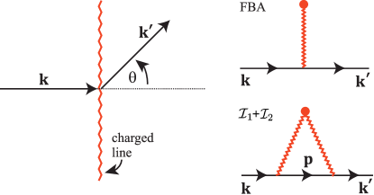
Figure 6: (Color online) Schematic picture showing a scattering event and Feynman scattering diagrams considered in this work. The circle signifies the extended charged defect with charge density $\lambda$ and the zigzag (solid) line denotes the scattering potential (bare propagator). The transport relaxation rate is $\mathcal{O}(\lambda^{2})$ in the FBA approximation (top diagram) and $\mathcal{O}(\lambda^{3})$ in the SBA (bottom diagram).

The first term inside brackets in Eq. (10) is proportional to the Fourier transform of the scattering potential evaluated at the transferred momentum $\hbar\mathbf{q}$, that is, the familiar FBA scattering amplitude. The remaining terms result from the next-order correction to the FBA and require the calculation of two integrals, namely

$$\mathcal{I}_{1}\equiv\hbar v_{F}k_{F}\int\frac{d^{2}\mathbf{p}}{\left(2\pi\right)^{2}}\tilde{V}(\mathbf{k}^{\prime}-\mathbf{p})g(\mathbf{p})\tilde{V}(\mathbf{p}-\mathbf{k}),$$ (12)

$$\mathcal{I}_{2}\equiv\int\frac{d^{2}\mathbf{p}}{\left(2\pi\right)^{2}}\tilde{V}(\mathbf{k}^{\prime}-\mathbf{p})[\hbar v_{F}\mathbf{p}\cdot\boldsymbol{e}_{x}]g(\mathbf{p})\tilde{V}(\mathbf{p}-\mathbf{k}).$$ (13)

In writing these equations, we have defined the function

$$g(\mathbf{p})=(\hbar v_{F})^{-2}\left(k_{F}^{2}-p^{2}+is0^{+}\right)^{-1}\,.$$ (14)

The scattering potential of an infinite line with density charge $\rho=\lambda\delta(x)\delta(z)$ was derived by some of the authors in Ref. FerreiraEPL, and is given by

$$\tilde{V}(\boldsymbol{q})=2\pi\delta(q_{y})\frac{\Delta}{|q_{x}|+q_{\textrm{TF}}}\,,$$ (15)

where the parameter with units of energy $\Delta$ relates to the charge density of a line $\lambda$ according to $\Delta=s\lambda e/(2\varepsilon_{0})$ (in vacuum); note that the absolute value of $\Delta$ coincides with the definition of $\Delta$ as given in Sec. II.1. The delta function in Eq. (15) reflects momentum conservation along the direction defined by the line. For completeness, a derivation of this result is provided in Appendix A.

In order to mimick the effect of lines with finite length we have to modify Eq. (15) as to allow for momentum transfer to occur along both spatial directions. To this end, we introduce a length scale associated with the line’s average length $L$. In the limit of small $k_{F}L$, we replace $2\pi\delta(q_{y})\rightarrow L$,finite_line as to obtain

$$\tilde{V}_{L}(\boldsymbol{q})\equiv\frac{L\Delta}{|q_{x}|+q_{\textrm{TF}}}\,.$$ (16)

We use this potential as a toy model for describing transport for dilute concentrations of lines of charge. The particularly simple form of $\tilde{V}_{L}(\boldsymbol{q})$ allows for an exact calculation of scattering amplitudes, as shown in what follows.

III.2 First Born approximation

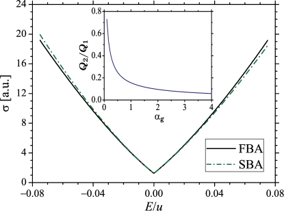
Figure 7: (Color online) Semi-classical dc conductivity at fixed Thomas–Fermi wavevector as a function of Fermi energy in the weak scattering regime with $\beta=0.08$ and $q_{\textrm{TF}}a=0.01$. Inset: The ratio $Q_{2}(\alpha_{\textrm{g}})/Q_{1}(\alpha_{\textrm{g}})$ determining the amount of transport electron–hole asymmetry is plotted as function of graphene’s effective structure factor $\alpha_{\textrm{g}}$.

The FBA provides a good approximation to transport scattering rates for 1D charged defects with $|\Delta|\ll\hbar v_{F}L^{-1}$ ($\beta\ll 1$). Within the FBA we retain only the first term in Eq. (10). The transport relaxation rate

$$[\tau_{\textrm{FBA}}(k_{F})]^{-1} = n_{l}v_{F}\frac{L^{2}\Delta^{2}k_{F}}{8\pi v_{F}^{2}\hbar}\int_{0}^{2\pi}d\theta(1-\cos\theta)\times$$ (17)

$$|\Xi(\theta)|^{2}[k_{F}(1-\cos\theta)+q_{\textrm{TF}}]^{-2}\,,$$

can be computed analytically and leads to the following result

$$\tau_{\textrm{FBA}}(k_{F})=\frac{1}{v_{F}n_{l}\beta^{2}}\frac{2k_{F}\sqrt{q_{\textrm{TF}}(2k_{F}+q_{\textrm{TF}})}}{k_{F}+q_{\textrm{TF}}-\sqrt{q_{\textrm{TF}}(2k_{F}+q_{\textrm{TF}})}}\,.$$ (18)

Invoking the semi-classical expression for the dc conductivity Eq. (8) and the relation $q_{\textrm{TF}}=4\alpha_{\textrm{g}}k_{F}$, we conclude that $\sigma$ is proportional to $k_{F}^{2}$, according to

$$\sigma=\frac{4e^{2}}{h}\frac{f(4\alpha_{\textrm{g}})}{n_{l}\beta^{2}}k_{F}^{2}\,,$$ (19)

with $f(x)=g(x)/[1+x-g(x)]$ and $g(x)=\sqrt{x(2+x)}$. The dependence of Eqs. (18)–(19) on the Fermi wavevector could be anticipated from the form of the effective potential in Fourier space, Eq. (16); as $\tilde{V}\propto k_{F}^{-1}$, the relaxation time must be proportional to $k_{F}$ at all orders in the Born series, implying $\sigma\propto k_{F}^{2}\propto|n_{e}|$. In other words, higher order corrections to the FBA renormalize the mobility of carriers $\mu\equiv\sigma/|n_{e}|$, while preserving the overall dependence of $\sigma$ and $\mu$ on the Fermi energy. This property is specific to the potential $\tilde{V}_{L}(\boldsymbol{q})$ and therefore is not expected to hold in models of extended charged defects beyond the limit of small $k_{F}L$.

We briefly discuss how the FBA conductivity compares with the results reported earlier in Fig. 4. The solid line in Fig. 7 shows the FBA conductivity at fixed Thomas–Fermi wavevector, i.e., $q_{\textrm{TF}}a=0.01$. In this case, the function $f(4\alpha_{\textrm{g}})$ is no longer constant and the functional dependence of $\sigma$ with $k_{F}$ is changed to linear at small energies, hence resembling the Kubo results. However, this comparison should not be pushed too far; note that the slope of the FBA $\sigma$ versus $E$ curve depends linearly on $q_{\textrm{TF}}$, and therefore Eq. (19) (and hence the quadratic dependence) is recovered when the self-consistent relation $q_{\textrm{TF}}=4\alpha_{\textrm{g}}k_{F}$ is used. In fact,

$$\sigma(k_{F},q_{\textrm{TF}})=\frac{4e^{2}}{h}\frac{q_{\textrm{TF}}k_{F}}{n_{l}\beta^{2}},\quad k_{F}\ll q_{\textrm{TF}}\,.$$ (20)

whereas the Kubo simulations show $\sigma\propto k_{F}$ independently on $q_{\textrm{TF}}$ in a wide range of energies. The latter behavior does not occur in the weak scattering regime described here.

III.3 Second Born approximation: electron–hole asymmetry

A large sensitivity to the carriers polarity in transport dominated by charged lines is borne out in the numerical simulations of Sec. II. Here, we describe this effect from the point of view of semiclassical transport theory. According to the Fermi golden rule the transport relaxation rate depends on the modulus square of the scattering potential; hence, in FBA approximation, opposite charges $\pm e$ have the same scattering amplitudes and hence cannot be distinguished. As observed earlier, the dependence of $\sigma$ on the carriers polarity can be captured by retaining the next term in the Born series for the scattering amplitude $f(\theta)$—the SBA bottom diagram in Fig. 6.

We compute the transport electron–hole asymmetry, defined as

$$\delta\equiv\left|\frac{\sigma_{\textrm{dc}}-\sigma_{\textrm{dc}}^{*}}{\sigma_{\textrm{dc}}+\sigma_{\textrm{dc}}^{*}}\right|\,,$$ (21)

with $\sigma_{\textrm{dc}}^{*}\equiv\left.\sigma_{\textrm{dc}}\right|_{e\rightarrow-e}=\left.\sigma_{\textrm{dc}}\right|_{\Delta\rightarrow-\Delta}$. In the weak scattering regime, $L|\Delta|\ll\hbar v_{F}$, the asymmetry parameter is proportional to the ratio of the bottom to the top diagrams in Fig. 6. Explicitly,

$$\delta=\frac{2\,\textrm{sign}\Delta\,\textrm{Re}\int d\theta|\Xi(\theta)|^{2}(1-\cos\theta)[\mathcal{I}_{1}+\mathcal{I}_{2}]\tilde{V}(q_{\theta})}{\int d\theta|\Xi(\theta)|^{2}(1-\cos\theta)|\tilde{V}(q_{\theta})|^{2}}\,,$$ (22)

where $q_{\theta}=2k_{F}\sin(\theta/2)$ is the transferred momentum in elastic scattering events. Remark that $\mathcal{I}_{1(2)}$ in Eq. (22) depend on the angle $\theta$ through the wavevector $\mathbf{k}^{\prime}$ [c.f., Eqs. (12)–(13)]. The derivation of this and related results is given in Appendix D.

Inserting the potential energy of a charged line Eq. (16) into the above expression and performing the angular integration yields

$$\delta\approx\left|\frac{\Delta L}{\hbar v_{F}}\right|\frac{Q_{2}(\alpha_{\textrm{g}})}{Q_{1}(\alpha_{\textrm{g}})}\,.$$ (23)

The explicit form of the functions $Q_{1}(\alpha_{\textrm{g}})$ and $Q_{2}(\alpha_{\textrm{g}})$ is given in Eqs. (85) and (89), respectively. For the toy model of a charged line considered here [Eq. (16)], cross sections are proportional to $k_{F}^{-1}$ at all orders, implying that the asymmetry parameter $\delta$ is insensitive to the Fermi energy. Indeed, the electron–hole asymmetry depends only on the magnitude of the Thomas–Fermi screening through the effective graphene’s structure constant, $\alpha_{\textrm{g}}$. In vacuum, $\alpha_{\textrm{g}}\approx 2.5$, and the evaluation of Eq. (23) yields $\delta\approx 0.08\cdot\beta$. The ratio $Q_{2}/Q_{1}$ is found to be very sensitive to the effective screening length of a charged line (refer to inset of Fig. 7); for $q_{\textrm{TF}}\gg k_{F}$ ($\alpha_{\textrm{g}}\gg 1$) screening is very efficient and electron–hole asymmetry is negligible, whereas for $q_{\textrm{TF}}\lesssim k_{F}$ ($\alpha_{\textrm{g}}\lesssim 1$) the ratio $Q_{2}/Q_{1}$ can assume large values leading to an enhancement of the asymmetry parameter $\delta$.

The transport electron–hole asymmetry in scattering events reflects into a decrease (increase) of the SBA transport relaxation time with respect to the FBA result for positive (negative) Fermi energy. In fact, by expanding the SBA transport relaxation rate Eq. (9) in the small parameter $\beta$, we find

$$\tau(k_{F})=\left[1-s\delta(\alpha_{\textrm{g}})+\mathcal{O}(\beta^{2})\right]\tau_{\textrm{FBA}}(k_{F}).$$ (24)

This result shows that the effect of second term in the Born series (bottom diagram in Fig. 6) is to renormalize the transport relaxation time according to the carriers polarity, $s$, and screening strength $\alpha_{\textrm{g}}$. This behavior is qualitatively consistent with the numerical Kubo simulations (see Fig. 4, for instance). In order to make the comparison between the semiclassical SBA prediction and the simulations shown in Sec. II more accurate, we investigate the behavior of Eq. (24) at fixed Thomas–Fermi wavevector. Note that, in this case, the asymmetry parameter becomes a function of the Fermi energy according to $\delta=\delta(q_{\textrm{TF}}/4k_{F})$. Given the behavior of the function $Q_{2}/Q_{1}$ at small values of its argument (see inset of Fig. 7), the asymmetry at fixed $q_{\textrm{TF}}$ can be quite large even at modest $k_{F}$, originating a considerable deviation of the conductivity at fixed $q_{\textrm{TF}}$ from its FBA value, as depicted in the main panel of Fig. 7.

III.4 Comparison with Kubo simulations

Variation of conductivity with electronic density. In the strong scattering regime, the numerical Kubo simulations disclose a dc conductivity that is linear in the Fermi wavevector, $\sigma\propto k_{F}\propto|n_{e}|^{1/2}$, a very distinct behavior from the semiclassical prediction for the dc conductivity, $\sigma\propto k_{F}^{2}\propto|n_{e}|$. At first sight, it seems that both results are irreconcilable; after all they focus on opposite scattering regimes. However, for the toy model of a charged line considered here [Eq. (16)], $\sigma\propto k_{F}^{2}$ at all orders in perturbation theory, and hence we would expect similar semiclassical behavior even in the strong scattering regime. In order to investigate this question further, we have performed numerical Kubo simulations for a dilute system with a single line of charge in the strong scattering regime (see Appendix B). These simulations show the same functional dependence $\sigma=\sigma(n_{e})$ than the simulations of Sec. II for highly disordered configurations. This indicates a possible failure of the toy model in describing the potential landscape of the simulations in a wider range of electronic densities; remark that, by construction, Eq. (16) should provide a good description of transport only at low Fermi momentum.

Transport electron–hole asymmetry. A decrease (increase) of the electronic mobility for electrons (holes) with respect to the particle–hole symmetric case $V\gtrless 0$ is found in all numerical simulations with $V>0$ (Figs. 4 and 9). This effect can be ascribed to the shift of the charge neutrality point towards positive energy values caused by a potential landscape with positive sign (see density of states in Fig. 2). Although the semiclassical picture is build upon the density of states of bare graphene, the inclusion of higher-order diagrams (Fig. 6) in the calculation of the scattering amplitude renormalizes the relaxation rates according to the carriers polarity, thus accounting correctly for the general behavior of the transport electron–hole asymmetry.

IV Conclusions

In this work we have considered theoretically the transport properties of graphene with extended charged defects. Recent experiments show that these defects are ubiquitous in chemically synthesized graphene systems and degrade their electronic mobilities. We modeled extended charged defects by lines with uniform charge densities and computed their potentials according to a self-consistent Thomas–Fermi approach. In contrast to the charged point defects, the potential of a line of charge is screened poorly by low-energy excitations in graphene, resulting in long-ranged effective potentials. We considered the regimes of weak and strong scattering by means of semiclassical Boltzmann theory and large-scale numerical evaluation of the Kubo formula, respectively. Whereas the semiclassical calculation reveals a familiar linear dependence of conductivity with the electronic density, the Kubo simulations show a robust sublinear dependence and conductivity nearly constant by varying the Thomas–Fermi wavelength by almost one order of magnitude. The latter is a remarkable property of extended charged defects in graphene.

Appendix A: Thomas–Fermi renormalized potential of a charged line in graphene and respective fitting by a Lorentzian function

Here we derive the effective potential of an infinite charged line within the Thomas–Fermi (TF) approximation. Rearrangements of electronic density in a metal, around an impurity, does not alter the Fermi energy $E_{F}$, and thus we may writeZiman

$$E_{F}\simeq\epsilon(\mathbf{r})-e\varphi_{\textrm{2D}}(\mathbf{r})\,,$$ (25)

where $\epsilon(\mathbf{r})$ and $e\varphi_{\textrm{2D}}(\mathbf{r})$ are, respectively, the local energy of the electrons at the top of the band and the effective potential energy induced by the impurity charge. In our problem the metal is graphene (at finite densities) and the impurity is a charged line. Let $n_{\text{eq}}$ be the electronic density of pristine graphene, then

$$\epsilon(\mathbf{r})=E_{F}+\left.\frac{d\epsilon}{dn(\mathbf{r})}\right|_{n(\mathbf{r})-n_{\text{eq}}}\left[n(\mathbf{r})-n_{\text{eq}}\right]$$ (26)

to first order in $\delta n(\mathbf{r})\equiv n(\mathbf{r})-n_{\text{eq}}$. We thus arrive at the following relation between the potential energy and the charge density

$$e\varphi_{\textrm{2D}}(\mathbf{r}) \simeq \left.\frac{d\epsilon}{dn(\mathbf{r})}\right|_{n(\mathbf{r})=n_{\text{eq}}}\left[n(\mathbf{r})-n_{\text{eq}}\right]$$ (27)

$$= \frac{\kappa}{2\sqrt{n(\mathbf{r})}}\delta n(\mathbf{r}),$$

where $\epsilon(r)\simeq\kappa\sqrt{n(\mathbf{r})}$ with $\kappa=\hbar v_{F}k_{F}/\sqrt{n_{\text{eq}}}$.

The above equations show that in order to maintain the Fermi level constant, a change in the local electronic density takes place. The effective potential has to be determined self-consistently solving the Poisson’s equation. According to the TF approximation, we have

$$\nabla^{2}\varphi_{\textrm{eff}}(\mathbf{r},z)=-\frac{1}{\varepsilon_{0}\varepsilon_{\textrm{r}}}\left[\rho_{\text{imp}}(\mathbf{r},z)+\delta\rho(\mathbf{r},z)\right],$$ (28)

where $\varepsilon_{0}$ $(\varepsilon_{\textrm{r}})$ is a vacuum (relative) permittivity. Note that in the above equation $\varphi_{\textrm{eff}}(\mathbf{r},z)$ depends on the in-plane coordinates $\mathbf{r}$ and $z$. We consider a line defect with charge per unit of length $\lambda$, and orientated along the $y$-axis,

$$\rho_{\text{imp}}(\mathbf{r},z)=\lambda\delta(x)\delta(z).$$ (29)

From Eqs. (28)–(29) and

$$\delta\rho(\mathbf{r},z) =-e\delta n(\mathbf{r})\delta(z)\,$$

$$=-\frac{2e^{2}}{\kappa}\sqrt{n_{\text{eq}}}\varphi_{\textrm{2D}}(\mathbf{r})\delta(z)\,,$$ (30)

we arrive at the important intermediate result

$$\nabla^{2}\varphi_{\textrm{eff}}(\mathbf{r},z)= \frac{1}{\varepsilon_{0}\varepsilon_{\textrm{r}}}\left[\frac{2e^{2}}{\kappa}\sqrt{n_{\text{eq}}}\varphi_{\textrm{2D}}(\mathbf{r})-\lambda\delta(x)\right]\delta(z).$$ (31)

Note that the term $\delta\rho(\mathbf{r})$ in Eq. (28) is not only a self-consistent term, but also imposes an important geometric restriction by forcing the rearrangement of charge to occur in the graphene plane. We solve the Poisson equation Eq. (32) using the Fourier transform method, viz.,

$$\left(q_{x}^{2}+q_{z}^{2}\right)\varphi_{\textrm{eff}}(q_{x},q_{z})=\frac{\lambda}{\varepsilon_{0}\varepsilon_{\textrm{r}}}-2q_{\textrm{TF}}\varphi_{\textrm{2D}}(q_{x})\,,$$ (32)

where we have defined $q_{\textrm{TF}}=e^{2}\sqrt{n_{\text{eq}}}/(\varepsilon_{0}\varepsilon_{\textrm{r}}\kappa)=4\alpha_{\textrm{g}}k_{F}$. Integrating out the $q_{z}$ dependence leads to

$$\varphi_{\textrm{2D}}(q_{x}) \equiv \int\frac{dq_{z}}{2\pi}\varphi_{\text{eff}}(q_{x},q_{z})=\frac{\lambda/(2\varepsilon_{0}\varepsilon_{\textrm{r}})}{q_{\textrm{TF}}+|q_{x}|}.$$ (33)

The effective potential in a real space is therefore given by

$$\varphi(x)\equiv\varphi_{\textrm{2D}}(x)=\frac{\lambda}{2\varepsilon_{0}\varepsilon_{\textrm{r}}}\int_{0}^{\infty}\frac{dq_{x}}{\pi}\frac{\cos\left(q_{x}x\right)}{q_{\textrm{TF}}+q_{x}}\,,$$ (34)

or, equivalently,

$$\varphi(x)= \frac{\lambda}{2\pi\varepsilon_{0}\varepsilon_{\textrm{r}}}\Bigl{\{}-\cos\left(q_{\textrm{TF}}x\right)\text{Ci}\left(q_{\textrm{TF}}x\right)+$$

$$+\sin\left(q_{\textrm{TF}}x\right)\left[\frac{\pi}{2}-\text{Si}\left(q_{\textrm{TF}}x\right)\right]\Bigr{\}},$$ (35)

where Ci and Si denote the cosine and sine integral functions. The above equation possesses the following asymptotic behavior:

$$\varphi(x)\longrightarrow\begin{cases}\frac{\lambda}{2\pi\varepsilon_{0}\varepsilon_{\textrm{r}}}\left(\frac{1}{q_{\textrm{TF}}x}\right)^{2},\,&q_{\textrm{TF}}x\gg 1,\\ \frac{\lambda}{2\pi\varepsilon_{0}\varepsilon_{\textrm{r}}}\ln\left(\frac{1}{q_{\textrm{TF}}x}\right),\,&q_{\textrm{TF}}x\ll 1.\end{cases}$$ (36)

The obtained expression for the effective potential, Eq. (35), is well fitted by the Lorentzian function,

$$\varphi_{\textrm{L}}(x)=\frac{\lambda}{2\pi\varepsilon_{0}\varepsilon_{\textrm{r}}}\frac{A}{B+Cx^{2}},$$ (37)

where fitting parameters $A$, $B$, $C$ can be calculated from the least-squares method, see Fig. 8. We use Eq. (37) in the numerical calculation based on the Kubo approach.

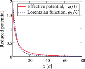
Figure 8: (Color online) The Thomas–Fermi potential (35) fitted by the Lorentzian function (37). Here, $q_{\textrm{TF}}a=0.1$, $U=\lambda/(2\pi\varepsilon_{0}\varepsilon_{\textrm{r}})$, and the fitting parameters are $A=1.544$, $B=0.780$, $C=0.046$.

Appendix B: Self-consistent calculations of the conductivity for a single charged line

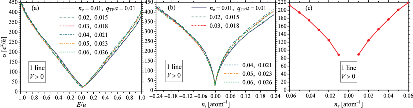
Figure 9: (Color online) Conductivity vs. the energy (a) and electron density (b), (c) for nonself-consistent (a), (b) and self-consistent (c) effective potentials $V\sim U=\lambda/(2\pi\varepsilon_{0}\varepsilon_{\textrm{r}})\in[0,\triangle]$ ($\triangle=0.25u$) describing a single charged line. Curve in (c) is plotted combining corresponding values for $\sigma$ on curves in (b). The correspondence between $q_{\textrm{TF}}$ used in calculations of the potential and respective $n_{e}$ is indicated in (a) and (b).

The Thomas–Fermi wavevector $q_{\textrm{TF}}$ entering the effective scattering potential [Eq. (2) or (35)] depends on the electron density $n_{e}$. In this appendix we check how this dependence affects the behavior of $\sigma$ as compared with the results obtained in Sec. II for a fixed $q_{\textrm{TF}}$; accounting for the density dependence makes our effective potential ‘self-consistent’.

We perform our calculations as follows. In the Kubo method used in this study it is not possible to change the scattering potential while changing the energy (or density) of the electrons. We therefore perform independent calculations for six different values of $q_{\textrm{TF}}$ obtaining six different dependencies $\sigma=\sigma(E)$ and $\sigma=\sigma(n_{e})$ as shown in Fig. 9(a) and Fig. 9(b), respectively. In each dependence $\sigma=\sigma(n_{e})$ we choose only one particular point (for both n- and p-types of charge carriers) where the electron density $n_{e}$ corresponds to $q_{\textrm{TF}}$ used in the calculation of this dependence (recall that $q_{\textrm{TF}}$ scales as $q_{\textrm{TF}}\propto\sqrt{|n_{e}|}$). Combining these six points on a single plot yields a ‘self-consistent’ curve $\sigma=\sigma(n_{e})$ as shown in Fig. 9(c). Figure 9 clear demonstrates that energy and electron density dependencies of conductivity exhibit respectively linear and sublinear behaviors, which are the same as corresponding behaviors of the conductivities for the case of a fixed $q_{\textrm{TF}}$, see Fig. 4. Note that electron–hole asymmetry in Fig. 9 is weak since the source of disorder here is due to a single line only (c.f., with 10 and 50 lines in Fig. 4).

Appendix C: Scattering amplitudes in the second Born approximation

The scattering problem $(\hat{H}_{0}+\hat{V}-E)\Psi_{\mathbf{k}}=0$, where $H_{0}$ denotes the free Hamiltonian and $\hat{V}$ a potential, has the formal solution

$$\Psi_{\mathbf{k}}=\phi_{\mathbf{k}}+\hat{G}_{0}\hat{V}\Psi_{\mathbf{k}}\,,$$ (38)

where $\phi_{\mathbf{k}}$ solves the free Schrödinger equation $(\hat{H}_{0}-E)\phi_{\mathbf{k}}=0$ and describes the state of the incident particles. The resolvent is given by $\hat{G}_{0}(z)=1/(z-\hat{H}_{0})$, where $z$ includes an infinitesimally small imaginary part.

In the context of the present work, $H_{0}$ stands for the Hamiltonian of pristine graphene in the single Dirac cone approximation, and $\hat{V}$ refers to the potential of a charged 1D defect (Appendix A). Although the form of $\hat{V}$ remains unspecified in what follows it is assumed to be a scalar in both sublattice and spin spaces. The spinor $\phi_{\mathbf{k}}(\mathbf{r})\equiv\langle\mathbf{r}|\phi_{\mathbf{k}}\rangle$ has the formCastro Netto review ; Peres_review ; DasSarma_review

$$\phi_{\mathbf{k}}(\mathbf{r})=u_{\mathbf{k}}e^{i\mathbf{k}\cdot\mathbf{r}}\,,$$ (39)

with

$$u_{\mathbf{k}}=\frac{1}{\sqrt{2}}\left(\begin{array}[]{c}1\\ se^{i\theta_{\mathbf{k}}}\end{array}\right)\,.$$ (40)

In the above, $\theta_{\mathbf{k}}\equiv\arctan(k_{y}/k_{x})$ and $s\equiv\textrm{sign}\left(E\right)$. Switching Eq. (38) to the position representation, we obtain the Lippmann–Schwinger equation

$$\Psi_{\mathbf{k}}(\mathbf{r})=\phi_{\mathbf{k}}(\mathbf{r})+\int d^{2}\mathbf{r}^{\prime}G_{0}(\mathbf{r}-\mathbf{r}^{\prime})V(\mathbf{r}^{\prime})\Psi_{\mathbf{k}}(\mathbf{r^{\prime}})\,,$$ (41)

where $G_{0}(\mathbf{r}-\mathbf{r}^{\prime})=\langle\mathbf{r}|\hat{G}_{0}(z)|\mathbf{r}^{\prime}\rangle$ is the Green function of the problem. The graphene Hamiltonian reads

$$\hat{H}_{0}=\hbar v_{F}\boldsymbol{\sigma}\cdot\hat{\mathbf{p}}\,,$$ (42)

and the Fourier transform of the Green function $G_{0}(\mathbf{p})=\int d^{2}\mathbf{r}\exp\left(-i\mathbf{p}\cdot\mathbf{r}\right)G_{0}(\mathbf{r})$ is given by

$$G_{0}(\mathbf{p})=\left(z-\hbar v_{F}\boldsymbol{\sigma}\cdot\mathbf{p}\right)^{-1}\,.$$ (43)

In what follows, unless stated otherwise, we set $\hbar\equiv 1\equiv v_{F}$ . It is also convenient to recast Eq. (43) in the form

$$G_{0}(\mathbf{p}) = g(\mathbf{p})(z+\boldsymbol{\sigma}\cdot\mathbf{p})\,,$$ (44)

$$g(\mathbf{p}) = \left(z^{2}-p^{2}\right)^{-1}.$$ (45)

where $z=E+is0^{+}$; the inclusion of a small imaginary part $is0^{+}$ amounts to consider outgoing waves (see below). For simplicity we focus on scattering of positive energy carriers (electrons), $s=1$. We write $E=k$ and evaluate the Green function in real space representation

$$G_{0}(\mathbf{r}-\mathbf{r}^{\prime}) =\left(E-i\boldsymbol{\sigma}\cdot\mathbf{\nabla}\right)\int\frac{d^{2}\mathbf{p}}{\left(2\pi\right)^{2}}e^{i\mathbf{p}\cdot(\mathbf{r}-\mathbf{r}^{\prime})}g(\mathbf{p})$$ (46)

$$=-\frac{i}{4}\left(k-i\boldsymbol{\sigma}\cdot\mathbf{\nabla}\right)H_{0}^{(1)}\left(k|\mathbf{r}-\mathbf{r}^{\prime}|\right)\,,$$ (47)

where $H_{n}^{(1)}\left(k|\mathbf{r}-\mathbf{r}^{\prime}|\right)$ is the first kind Hankel function of order $n$, whose asymptotic form is that of outgoing cylindrical waves. Using the property $\partial_{x}H_{0}^{(1)}(x)+H_{1}^{(1)}(x)=0$, the second term in Eq. (47) can be written in the simple form

$$\boldsymbol{\sigma}\cdot\mathbf{\nabla}H_{0}^{(1)}(k|\mathbf{r}-\mathbf{r}^{\prime}|)=-kH_{1}^{(1)}(k|\mathbf{r}-\mathbf{r}^{\prime}|)\sigma_{\theta}\,,$$ (48)

where we have introduced the matrix

$$\sigma_{\theta}\equiv\left(\begin{array}[]{cc}0&e^{-i\theta}\\ e^{i\theta}&0\end{array}\right)\,.$$ (49)

In the above, the angle $\theta\equiv\theta(\mathbf{r},\mathbf{r}^{\prime})$ is defined through the relation $\left(\mathbf{r}-\mathbf{r}^{\prime}\right)/|\mathbf{r}-\mathbf{r}^{\prime}|=\left(\cos\theta,\sin\theta\right)^{T}$.

Combining Eqs. (47)–(48) we obtain the explicit form of the Green function of pristine graphene

$$G_{0}(\mathbf{r}-\mathbf{r}^{\prime})=-\frac{ik}{4}\left[H_{0}^{(1)}(k|\mathbf{r}-\mathbf{r}^{\prime}|)+i\sigma_{\theta}H_{1}^{(1)}(k|\mathbf{r}-\mathbf{r}^{\prime}|)\right]\,.$$ (50)

The Lippmann–Schwinger equation now reads

$$\Psi_{\mathbf{\mathbf{k}}}(\mathbf{r}) = \phi_{\mathbf{\mathbf{k}}}(\mathbf{r})-\frac{ik}{4}\int d^{2}\mathbf{r}^{\prime}\left[H_{0}^{(1)}(k|\mathbf{r}-\mathbf{r}^{\prime}|)+\right.$$

$$\left.i\sigma_{\theta}H_{1}^{(1)}(k|\mathbf{r}-\mathbf{r}^{\prime}|)\right]V(\mathbf{r}^{\prime})\Psi_{\mathbf{k}}(\mathbf{r^{\prime}})\,.$$ (51)

To proceed, we assume that the main contribution to the scattering amplitude comes from evaluating the above integral within the region where $|\mathbf{r}-\mathbf{r}^{\prime}|\gg 1$. We note that although this procedure is accurate for short-range potentials, yielding the exact asymptotic form of the scattered wave function, it is otherwise an approximation.

The next step is to insert the asymptotic expressions for the Hankel functions

$$H_{0}^{(1)}(k|\mathbf{r}-\mathbf{r}^{\prime}|)\rightarrow\sqrt{\frac{2}{ik\pi|\mathbf{r}-\mathbf{\mathbf{r}^{\prime}}|}}e^{ik|\mathbf{r}-\mathbf{r}^{\prime}|}\,,$$ (52)

$$H_{1}^{(1)}(k|\mathbf{r}-\mathbf{r}^{\prime}|)\rightarrow-i\sqrt{\frac{2}{ik\pi|\mathbf{r}-\mathbf{\mathbf{r}^{\prime}}|}}e^{ik|\mathbf{r}-\mathbf{r}^{\prime}|},$$ (53)

into the Lippmann–Schwinger equation (51) to get

$$\Psi_{\mathbf{\mathbf{k}}}(\mathbf{r}) =\phi_{\mathbf{\mathbf{k}}}(\mathbf{r})-\sqrt{\frac{ik}{8\pi r}}e^{ikr}\int d^{2}\mathbf{r}^{\prime}e^{-i\mathbf{k^{\prime}}\cdot\mathbf{r}^{\prime}}\times$$

$$\left(1+\sigma_{\theta}\right)V(\mathbf{r}^{\prime})\Psi_{\mathbf{k}}(\mathbf{r^{\prime}}).$$ (54)

In the above, we have identified the wavevector at the point of observation, $k^{\prime}\equiv k\frac{\mathbf{r}}{r},$ and used $|\mathbf{r}-\mathbf{r}^{\prime}|\simeq\mathbf{r}-\mathbf{r}\cdot\mathbf{r}^{\prime}/r$ to simplify the argument of the exponentials in (52)–(53).

The first term in the Born series is obtained by replacing $\Psi_{\mathbf{k}}(\mathbf{r^{\prime}})\rightarrow\phi_{\mathbf{k}}(\mathbf{r^{\prime}})=e^{i\mathbf{k}\cdot\mathbf{r}^{\prime}}u_{\mathbf{k}}$ in the right-hand side of the Lippmann–Schwinger equation. In order to read out the scattering amplitude a few manipulations are still in order. Without loss of generality, setting $\theta_{\mathbf{k}}=0$, and identifying $\theta_{\mathbf{k}^{\prime}}$ with the scattering angle $\theta$, we find

$$\left(1+\sigma_{\theta}\right)u_{\mathbf{k}} = (1+e^{-i\theta})\frac{1}{\sqrt{2}}\left(\begin{array}[]{c}1\\ e^{i\theta}\end{array}\right)$$ (57)

$$\equiv \Xi(\theta)u_{\mathbf{k}^{\prime}},$$ (58)

where we have defined graphene’s Berry phase (form factor) term $\Xi(\theta)=1+e^{-i\theta}$. Substituting this result into Eq. (54) we arrive at the well-known FBA in two-dimensions

$$\Psi_{\mathbf{k}}(\mathbf{r})=\phi_{\mathbf{\mathbf{k}}}(\mathbf{r})+\frac{f_{\textrm{FBA}}(\theta)}{\sqrt{r}}e^{ikr}u_{\mathbf{k^{\prime}}}.$$ (59)

with

$$f_{\textrm{FBA}}(\theta)=-\frac{1}{v_{F}\hbar}\sqrt{\frac{ik}{8\pi}}\Xi(\theta)\tilde{V}(\mathbf{q}),$$ (60)

where $\mathbf{q}=\mathbf{k^{\prime}-}\mathbf{k}$ is the transferred wavevector and the relevant constants have been restored. We note that the above definition yields the usual form for the scattered current in two-dimensions, i.e.,

$$J(\theta)=\langle\tilde{\Psi}_{\mathbf{k}}(\mathbf{r})|\sigma_{\theta}|\tilde{\Psi}_{\mathbf{k}}(\mathbf{r})\rangle\propto\frac{|f_{\textrm{FBA}}(\theta)|^{2}}{r}\,,$$ (61)

with $\tilde{\Psi}_{\mathbf{k}}(\mathbf{r})\equiv\Psi_{\mathbf{k}}(\mathbf{r})-\phi_{\mathbf{\mathbf{k}}}(\mathbf{r})$ denoting the scattered component of the wave.

We move gears to the calculation of the second term in the Born series. The starting point is Eq. (41), which we iterate two times to get

$$\Psi_{\mathbf{k}}(\mathbf{r})=\phi_{\mathbf{k}}(\mathbf{r})+\int d^{2}\mathbf{r}^{\prime}\left[G_{0}(\mathbf{r}-\mathbf{r}^{\prime})V(\mathbf{r}^{\prime})\phi_{\mathbf{k}}(\mathbf{r^{\prime}})+\right.$$

$$\left.\int d^{2}\mathbf{r}^{\prime\prime}G_{0}(\mathbf{r}-\mathbf{r}^{\prime})V(\mathbf{r}^{\prime})G_{0}(\mathbf{r}^{\prime}-\mathbf{r}^{\prime\prime})V(\mathbf{r}^{\prime\prime})\phi_{\mathbf{k}}(\mathbf{r^{\prime\prime}})\right]\,.$$ (62)

We aim to simplify the second order contribution in the above expression [from now on referred to as $\Psi_{\mathbf{k}}^{(2)}(\mathbf{r})$]. As before, we replace $G_{0}(\mathbf{r}-\mathbf{r}^{\prime})$ by its asymptotic form

$$G_{0}(\mathbf{r}-\mathbf{r}^{\prime})\rightarrow-\sqrt{\frac{ik}{8\pi r}}e^{ikr}e^{-i\mathbf{k^{\prime}}\cdot\mathbf{r}^{\prime}}\tilde{\sigma}_{\theta},$$ (63)

with $\tilde{\sigma}_{\theta}\equiv 1+\sigma_{\theta}$, and insert it back into $\Psi_{\mathbf{k}}^{(2)}(\mathbf{r})$ as to obtain

$$\Psi_{\mathbf{k}}^{(2)}(\mathbf{r})=-\sqrt{\frac{ik}{8\pi r}}e^{ikr}\Upsilon_{\mathbf{k}\mathbf{k}^{\prime}}\,,$$ (64)

where

$$\Upsilon_{\mathbf{k}\mathbf{k}^{\prime}}=\int d^{2}\mathbf{r}^{\prime}d^{2}\mathbf{r}^{\prime\prime}e^{-i\mathbf{k^{\prime}}\cdot\mathbf{r}^{\prime}}\tilde{\sigma}_{\theta}V(\mathbf{r}^{\prime})G_{0}(\mathbf{r}^{\prime}-\mathbf{r}^{\prime\prime})V(\mathbf{r}^{\prime\prime})\phi_{\mathbf{k}}(\mathbf{r^{\prime\prime}})\,.$$ (65)

It is clear that $\tilde{\sigma}_{\theta}$ does not commute with the remaining terms in the integrand [remark that $G_{0}(\mathbf{r}^{\prime}-\mathbf{r}^{\prime\prime})$ contains a term proportional to $\sigma_{\alpha}$ with $\alpha\equiv\theta(\mathbf{r}^{\prime},\mathbf{r}^{\prime\prime})\neq\theta$; c.f., Eq.(50)], and hence we cannot directly identify the scattering amplitude as previously. Instead, we make use of Eq. (46) to write

$$\Upsilon_{\mathbf{k}\mathbf{k}^{\prime}}=\int\frac{d^{2}\mathbf{p}}{\left(2\pi\right)^{2}}g(\mathbf{p})\int d^{2}\mathbf{r}^{\prime\prime}V(\mathbf{r}^{\prime\prime})e^{-i(\mathbf{p}-\mathbf{k})\cdot\mathbf{r}^{\prime\prime}}\times$$

$$\left[\int d^{2}\mathbf{r}^{\prime}e^{-i\mathbf{k^{\prime}}\cdot\mathbf{r}^{\prime}}V(\mathbf{r}^{\prime})\tilde{\sigma}_{\theta}\left(k-i\sigma\cdot\boldsymbol{\nabla}^{\prime}\right)e^{i\mathbf{p}\cdot\mathbf{r}^{\prime}}\right]u_{\mathbf{k}}\,,$$ (66)

or, using the definition of Fourier transform,

$$\Upsilon_{\mathbf{k}\mathbf{k}^{\prime}}=\int\frac{d^{2}\mathbf{p}}{\left(2\pi\right)^{2}}\tilde{V}(\mathbf{p}-\mathbf{k})\left[\tilde{\sigma}_{\theta}G_{0}(\mathbf{p})\right]\tilde{V}(\mathbf{k}^{\prime}-\mathbf{p})u_{\mathbf{k}}\,.$$ (67)

In order to identify the scattering amplitude in the second Born approximation (SBA) we compute the contribution of $\Psi_{\mathbf{k}}^{(2)}(\mathbf{r})$ to the scattering flux. Neglecting terms of fourth order in the scattering potential, we find

$$J_{\textrm{SBA}}(\theta)=\langle\tilde{\Psi}_{\mathbf{k}}(\mathbf{r})|\sigma_{\theta}|\tilde{\Psi}_{\mathbf{k}}(\mathbf{r})\rangle=J(\theta)+\delta J(\theta)\,,$$

with $J(\theta)$ given by Eq. (61) and

$$\delta J(\theta)=-\frac{f_{\textrm{FBA}}^{*}(\theta)}{r}\sqrt{\frac{ik}{8\pi}}\langle u_{\mathbf{k^{\prime}}}|\sigma_{\theta}|\Upsilon_{\mathbf{k}\mathbf{k}^{\prime}}\rangle+\mathcal{\textrm{c.c.}}\>.$$ (68)

Using

$$\sqrt{2}\tilde{\sigma}_{\theta}\left(k+\sigma\cdot\mathbf{p}\right)u_{\mathbf{k}}=\left(\begin{array}[]{c}\Xi(\theta)k+pe^{-i\phi_{\mathbf{p}}}+pe^{i(\phi_{\mathbf{p}}-\theta)}\\ \Xi(-\theta)k+pe^{i\phi_{\mathbf{p}}}+pe^{i(\theta-\phi_{\mathbf{p}})}\end{array}\right)\,,$$ (71)

where $\phi_{\mathbf{p}}=\arctan(p_{y}/p_{x})$, we arrive at the following result

$$\langle u_{\mathbf{k^{\prime}}}|\sigma_{\theta}|\Upsilon_{\mathbf{k}\mathbf{k}^{\prime}}\rangle =\int\frac{d^{2}\mathbf{p}}{\left(2\pi\right)^{2}}\tilde{V}(\mathbf{p}-\mathbf{k})\left[k+pe^{-i\phi}+\right.$$

$$\left.+pe^{i(\phi-\theta)}+ke^{-i\theta}\right]\tilde{V}(\mathbf{k}^{\prime}-\mathbf{p})\,.$$ (72)

By the definition of scattered current $J_{\textrm{SBA}}(\theta)$, the SBA scattering amplitude is readily seen to be

$$f_{\textrm{SBA}}(\theta) =\sqrt{\frac{k}{8\pi}}\left\{\Xi(\theta)\tilde{V}(\mathbf{k}^{\prime}-\mathbf{k})+\right.$$

$$\int\frac{d^{2}\mathbf{p}}{\left(2\pi\right)^{2}}\tilde{V}(\mathbf{k}^{\prime}-\mathbf{p})\left[\Xi(\theta)\left(k+p\cos\phi_{\mathbf{p}}\right)+\right.$$

$$\left.\left.\bar{\Xi}(\theta)ip\sin\phi_{\mathbf{p}}g(\mathbf{p})\right]\tilde{V}(\mathbf{p}-\mathbf{k})\right\}\,,$$ (73)

where we defined $\bar{\Xi}(\theta)=\Xi(\theta+\pi)$ and dropped an innocuous phase factor $-\sqrt{i}$. We now specialize to potentials with inversion symmetry; these potentials have $\tilde{V}(\mathbf{q})=\tilde{V}(\mathbf{q})^{*}$ and therefore we can drop the imaginary term in last line of Eq. (73), which is odd under the transformation $\theta\rightarrow-\theta$, and hence does not contribute to transport cross sections. We thus arrive at our desired result

$$f_{\textrm{SBA}}(\theta) =\Xi(\theta)\sqrt{\frac{k}{8\pi}}\left\{\tilde{V}(\mathbf{k}^{\prime}-\mathbf{k})+\int\frac{d^{2}\mathbf{p}}{\left(2\pi\right)^{2}}\times\right.$$ (74)

$$\left.\tilde{V}(\mathbf{k}^{\prime}-\mathbf{p})\left(k+p\cos\phi_{\mathbf{p}}\right)g(\mathbf{p})\tilde{V}(\mathbf{p}-\mathbf{k})\right\}\,,$$

or, in a more compact form,

$$f_{\textrm{SBA}}(\theta) = \frac{\Xi(\theta)}{v_{F}\hbar}\sqrt{\frac{k}{8\pi}}\left[\tilde{V}(\mathbf{k}^{\prime}-\mathbf{k})+\int\frac{d^{2}\mathbf{p}}{\left(2\pi\right)^{2}}\times\right.$$ (75)

$$\left.\tilde{V}(\mathbf{k}^{\prime}-\mathbf{p})\langle u_{\mathbf{k}}|G_{0}(\mathbf{p})|u_{\mathbf{k}}\rangle\tilde{V}(\mathbf{p}-\mathbf{k})\right],$$

where $\hbar$ and $v_{F}$ have been restored.

Appendix D: Calculation of second Born amplitude for a charged line

In this appendix we evaluate the SBA transport cross section for a charged line with potential given by Eq. (16). We perform an analytical calculation of the $\mathcal{I}_{1}$ contribution [Eq. (12)] and evaluate the remaining contribution [Eq. (13)] numerically. The term $\mathcal{I}_{1}$ requires to evaluate the following integral

$$\eta_{1} =\int\frac{d^{2}\mathbf{p}}{\left(2\pi\right)^{2}}\frac{1}{k^{2}-\mathbf{p}^{2}+i0^{+}}$$

$$\qquad\frac{1}{q_{\mathtt{TF}}+|p_{x}-k_{x}|}\frac{1}{q_{\mathtt{TF}}+|k_{x}^{\prime}-p_{x}|},$$ (76)

which we do by first performing the integration over $k_{y}$ to get

$$\eta_{1} = \int\frac{dp_{x}}{2\pi}\frac{i}{2p_{0}}\frac{1}{q_{\mathtt{TF}}+|p_{x}-k_{x}|}\frac{1}{q_{\mathtt{TF}}+|k_{x}^{\prime}-p_{x}|}\,,$$ (77)

where $p_{0}=\sqrt{k^{2}-p_{x}^{2}}+i0^{+}$. To proceed, we divide the integration range into four subintervals: $p_{x}\geq k_{x}$, $k_{x}>p_{x}\geq k_{x}^{\prime}$, $k_{x}^{\prime}>p_{x}\geq-k_{x}$ and $p_{x}<-k_{x}$. Each of these contributions has a solution in terms of simple functions. We give the explicit solution for the real part of $\eta_{1}$. Since $p_{0}$ becomes pure imaginary for $|p_{x}|\geq k$, we have

$$\textrm{Re}\,\eta_{1} =\frac{1}{2}\left\{\int_{-\infty}^{-k}\frac{dp_{x}}{2\pi}\frac{1}{\sqrt{p_{x}^{2}-k^{2}}}\times\right.$$

$$\qquad\frac{1}{q_{\mathtt{TF}}-p_{x}+k_{x}}\frac{1}{q_{\mathtt{TF}}+k_{x}^{\prime}-p_{x}}+$$

$$\qquad\int_{k}^{\infty}\frac{dp_{x}}{2\pi}\frac{1}{\sqrt{p_{x}^{2}-k^{2}}}\times$$

$$\left.\qquad\frac{1}{q_{\mathtt{TF}}+p_{x}-k_{x}}\frac{1}{q_{\mathtt{TF}}-k_{x}^{\prime}+p_{x}}\right\}.$$ (78)

Without loss of generality we set $k_{x}=k$, $k_{x}^{\prime}=k\cos\theta$. The integral above then acquires the form

$$\textrm{Re}\,\eta_{1}=\frac{1}{32\pi\alpha_{\textrm{g}}}\frac{\chi(\theta)}{k_{F}^{2}\left(1-\cos\theta\right)},$$ (79)

with $k=k_{F}$ and

$$\chi(\theta) =\frac{-2\arccos\left(1+4\alpha_{\textrm{g}}\right)}{i\sqrt{1+\frac{1}{2\alpha_{\textrm{g}}}}}+\frac{\pi+2\arcsin\left(1-4\alpha_{\textrm{g}}\right)}{\sqrt{-1+\frac{1}{2\alpha_{\textrm{g}}}}}-$$

$$\frac{8\alpha_{\textrm{g}}\arccos\left(4\alpha_{\textrm{g}}-\cos\theta\right)}{\sqrt{1-\left(4\alpha_{\textrm{g}}-\cos\theta\right)^{2}}}+\frac{8\alpha_{\textrm{g}}\textrm{arccosh}\left(4\alpha_{\textrm{g}}+\cos\theta\right)}{\sqrt{\left(4\alpha_{\textrm{g}}+\cos\theta\right)^{2}-1}}\,,$$ (80)

and where used $q_{\mathtt{TF}}=4\alpha_{\textrm{g}}k_{F}$. The remaining term to be computed reads

$$\eta_{2} =\int\frac{d^{2}\mathbf{p}}{\left(2\pi\right)^{2}}\frac{p_{x}}{k^{2}-\mathbf{p}^{2}+i0^{+}}$$

$$\qquad\frac{1}{q_{\mathtt{TF}}+|k_{x}^{\prime}-p_{x}|}\frac{1}{q_{\mathtt{TF}}+|q_{x}-k_{x}|}\,.$$ (81)

The explicit form of $\eta_{2}$ is rather cumbersome and thus will not be given. The differential cross section is

$$\sigma(\theta)=|f_{1}(\theta)+f_{2}(\theta)|^{2}\,,$$ (82)

where $f_{1(2)}$ denotes the first (second) order contribution to the SBA amplitude [see Eq. (75)]. Defining $h_{1(2)}(\theta)\equiv f_{1(2)}(\theta)/\Xi(\theta)$, we obtain

$$\sigma(\theta)=|\Xi(\theta)|^{2}\left\{h_{1}(\theta)^{2}+2\textrm{Re}\left[h_{2}(\theta)\right]h_{1}(\theta)+\mathcal{O}(\Delta^{4})\right\},$$ (83)

and where we have used the fact that $h_{1}(\theta)\in\mathbb{R}$ for potentials with inversion symmetry. The first term yields the FBA transport cross section

$$\sigma_{\textrm{tp}}^{(\textrm{FBA})} = \int_{0}^{2\pi}d\theta\left(1-\cos\theta\right)|f_{1}(\theta)|^{2}$$ (84)

$$= \frac{k_{F}}{8\pi}\left(\frac{L\Delta}{\hbar v_{F}}\right)^{2}\int_{0}^{2\pi}d\theta\frac{\left(1-\cos\theta\right)|\Xi(\theta)|^{2}}{\left[2k_{F}\sin^{2}(\theta/2)+q_{\mathtt{TF}}\right]^{2}}$$

$$= \left(\frac{L\Delta}{\hbar v_{F}}\right)^{2}\frac{Q_{1}(\alpha)}{k_{F}},$$

with

$$Q_{1}(\alpha_{\textrm{g}})\equiv\frac{1}{8\pi}\int_{0}^{2\pi}d\theta\frac{\left(1-\cos\theta\right)|\Xi(\theta)|^{2}}{\left[2\sin^{2}(\theta/2)+4\alpha_{\textrm{g}}\right]^{2}}\,.$$ (85)

Remark that the transport relaxation rate is related to $\sigma_{\textrm{tp}}$ according to $\tau=(n_{l}v_{F}\sigma_{\textrm{tp}})^{-1}\sim k_{F}$, and therefore we conclude that the dc-conductivity

$$\sigma=\frac{2e^{2}}{h}v_{F}k_{F}\tau(k_{F})=\frac{2e^{2}}{h}\frac{k_{F}}{n_{l}\sigma_{\textrm{tp}}(k_{F})}\,,$$ (86)

is a quadratic (linear) function of the Fermi wavevector (electronic density). The latter property is preserved at all orders in perturbation theory as noted in Sec. III.

The second term in Eq. (83) yields the main correction to the FBA transport cross section; explicitly,

$$\delta\sigma_{\textrm{tp}}= \frac{k_{F}}{8\pi}\left(\frac{L\Delta}{\hbar v_{F}}\right)^{3}2k_{F}\int_{0}^{2\pi}d\theta\left(1-\cos\theta\right)\times$$

$$\qquad|\Xi(\theta)|^{2}\frac{\textrm{Re}\left[\eta_{1}(\theta)+\eta_{2}(\theta)\right]}{2k_{F}\sin^{2}(\theta/2)+q_{\mathtt{TF}}}\,.$$ (87)

Simplifying one obtains

$$\delta\sigma_{\textrm{tp}}=\left(\frac{L\Delta}{\hbar v_{F}}\right)^{3}\frac{Q_{2}(\alpha_{\textrm{g}})}{k_{F}}\,,$$ (88)

with

$$Q_{2}(\alpha_{\textrm{g}})\equiv\frac{1}{8\pi}\int_{0}^{2\pi}d\theta\frac{\left(1-\cos\theta\right)|\Xi(\theta)|^{2}}{2\sin^{2}(\theta/2)+4\alpha_{\textrm{g}}}\psi_{\textrm{SBA}}(\theta)\,,$$ (89)

and $\psi_{\textrm{SBA}}(\theta)\equiv 2k_{F}^{2}\textrm{Re}\left[\eta_{1}(\theta)+\eta_{2}(\theta)\right]$ is just a function of $\theta$ and $\alpha_{\textrm{g}}$ [recall that $\eta_{1(2)}$ varies as $k_{F}^{-2}$; see Eq. (79)]. Finally, one obtains for the SBA transport cross section

$$\sigma_{\textrm{tp}}^{(\textrm{SBA})} = \sum_{n=2,3}\left(\frac{L\Delta}{\hbar v_{F}}\right)^{n}\frac{Q_{n-1}(\alpha_{\textrm{g}})}{k_{F}}+\mathcal{O}(\Delta^{4}).$$ (90)

Collecting these results one obtains the following relation between the SBA and the FBA conductivities

$$\frac{\sigma_{\textrm{dc}}^{(\textrm{SBA})}}{\sigma_{\textrm{dc}}^{(\textrm{FBA})}}=\frac{\sigma_{\textrm{tp}}^{(\textrm{FBA})}}{\sigma_{\textrm{tp}}^{(\textrm{SBA})}}=1-\frac{L\Delta}{\hbar v_{F}}\frac{Q_{2}(\alpha_{\textrm{g}})}{Q_{1}(\alpha_{\textrm{g}})}+\mathcal{O}\left(\frac{L\Delta}{\hbar v_{F}}\right)^{2}.$$ (91)

The above result shows that for $\Delta>0$ ($\Delta<0$) the SBA decreases (increases) the dc conductivity with respect to the FBA result. Although only valid in the weak scattering regime, this dependence of the dc conductivity on the carrier polarity is in qualitatively agreement with the numerical results of Sec. II.

References

- (1) K. S. Novoselov, A. K. Geim, S. V. Morozov, D. Jiang, Y. Zhang, S. V. Dubonos, I. V. Grigorieva, and A. A. Firsov, Science 306, 666 (2004).
- (2) M. I. Katsnelson, Mater. Today 10, 20 (2007).
- (3) A. H. Castro Neto, F. Guinea, N. M. R. Peres, K. S. Novoselov, and A. K. Geim, Rev. Mod. Phys. 81, 109 (2009).
- (4) A. K. Geim and K. S. Novoselov, Nat. Mat. 6, 183 (2007).
- (5) W. A. de Heer, C. Berger, X. Wu, P. N. First, E. H. Conrad, X. Li, T. Li, M. Sprinkle, J. Hass, M. L. Sadowski, M. Potemski, and G. Martinez, Solid State Comm. 143, 92 (2007).
- (6) K. S. Kim, Y. Zhao, H. Jang, S. Y. Lee, J. M. Kim, K. S. Kim, J. H. Ahn, P. Kim, J. Y. Choi, and B. H. Hong, Nature 457, 706 (2009).
- (7) S. Bae, H. Kim, Y. Lee, X. Xu, J. -S. Park, Y. Zheng, J. Balakrishnan, T. Lei, H. R. Kim, Y. I. Song, Y. -J. Kim, K. S. Kim, B. Ozyilmaz, J. -H. Ahn, B. H. Hong, and S. Iijima, Nat. Nanotechnol. 5, 574 (2010).
- (8) A. Ferreira, X. Xu, C.-L. Tan, S.-K. Bae, N. M. R. Peres, B.-H. Hong, B. Ozyilmaz, and A. H. Castro Neto, EPL, 94, 28003 (2011).
- (9) F. Banhart, J. Kotakovski, and A. Krasheninnikov, ACS Nano 5, 26 (2011).
- (10) B. W. Jeong, J. Ihm, and G.-D. Lee, Phys. Rev. B 78, 165403 (2008).
- (11) O. V. Yazyev and S. G. Louie, Phys. Rev. B 81, 195420 (2010).
- (12) S. Malola, H. Hakkinen, and P. Koskinen, Phys. Rev. B 81, 165447 (2010).
- (13) H. S. Song, S. L. Li, H. Miyazaki, S. Sato, K. Hayashi, A. Yamada, N. Yokoyama, and K. Tsukagoshi, Sci. Rep. 2, 337 (2012).
- (14) X. Li, W. Cai, J. An, S. Kim, J. Nah, D. Yang, R. Piner, A. Velamakanni, I. Jung, E. Tutuc, S. K. Banerjee, L. Colombo, and R. S. Ruoff, Science, 324, 1312 (2009).
- (15) S. V. Morozov, K. S. Novoselov, M. I. Katsnelson, F. Schedin, D. C. Elias, J. A. Jaszczak, and A. K. Geim, Phys. Rev. Lett. 100, 016602 (2008).
- (16) X. Du, I. Skachko, A. Barker, and E. Y. Andrei, Nat. Nanotechnol. 3, 491 (2008).
- (17) K. I. Bolotin, K. J. Sikes, Z. Jiang, M. Klima, G. Fudenberg, J. Hone, P. Kim, and H. L. Stormer, Solis State Comm. 146, 351 (2008).
- (18) J. Lahiri, Y. Lin, P. Bozkurt, I. I. Oleynik, and M. Batzill, Nat. Nano. 5, 326 (2010).
- (19) J. Coraux, A. T. N’Diaye, C. Busse, and T. Michely, Nato Lett. 8, 565 (2008).
- (20) A. Hashimoto, K. Suenaga, A. Gloter, K. Urita, and S. Iijima, Nature 430, 870 (2004).
- (21) J. Červenka, M. I. Katsnelson, and C. F. J. Flipse, Nat. Phys. 5, 840 (2009).
- (22) D. Gunlycke and C. T. White, Phys. Rev. Lett. 106, 136806 (2011).
- (23) T. Okada, T. Kawai, and K. Nakada, J. Phys. Soc. Jpn. 80, 013709 (2011).
- (24) L. Kou, C. Tang, W. Guo, and C. Chen, ACS Nano 5, 1012 (2011).
- (25) M. Kindermann, Phys. Rev. Lett. 105, 216602 (2010).
- (26) A. R. Botello-Mendez, X. Declerck, M. Terrones, H. Terronesa, and J.-C. Charliera, Nanoscale 3, 2868 (2011).
- (27) J. Song, H. Liu, H. Jiang, Q.-f. Sun, and X. C. Xie, Phys. Rev. B 86, 085437 (2012).
- (28) S. S. Alexandre, A. D. Lúcio, A. H. Castro Neto, and R. W. Nunes, Nano Lett. 12, 5097 (2012).
- (29) O. V. Yazyev and S. G. Louie, Nat. Mater. 9, 806 (2010).
- (30) L. Jiang, G. Yu, W. Gao, Z. Liu, and Y. Zheng, Phys. Rev. B 86, 165433 (2012)
- (31) J. N. B. Rodrigues, N. M. R. Peres, and J. M. B. Lopes dos Santos, Phys. Rev. B 86, 214206 (2012).
- (32) D. V. Tuan, J. Kotakoski, T. Louvet, F. Ortmann, J. C. Meyer, and S. Roche, Nano Lett. 13, 1730 (2013).
- (33) J. W. Klos and I. V. Zozoulenko, Phys. Rev. B 82, 081414(R) (2010).
- (34) A. Ferreira, J. Viana-Gomes, J. Nilsson, E. R. Mucciolo, N. M. R. Peres, and A. H. Castro Neto, Phys. Rev. B 83, 165402 (2011).
- (35) H. Xu, T. Heinzel, and I. V. Zozoulenko, Phys. Rev. B 84, 115409 (2011).
- (36) T. M. Radchenko, A. A. Shylau, and I. V. Zozoulenko, Phys. Rev. B 86, 035418 (2012).
- (37) S. Roche, N. Leconte, F. Ortmann, A. Lherbier, D. Soriano, and J.-Ch. Charlier, Solid State Comm. 153, 1404 (2012).
- (38) S. Roche and D. Mayou, Phys. Rev. Lett. 79, 2518 (1997).
- (39) T. Markussen, R. Rurali, M. Brandbyge, and A.-P. Jauho, Phys. Rev. B 74, 245313 (2006); T. Markussen, Master thesis, Technical University of Denmark, 2006.
- (40) F. Triozon, J. Vidal, R. Mosseri, and D. Mayou, Phys. Rev. B 65, 220202(R) (2002).
- (41) F. Triozon, S. Roche, A. Rubio, and D. Mayou, Phys. Rev. B 69, 121410(R) (2004).
- (42) A. Lherbier, X. Blase, Y.-M. Niquet, F. Triozon, and S. Roche, Phys. Rev. Lett. 101, 036808 (2008).
- (43) A. Lherbier, B. Biel, Y.-M. Niquet, and S. Roche, Phys. Rev. Lett. 100, 036803 (2008).
- (44) A. Lherbier, Simon M.-M. Dubois, X. Declerck, S. Roche, Y.-M. Niquet, and J.-Ch. Charlier, Phys. Rev. Lett. 106, 046803 (2011).
- (45) S. Yuan, H. De Raedt, and M. I. Katsnelson, Phys. Rev. B 82, 115448 (2010).
- (46) N. Leconte, A. Lherbier, F. Varchon, P. Ordejon, S. Roche, and J.-C. Charlier, Phys. Rev. B 84, 235420 (2011).
- (47) A. Lherbier, Simon M.-M. Dubois, X. Declerck, Y.-M. Niquet, S. Roche, and J.-Ch. Charlier, Phys. Rev. B 86, 075402 (2012).
- (48) G. Trambly, de Laissardiere, and D. Mayou, Mod. Phys. Lett. B 25 1019 (2011).
- (49) H. Ishii, N. Kobayashi, and K. Hirose, Phys. Rev. B 82, 085435 (2010).
- (50) N. M. R. Peres, Rev. Mod. Phys. 82, 2673 (2010).
- (51) S. Das Sarma, S. Adam, E. H. Hwang, and E. Rossi, Rev. Mod. Phys. 83, 407 (2011).
- (52) O. Madelung, Introduction to Solid-State Theory (Springer, Berlin, 1996).
- (53) N. M. R. Peres, F. Guinea, and A. H. Castro Neto, Phys. Rev. B 73, 125411 (2006).
- (54) V. M. Pereira, F. Guinea, J. M. B. Lopes dos Santos, N. M. R. Peres, and A. H. Castro Neto, Phys. Rev. Lett. 96, 036801 (2006).
- (55) A. W. Tsen, L. Brown, M. P. Levendorf, F. Ghahari, P. Y. Huang, R. W. Havener, C. S. Ruiz-Vargas, D. A. Muller, Ph. Kim, and J. Park, Nature 467, 305 (2010).
- (56) C. H. Lewenkopf, E. R. Mucciolo, and A. H. Castro Neto, Phys. Rev. B 77, 081410(R) (2008).
- (57) J. P. Robinson, H. Schomerus, L. Oroszlany, and V. I. Fal’ko, Phys. Rev. Lett. 101, 196803 (2008).
- (58) T. O. Wehling, S. Yuan, A. I. Lichtenstein, A. K. Geim, and M. I. Katsnelson, Phys. Rev. Lett. 105, 056802 (2010).
- (59) J. M. Ziman, Principles of the Theory of Solids, 2nd ed. (Cambridge University Press, Cambridge, 1979).
- (60) The numerical evaluation of the Kubo formula in the weak scattering requires extremely large computational domains (needed to reach a diffusive transport) which is beyond our computational capabilities.
- (61) The potential energy in Fourier space considered here is obtained from a toy model of a finite line with , with being the electrostatic potential of an infinite line [Eq. (35)], and a smooth function of with the following properties: (1) is symmetric under reflection, and (2) varies slowly for and vanishes exponentially as , where . For instance, choosing , we obtain which upon substitution of and taking yields . We note that the same result can be obtained by broadening the delta function appearing in the potential of an infinite line.