ON THE AVERAGE NUMBER OF EDGES IN THETA GRAPHS

Theta graphs are important geometric graphs that have many applications, including wireless networking, motion planning, real-time animation, and minimum-spanning tree construction. We give closed form expressions for the average degree of theta graphs of a homogeneous Poisson point process over the plane. We then show that essentially the same bounds—with vanishing error terms—hold for theta graphs of finite sets of points that are uniformly distributed in a square. Finally, we show that the number of edges in a theta graph of points uniformly distributed in a square is concentrated around its expected value.

1 Introduction

Theta graphs [10, 16, 17] are important geometric graphs that have many applications, including wireless networking [2], motion planning [10], real-time animation [14], and minimum-spanning tree construction [24]. These graphs are defined on a planar point set, $S$, with an integer parameter $k$. For each $i\in\{1,\ldots,k\}$, define the cone

$$C_{i}=\{u\in\mathbb{R}^{2}:\measuredangle qou\in[2\pi(i-1)/k,2\pi i/k)\}\enspace,$$

where $q=(1,0)$ and $o=(0,0)$. In the $\theta_{k}$-graph, $\theta_{k}(S)$, each point $u\in S$ has an edge connecting it to the nearest point, if any, in the cone $C_{i}+u$, for each $i\in\{1,\ldots,k\}$. Here, “nearest” has a special meaning: The theta graph connects $u$ to the point whose orthogonal projection on the axis of $C_{i}+u$ is closest to $u$ (see Figure 1).

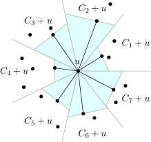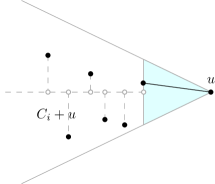(a)	(b)

Figure 1: A vertex, $u$, in a $\theta_{7}$-graph; (a) $u$ connects to the “nearest” point in each cone; (b) “nearest” is defined in terms of the projection onto the axis of each cone.

Theta graphs have two important properties that make them suited to a wide variety of applications: They are sparse; $\theta_{k}(S)$ has at most $k|S|$ edges and they are spanners; the length of the shortest path between any two vertices $u$ and $w$ is at most a constant (depending only on $k$ and not on $S$) times the Euclidean distance between $u$ and $w$. For any point set, $S$, $\theta_{k}(S)$ is a spanner for any $k\geq 4$ [5, 7, 8, 16, 23].

Note that, although $\theta_{k}(S)$ has at most $k|S|$ edges, it can also have significantly fewer edges. For example, if the points of $S$ all lie on a line, then $\theta_{k}(S)$ has only $|S|-1$ edges. More typical, though, is for $\theta_{k}(S)$ to have somewhere between $k|S|/2$ and $k|S|$ edges; each vertex $u\in S$ chooses $k$ edges of the graph but sometimes an edge $uw$ is chosen both by $u$ and $w$ and therefore it should not be counted twice.

1.1 The Models and Results

In this paper, we study the typical number of edges in $\theta_{k}$-graphs by studying the average number of edges in two different models of random point sets.

We begin, in Section 2, by studying (the infinite) $\theta_{k}$-graphs generated by a homogeneous Poisson point process with unit intensity over the entire Euclidean plane. In this model, we study the average degree of a vertex in the $\theta_{k}$-graph. For the $\theta_{k}$-graph, this quantity is at most $2k$ since each vertex defines $k$ edges of the graph and each edge has 2 endpoints. However, in some cases an edge $uw$ is mutual in the sense that the edge is created both by $u$ and by $w$. If we let $p_{k}$ denote the probability that an edge of the $\theta_{k}$-graph is mutual, then the average degree of the $\theta_{k}$ graph is

$$d_{k}=(2-p_{k})k\enspace.$$

(The second term corrects for the double-counting of mutual edges.) Thus, understanding the average degree of a $\theta_{k}$-graph boils down to computing $p_{k}$.

In Section 2.1 we show that, for all even integers $k\geq 4$,

$$p_{k}=\frac{\pi\sqrt{3}}{9}\approx 0.6045997883\enspace.$$

That is, the probability of an edge being mutual is independent of $k$. Thus, for all even integers $k\geq 4$, the average degree of a vertex is

$$d_{k}=\left(2-\frac{\pi\sqrt{3}}{9}\right)k\approx 1.395400212\cdot k\enspace.$$

In Section 2.2 we show that, for odd values of $k\geq 5$, the situation is very different. The mutual edge probability, $p_{k}$, depends on $k$ in a complicated way that includes trigonometric functions and square roots. However, the value of $p_{k}$ is significantly larger than $\frac{\pi\sqrt{3}}{9}$ for all odd values of $k$. Indeed, $p_{k}$ is a decreasing function of $k$ and

$$p_{k}\geq\lim_{k\to\infty}p_{k}=2\arctan(1/3)\approx 0.6435011088\enspace.$$

Thus, for all odd values of $k\geq 5$,

$$d_{k}\leq(2-2\arctan(1/3))k\approx 1.356498891k$$

Thus, in some sense, odd values of $k$ offer “more bang for the buck.”

In Section 3, we also study the i.u.d. model, in which a set, $S$, of $n$ points is independently and uniformly distributed in a square. In this model, we show that essentially the same bounds hold. Specifically, If $m_{k}$ is the number of edges of $\theta_{k}(S)$, then

$$\mathrm{E}[m_{k}]\in nd_{k}/2\pm O(k\sqrt{n\log n})\enspace\enspace,$$

where $d_{k}$, defined above, is the average degree of the $\theta_{k}$-graph in the Poisson model. We also give a concentration result that shows that the number of edges, $m_{k}$, is highly concentrated around its expected value. In particular

$$\Pr\{|m_{k}-nd_{k}/2|\geq k\sqrt{cn\log n}\}\leq n^{-\Omega(c)}\enspace.$$

1.2 Related Work

As discussed in the introduction, a plethora of literature exists on theta graphs and their applications, though most of this work focuses on worst-case analysis. One notable exception is the work of Devroye et al. [13] who study the maximum degree of theta graphs and show that, if $S$ is a set of $n$ points independently and uniformly distributed in a certain unit square, then $\theta_{k}(S)$ has maximum degree concentrated around $\Theta((\log n)/\log\log n)$.

In contrast, properties of other proximity graphs of random point sets have been studied extensively:

• Devroye [12] presents a general theorem for obtaining exact leading constants for the expected degree of a number of proximity graphs over point sets drawn from a large class of distributions. This theorem can be applied to Gabriel graphs, relative neighbourhood graphs, and nearest-neighbour graphs. This work [12, Section 7] also mentions “directional nearest-neighbour graphs,” now commonly known as Yao graphs [15, 24], and points out that the general theorem does not apply to these (nor does it apply to theta graphs—for the same reasons).

• Penrose and Yukich [21, 22] develop weak laws of large number and central limit theorems for several statistics of proximity graphs of random point sets under some assumptions about the locality of the graph and the statistic. Their results apply to statistics like total edge length and number of components of graphs such as $k$-nearest neighbour graphs, sphere of influence graphs, and Delaunay triangulations.

• Bern et al. [6] study the maximum degree of Delaunay triangulations of random point sets. Devroye et al. study the maximum degree of Gabriel graphs [13] of random point sets. Arkin et al. [3] study the length of the longest edge in Delaunay triangulations of random point sets.

• The issues of connectivity and giant components in the $r$-disk graph of random point sets—in which an edge $uw$ is present if and only if the distance between $u$ and $w$ is at most $r$—is the subject of intensive research and there are at least two books devoted to the topic [19, 20].

2 The Poisson Model

In the Poisson model, the number of points in any region with area is $A$ follows a Poisson distribution with parameter $A$. For definitions of point Poisson processes and distributions see, for example, Daley and Vere-Jones [11, Chapter 2]. For our purposes, the most important properties of the Poisson process are the following:

1. The probability that a particular Lebesgue-measurable set, $X$, whose area (Lebesgue measure) is $A$ is empty of points is exactly $e^{-A}$.

2. For disjoint regions $X_{1},\ldots,X_{v}$, the events “$X_{i}$ is empty of points”, for $i\in\{1,\ldots,v\}$ are independent.

Throughout this section, and in particular in Section 2.2, we have made extensive use of Mathematica to do symbolic integration and manipulation of trigonometric functions. Mathematica notebooks containing the code for these calculations are available at the first author’s webpage.

2.1 Analysis of $p_{k}$ for Even $k$

In this section we determine the value of $p_{k}$ for even values of $k$. Somewhat surprisingly, the value of $p_{k}$ in this case does not depend on $k$.

Lemma 1.

For even integers $k\geq 4$, $p_{k}=\frac{\pi\sqrt{3}}{9}\approx 0.6045997883$.

Proof.

Let $u$ be an arbitrary vertex in a $\theta_{k}$-graph and let $w$ be a vertex that $u$ has chosen as a neighbour in one of its cones, $C$ ($w$ is the “closest” vertex to $u$ in $C$). Let $T$ be the open isosceles triangle defined by $C$ and a line through $w$ that is orthogonal to the axis of $C$; refer to Figure 2. If the edge of $T$ opposite $u$ has length $\ell$, then $w$ partitions this edge into two pieces of length $r$ and $\ell-r$.

Figure 2: The edge $uw$ is mutual if and only if $T^{\prime}\setminus T$ is empty of points.

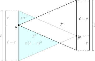
Let $T^{\prime}$ be the triangle obtained by reflecting $T$ through the midpoint of the edge $uw$ (so that $w$ is a vertex of $T^{\prime}$). Note that, because $k$ is even, $T^{\prime}$ coincides with one of $u$’s cones. In particular, if $w\in u+C_{i}$, then $T^{\prime}$ is contained in $w+C_{j}$ where $j=((i+k/2-1)\bmod k)+1$. Therefore, the edge $uw$ is mutual if and only if $T^{\prime}\setminus T$ contains no points. The area of $T^{\prime}\setminus T$ is

$$A(T^{\prime}\setminus T)=\alpha(r^{2}+(\ell-r)^{2})\enspace,$$

where $\alpha=\cos(\theta/2)/(4\sin(\theta/2))$. We now have enough information to compute the probability that the edge $uw$ is mutual conditional on $\ell$ and $r$:

$$\Pr\{\mbox{$uw$ is mutual}\mid\ell,r\}=\exp(-\alpha(r^{2}+(\ell-r)^{2}))\enspace.$$

Next, observe that the location of $w$ is uniformly distributed on the edge of $T$ opposite $u$, so the value of $r$ (conditioned on $\ell$) is uniform over $[0,\ell]$, unconditioning $r$ gives

$$f(\ell) \equiv\Pr\{\mbox{$uw$ is mutual}\mid\ell\}$$

$$=\int_{0}^{\ell}(1/\ell)\Pr\{\mbox{$uw$ is mutual}\mid\ell,r\}\,\mathrm{d}r$$

$$=\int_{0}^{\ell}(1/\ell)\exp(-\alpha(r^{2}+(\ell-r)^{2}))\,\mathrm{d}r$$

$$=\frac{\sqrt{\pi}}{\ell\sqrt{2\alpha}}\cdot\exp(-\alpha\ell^{2}/2)\cdot\operatorname{erf}(\ell\sqrt{\alpha/2})\enspace,$$

where

$$\operatorname{erf}(x)=\frac{2}{\sqrt{\pi}}\int_{0}^{x}e^{-z^{2}}\,\mathrm{d}z$$

is the Gauss error function [1, Section 7.2].

Next, we remove the conditioning on $\ell$. The triangle $T$ defines a region of area $\alpha\ell^{2}$ that is empty of points. Therefore, by Property 1 of the Poisson process, the cumulative distribution function of $\ell$ is given by

$$P(x)\equiv\Pr\{\ell\leq x\}=1-\exp(-\alpha x^{2})\enspace,$$

for $x\geq 0$. The probability density function of $\ell$ is therefore given by

$$p(x)\equiv\frac{d}{dx}P(x)=2\alpha x\cdot\exp(-\alpha x^{2})\enspace,$$

for $x\geq 0$. Finally, we obtain $p_{k}$ as

$$p_{k}=\int_{0}^{\infty}p(\ell)\cdot f(\ell)\,\mathrm{d}\ell=\frac{\pi\sqrt{3}}{9}\approx 0.6045997883\enspace.$$

2.2 Analysis of $p_{k}$ for Odd $k$

Next, we determine the values of $p_{k}$ for odd values of $k\geq 5$. Although the strategy for doing this is the same as the even case, the odd case turns out to be considerably more complicated; the value of $p_{k}$ does, indeed depend on $k$.

Lemma 2.

For odd $k\geq 5$,

$$p_{k}=2\left(\begin{array}[]{l}\arctan\left(2\left(\cos\left(\frac{\pi}{k}\right)+\cos\left(\frac{3\pi}{k}\right)\right)^{2}/(\alpha\beta)\right)\\ +\arctan\left(4\left(2\cos\left(\frac{2\pi}{k}\right)+\sin\left(\frac{2\pi}{k}\right)^{2}\right)/(\alpha\beta)\right)\end{array}\right)\cot\left(\frac{\pi}{k}\right)\beta/\left(\gamma\alpha\right)\enspace,$$

where

$$\gamma=4+11\cos\left(\frac{2\pi}{k}\right)+\cos\left(\frac{6\pi}{k}\right)\enspace,$$

$$\alpha=\sqrt{\frac{\left(27\cos\left(\frac{\pi}{k}\right)+17\cos\left(\frac{3\pi}{k}\right)+3\cos\left(\frac{5\pi}{k}\right)+\cos\left(\frac{7\pi}{k}\right)\right)\csc\left(\frac{\pi}{k}\right)}{\gamma}}\enspace,$$

and

$$\beta=\sqrt{\left(18\sin\left(\frac{2\pi}{k}\right)+18\sin\left(\frac{4\pi}{k}\right)+11\sin\left(\frac{6\pi}{k}\right)+\sin\left(\frac{8\pi}{k}\right)+\sin\left(\frac{10\pi}{k}\right)\right)}\enspace.$$

Proof.

The proof proceeds in the same manner as the proof of Lemma 1. Let $u$ be an arbitrary vertex in a $\theta_{k}$-graph and let $w$ be a vertex that $u$ has chosen as a neighbour in one of its cones, $C$. Let $T$ be the open isosceles triangle defined by $C$ and a line through $w$ that is orthogonal to the axis of $C$. See Figure 3. Assume that the side of $T$ opposite $u$ has length $2\ell$. Using a suitable rotation, we may assume that the axis of $C$ is horizontal and, by symmetry, we may assume that $w$ is on or above the axis of $C$.

Figure 3: The derivation of the $\Pr\{\mbox{$uw$ is mutual}\mid\ell,r\}$ for odd $k$.

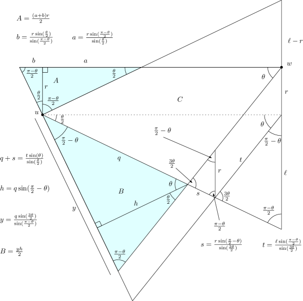
Under the preceding assumptions, $w$ is then uniformly distributed on a vertical segment of length $\ell$ whose endpoints are on the axis of $C$ and the upper boundary of $C$. Suppose that the distance from $w$ to the axis of $C$ is $r$. Then a straightforward, but tedious, calculation that mainly uses the law of sines shows that

$$\Pr\{\mbox{$uw$ is mutual}\mid\ell,r\}=\exp(-A-B)\enspace,$$

where

$$A=\frac{r^{2}}{\sin(2\pi/k)}$$

and

$$B=\frac{\cos(2\pi/k)}{2\sin(3\pi/k)\cos(\pi/k)}\cdot\left((\ell-r)\cos(2\pi/k)+\ell\right)^{2}$$

This calculation is illustrated in Figure 3 and the accompanying worksheet shows the simplifications that lead to the expressions for $A$ and $B$. Integrating over $r$ gives us

$$f(\ell)\equiv\Pr\{\mbox{$uw$ is mutual}\mid\ell\}=\int_{0}^{\ell}(1/\ell)\exp(-A-B)\,\mathrm{d}r.$$ (1)

Like the corresponding integral in the proof of Lemma 1, (1) has a closed-form that includes the Gauss error function.

In order to remove the conditioning on $\ell$, we need the probability density function for $\ell$. Proceeding as before, we have the cumulative distribution function

$$P(x)\equiv\Pr\{\ell\leq x\}=1-\exp(x^{2}/\tan(\pi/k))\enspace,$$

and the probability density function

$$p(x)\equiv\frac{d}{dx}P(x)=\left(\frac{2x}{\tan(\pi/k)}\right)\exp(x^{2}/\tan(\pi/k))$$

Finally, we determine $p_{k}$ by integrating over $\ell$:

$$p_{k}=\int_{0}^{\infty}p(\ell)\cdot f(\ell)\,\mathrm{d}{\ell}\enspace,$$

which (after introducing the variables $\alpha$, $\beta$, and $\gamma$) yields the expression for $p_{k}$ given in the statement of the lemma. ∎

3 Points in a Unit Square

Next we argue that results similar to Lemmas 1 and 2, albeit with lower-order error terms, hold for the graph $\theta_{k}(S)$, where $S$ is a set of $n$ points independently and uniformly distributed in the square $[0,\sqrt{n}]^{2}$ of area $n$. Observe that, in this model, the probability that any particular region $X\subseteq[0,\sqrt{n}]^{2}$ does not contain any points of $S$ is exactly $(1-A/n)^{n}=\exp(-A)-O(A/n)$, where $A$ is the area of $X$. This is consistent with the Poisson model up to an additive error of $O(1/n)$.

The primary work in this section involves finding quantities that look like those that appear in the previous section, but have an additive lower-order error term. To help manage these error terms, the notation $x=y\pm a$ denotes that $x$ is some value in the interval $[y-a,y+a]$. We will abuse this notation slightly by writing equations of the form $x\pm a=y\pm b$ when $[x-a,x+a]\subseteq[y-b,y+b]$. Occasionally, we may also integrate expressions that use this notation. In this case, we use the inequality $\int_{a}^{b}(x\pm c)\,\mathrm{d}x=\int_{a}^{b}x\pm c(b-a)$.

We sometimes encounter expressions like $A/(1-x)$, with $0<x<1/2$ which we bound by

$$A/(1-x)=A+O(Ax)\enspace.$$

We also frequently encouter expressions like $(1-A/n)^{n-c}$, where $c$ is a constant and $A<n/2$. We will always bound these as follows:

$$(1-A/n)^{n-c} =\frac{(1-A/n)^{n}}{(1-A/n)^{c}}$$

$$=\frac{\exp(-A)-O(A/n)}{(1-A/n)^{c}}$$

$$=\frac{\exp(-A)-O(A/n)}{\sum_{i=0}^{c}\binom{c}{i}(-A/n)^{i}}$$

$$=\frac{\exp(-A)-O(A/n)}{1-O(A/n)}$$

$$\geq\exp(-A)-O(A/n)$$

and, similarly,

$$(1-A/n)^{n-c} =\frac{(1-A/n)^{n}}{(1-A/n)^{c}}$$

$$\leq\frac{\exp(-A)}{(1-A/n)^{c}}$$

$$=\exp(-A)(1+O(A/n))\enspace.$$

3.1 Expected Number of Edges

In this section, we analyze the expected number of edges of $\theta_{k}(S)$. For each point $u\in S$ and each $i\in\{1,\ldots,k\}$, let $e(u,i)$ be the edge (if any) that $u$ chooses in its $i$th cone, $u+C_{i}$. That is, $e(u,i)$ is the edge $uw$ where $w\in u+C_{i}$ has the projection onto the axis of $u+C_{i}$ that is smallest among all points in $S\cap u+C_{i}$. We define the height of the edge $uw=e(u,i)$ as the distance between $u$ and the of the orthogonal projection of $w$ onto the axis of $u+C_{i}$.

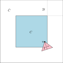
For our analysis, we partition $[0,\sqrt{n}]^{2}$ into a core, $C=[2t,\sqrt{n}-2t]^{2}$, where $t=\sqrt{ck\log n}$, and a near-boundary, $\bar{C}=[0,\sqrt{n}]^{2}\setminus C$ (see Figure 4). The motivation for partitioning into a core and near-boundary is that (1) there are not many points in the near-boundary and (2) points in the core behave almost exactly like points in the Poisson model. The following Lemma shows, for example, that points in the core nearly always have a neighbour in each of their cones.

Figure 4: The support, $[0,\sqrt{n}]^{2}$, is partitioned into a core, $C$, and a near-boundary $\bar{C}$. A point $u$ in the core almost surely has a neighbour in every cone, otherwise $u$ is incident on a large triangle, $T\subset[0,\sqrt{n}]^{2}$, that is empty of points.

Lemma 3.

For any $u\in S$ and any $i\in\{1,\ldots,k\}$, let $\mathcal{E}_{u,i}$ denote the event “$e(u,i)$ exists and has height at most $t$.” Then $\Pr\{\mathcal{E}_{u,i}\mid u\in C\}\geq 1-n^{-\Omega(c)}$.

Proof.

Fix some location of $u\in C$ and draw an open isosceles triangle, $T$, with apex $u$, contained in $u+C_{i}$, whose internal angle at $u$ is $\theta=2\pi/k$ and whose height is $t$ (see Figure 4). Observe that, since $u$ is in the core, $T\subset[0,\sqrt{n}]^{2}$. Furthermore, the area of $T$ is

$$A=t^{2}\tan(\pi/k)\in\Theta(t^{2}/k)=\Theta(c\log n)\enspace.$$

For $T$ to be empty of points in $S$, the $n-1$ points of $S\setminus\{u\}$ must all fall outside of $T$. Thus, we have

$$\Pr\{T\cap S=\emptyset\mid u\in C\} =(1-A/n)^{n-1}$$

$$\leq\exp(-A)(1+O(A/n))$$

$$\leq 2\exp(-A) n$$ (for sufficiently large )

$$=2\exp(-\Theta(c\log n))$$

$$=n^{-\Omega(c)}\enspace.$$

If $\mathcal{E}_{u,i}$ does not occur, this means that the event described above has occured. Therefore, $\Pr\{\mathcal{E}_{u,i}\mid u\in C\}\geq 1-n^{-\Omega(c)}$, as required. ∎

Our next lemma shows that edges generated by points in the core have essentially the same probability of being mutual as they do in the Poisson model.

Lemma 4.

For any $u\in S$ and any $i\in\{1,\ldots,k\}$, let $\mathcal{M}_{u,i}$ denote the event “$\mathcal{E}_{u,i}$ and $e(u,i)$ is mutual.” Then $\Pr\{\mathcal{M}_{u,i}\mid u\in C\}=p_{k}\pm O((\log n)^{2}/n)$.

Proof.

Throughout this proof, all probabilities we compute are conditional on $u\in C$, even when this is not explicitly stated. The proof is basically a reproving of Lemmas 1 and 2 that takes care to deal with boundary effects. Here, we will prove the case for even $k$ (Lemma 1) only. The case for odd $k$ (Lemma 2) can be done the same way.

We first compute the probability conditional on $\mathcal{E}_{u,i}$ and for fixed values of $\ell$ and $r$ as described in the proof of Lemma 1 and illustrated in Figure 2. The notations $\ell$, $r$, $T$, and $T^{\prime}$ all have the same meaning as in the proof of Lemma 1. The edge $e(u,i)$ is mutual if and only if the remaining $n-2$ points in $S\setminus\{u,w\}$—which are already conditioned on not being in $T$—also fall outside of $T^{\prime}$. The probability that this happens is

$$\Pr\{\mathcal{M}_{u,i}\mid\mathcal{E}_{u,i},\,\ell,\,r\} =\left(\frac{1-\operatorname{area}(T\cup T^{\prime})/n}{1-\operatorname{area}(T)/n}\right)^{n-2}$$

$$=\left(\frac{1-\operatorname{area}(T^{\prime}\setminus T)/n-\operatorname{area}(T)/n}{1-\operatorname{area}(T)/n}\right)^{n-2}$$

$$=\left(1-\frac{\operatorname{area}(T^{\prime}\setminus T)/n}{1-\operatorname{area}(T)/n}\right)^{n-2}$$

$$=\left(1-\frac{\alpha(r^{2}+(\ell-r)^{2})/n)}{1-\alpha\ell^{2}/n}\right)^{n-2}$$

$$=\left(1-\frac{\alpha(r^{2}+(\ell-r)^{2})(1+O(\alpha\ell^{2}/n))}{n}\right)^{n-2}$$

$$=\exp(-\alpha(r^{2}+(\ell-r)^{2})(1+O(\alpha\ell^{2}/n)))\pm O(\alpha\ell^{2}/n)$$

$$=\exp(-\alpha(r^{2}+(\ell-r)^{2}))\cdot\exp(O(\alpha^{2}\ell^{4}/n))\pm O(\alpha\ell^{2}/n)$$

$$=\exp(-\alpha(r^{2}+(\ell-r)^{2}))(1+O(\alpha^{2}\ell^{4}/n))\pm O(\alpha\ell^{2}/n)$$ (2)

$$=\exp(-\alpha(r^{2}+(\ell-r)^{2}))\pm O((\alpha^{2}\ell^{4}+\alpha\ell^{2})/n)$$

$$=\exp(-\alpha(r^{2}+(\ell-r)^{2}))\pm O((\alpha^{2}t^{4}+\alpha t^{2})/n)\enspace.$$

(Step (2) follows from the inequality $1+(e-1)x\geq e^{x}$ for $0\leq x\leq 1$.) We then remove the conditioning on $r$ by integrating:

$$f^{\prime}(\ell)\equiv \Pr\{\mathcal{M}_{u,i}\mid\mathcal{E}_{u,i},\,\ell\}$$

$$=\int_{0}^{\ell}(1/\ell)\left(\exp(-\alpha(r^{2}+(\ell-r)^{2}))\pm O((\alpha^{2}t^{4}+\alpha t^{2})/n)\right)\,\mathrm{d}r$$

$$=f(\ell)\pm O((\alpha^{2}t^{4}+\alpha t^{2})/n)\enspace,$$

where $f(\ell)$ is the same $f(\ell)$ defined in the proof of Lemma 1.

To finish, we need the distribution function for $\ell$ conditional on $\mathcal{E}_{u,i}$. The triangle $T$ has area $\alpha\ell^{2}$ so the probability that it is empty of points of $S\setminus\{u\}$ is $(1-\alpha\ell^{2}/n)^{n-1}$. Therefore, for $0\leq x\leq t$, we have the cumulative distribution function

$$P(x) \equiv\Pr\{\ell\leq x\mid\mathcal{E}_{u,i}\}$$

$$=\frac{\Pr\{\mathcal{E}_{u,i}\mbox{ and }\ell\leq x\}}{\Pr\{\mathcal{E}_{u,i}\}}$$

$$=\frac{\Pr\{\ell\leq x\}}{\Pr\{\mathcal{E}_{u,i}\}} 0\leq x\leq t \ell\leq x \mathcal{E}_{u,i}$$ (since , so implies )

$$=\frac{1-(1-\alpha x^{2}/n)^{n-1}}{1-(1-\alpha t^{2}/n)^{n-1}}$$

From this we obtain the density function

$$p^{\prime}(x) \equiv\frac{d}{dx}P(x)$$

$$=\frac{d}{dx}\frac{1-(1-\alpha x^{2}/n)^{n-1}}{1-(1-\alpha t^{2}/n)^{n-1}}$$

$$=\frac{2\alpha x(n-1)(1-\alpha x^{2}/n)^{n-2}}{n(1-(1-\alpha t^{2}/n)^{n-1})}$$

$$=\frac{2\alpha x(n-1)(\exp(-\alpha x^{2})\pm O(\alpha x^{2}/n))}{n(1-n^{-\Omega(c)})}$$

$$=\frac{2\alpha x(n-1)(\exp(-\alpha x^{2})\pm O(\alpha x^{2}/n))}{n-n^{-\Omega(c)}}$$

$$=\frac{2\alpha xn(\exp(-\alpha x^{2})\pm O(\alpha x^{2}/n))}{n-n^{-\Omega(c)}}(1-1/n)$$

$$=\frac{2\alpha x(\exp(-\alpha x^{2})\pm O(\alpha x^{2}/n))}{1-n^{-\Omega(c)}}(1-1/n)$$

$$=2\alpha x\left(\exp(-\alpha x^{2})\pm O(\alpha x^{2}/n)\right)(1+n^{-\Omega(c)})(1-1/n)$$

$$=2\alpha x\left(\exp(-\alpha x^{2})\pm O((1+\alpha x^{2})/n)\right)$$

$$=2\alpha x\exp(-\alpha x^{2})\pm O((\alpha x+\alpha^{2}x^{3})/n)$$

$$=2\alpha x\exp(-\alpha x^{2})\pm O((\alpha t+\alpha^{2}t^{3})/n)$$

$$=p(x)\pm O(\alpha^{2}t^{3}/n),$$

where $p(x)$ is the same $p(x)$ that appears in the proof of Lemma 1. And now we have enough information to finish:

$$\Pr\{\mathcal{M}_{u,i}\mid u\in C\} =\Pr\{\mathcal{E}_{u,i}\mid u\in C\}\cdot\Pr\{\mathcal{M}_{u,i}\mid\mathcal{E}_{u,i},\,u\in C\}$$

$$\qquad{}+\Pr\{\bar{\mathcal{E}}_{u,i}\mid u\in C\}\cdot\Pr\{\mathcal{M}_{u,i}\mid\bar{\mathcal{E}}_{u,i},\,u\in C\}$$

$$\geq\Pr\{\mathcal{E}_{u,i}\mid u\in C\}\cdot\Pr\{\mathcal{M}_{u,i}\mid\mathcal{E}_{u,i},\,u\in C\}$$

$$\geq\left(1-n^{-\Omega(c)}\right)\Pr\{\mathcal{M}_{u,i}\mid\mathcal{E}_{u,i},\,u\in C\}$$

$$=\left(1-n^{-\Omega(c)}\right)\int_{0}^{t}p^{\prime}(\ell)f^{\prime}(\ell)\,\mathrm{d}\ell$$

$$=\left(1-n^{-\Omega(c)}\right)\int_{0}^{t}(p(\ell)\pm O(\alpha^{2}t^{3}/n))\cdot(f(\ell)\pm O((\alpha^{2}t^{4}+\alpha t^{2})/n))\,\mathrm{d}{\ell}$$

$$=\left(1-n^{-\Omega(c)}\right)\int_{0}^{t}p(\ell)f(\ell)\pm O(p(\ell)(\alpha^{2}t^{4}+\alpha t^{2})/n+f(\ell)\alpha^{2}t^{3}/n+(\alpha^{5}t^{8}+\alpha^{3}t^{5})/n^{2})\,\mathrm{d}{\ell}$$

$$=\left(1-n^{-\Omega(c)}\right)\int_{0}^{t}p(\ell)f(\ell)\pm O((\alpha^{2}t^{4}+\alpha t^{2})/n+(\alpha^{5}t^{8}+\alpha^{3}t^{5})/n^{2})\,\mathrm{d}{\ell}$$

$$=\frac{\pi\sqrt{3}}{9}\pm O((\alpha^{2}t^{4}+\alpha t^{2})/n)$$

$$=\frac{\pi\sqrt{3}}{9}\pm O((\log n)^{2}/n)$$

and

$$\Pr\{\mathcal{M}_{u,i}\mid u\in C\} \leq\Pr\{\mathcal{E}_{u,i}\mid u\in C\}\cdot\Pr\{\mathcal{M}_{u,i}\mid\mathcal{E}_{u,i}\}+(1-\Pr\{\mathcal{E}_{u,i}\})$$

$$\leq\Pr\{\mathcal{E}_{u,i}\mid u\in C\}\cdot\Pr\{\mathcal{M}_{u,i}\mid\mathcal{E}_{u,i}\}+n^{-\Omega(c)}$$

$$=\frac{\pi\sqrt{3}}{9}\pm O((\log n)^{2}/n)\enspace.\qed$$

Lemma 5.

Let $S$ be a set of $n$ points independently and uniformly distributed in $[0,1]^{2}$. Then the expected number of edges of $\theta_{k}(S)$ is $nd_{k}/2\pm O(k\sqrt{nk\log n})$.

Proof.

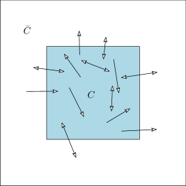
In this proof, it will be helpful to distinguish between directed and undirected edges. Undirected edges are the edges $\theta_{k}(S)$ that we have been considering throughout. In contrast, $uw=e(u,i)$ is a directed edge from $u$ to $w$. If $uw$ is mutual, then $wu=e(w,j)$ is a distinct directed edge from $w$ to $u$. In this way, if we let $E$ denote the number of undirected edges, $D$ the number of directed edges, and $M$ the number of mutual directed edges of $\theta_{k}(S)$. Then we have

$$E=D-M/2\enspace.$$

Let $E_{C}$, $D_{C}$, and $M_{C}$ denote the same quantities but only counting those edges with at least one endpoint in the core. (See Figure 5.)

Figure 5: The quantities $E_{C}$, $D_{C}$, and $M_{C}$: $E_{C}$ counts the number of segments, $D_{C}$ counts the number of arrowheads, and $M_{C}$ counts the number of segments with two arrowheads.

We begin with a lower bound:

$$\mathrm{E}[E] \geq\mathrm{E}[E_{C}]$$

$$=\mathrm{E}[D_{C}]-\mathrm{E}[M_{C}]/2$$

$$=\sum_{u\in S}\sum_{i=1}^{k}\Pr\{u\in C\}\left(\Pr\{\mathcal{E}_{u,i}\mid u\in C\}-\Pr\{\mathcal{M}_{u,i}\mid u\in C\}/2\right)$$

$$=k(\sqrt{n}-4t)^{2}\left(\Pr\{\mathcal{E}_{u,i}\mid u\in C\}-\Pr\{\mathcal{M}_{u,i}\mid u\in C\}/2\right)$$

$$\geq k(\sqrt{n}-4t)^{2}\left(1-n^{-\Omega(c)}-p_{k}/2-O((\log n)^{\frac{5}{2}}/n)\right)$$

$$\geq(kn-8t\sqrt{n})\left(1-n^{-\Omega(c)}-p_{k}/2-O((\log n)^{\frac{5}{2}}/n)\right)$$

$$=kn(1-p_{k}/2)-O(t\sqrt{n})$$

$$=nd_{k}/2-O(\sqrt{nk\log n})$$

For the upper-bound we proceed as follows:

$$\mathrm{E}[E] \leq\mathrm{E}[E_{C}]+\mathrm{E}[k\cdot|S\cap\bar{C}|]$$

$$=\mathrm{E}[E_{C}]+k(8t\sqrt{n}-16t^{2})$$

$$\leq\mathrm{E}[E_{C}]+4k\sqrt{nck\log n}$$

$$\leq nd_{k}/2+O((\log n)^{\frac{5}{2}})+4k\sqrt{nck\log n}$$

$$=nd_{k}/2+O(k\sqrt{nk\log n})$$

where the last step follows from a calculation similar to that done in the lower-bound. ∎

3.2 Concentration

Next, we show that the number of edges in this model is tightly concentrated about its expected value. We begin with the following result, which follows immediately from Hoeffding’s Inequality [9], and shows that the number of points in the core is highly concentrated around its expected value:

Lemma 6.

$\Pr\left\{\left||S\cap C|-(\sqrt{n}-4t)^{2}\right|\geq\sqrt{ck\log n}\right\}\in n^{-\Omega(c)}$.

To prove our concentration bound, we make use of a versatile concentration inequality due to McDiarmid [18, Lemma 1.2]:

Lemma 7 (McDiarmid’s Inequality).

Let $X_{1},\ldots,X_{n}$ be independent all taking values in the set $\mathcal{X}$ and let $f:\mathcal{X}^{n}\mapsto\mathbb{R}$ be a function such that

$$|f(x_{1},\ldots,x_{i},\ldots,x_{n})-f(x_{1},\ldots,x_{i}^{\prime},\ldots,x_{n})|\leq k\enspace,$$

for some $k>0$ and all $x_{1},\ldots,x_{n},x_{i}^{\prime}\in\mathcal{X}$ and all $i\in\{1,\ldots,n\}$. Then, for all $\epsilon>0$,

$$\Pr\left\{\left|f(X_{1},\ldots,X_{n})-\mathrm{E}[f(X_{1},\ldots,X_{n})]\right|\geq\epsilon\right\}\leq 2\exp(-2\epsilon^{2}/(nk^{2}))\enspace.$$

Lemma 8.

Let $S$ be a set of $n$ points independently and uniformly distributed in $[0,\sqrt{n}]^{2}$ and let $m_{k}$ denote the number of edges in $\theta_{k}(S)$. Then $\Pr\{|m_{k}-\mathrm{E}[m_{k}]|\geq k\sqrt{cn\log n}\}\leq n^{-\Omega(c)}$.

Proof.

Let $Q$ be a set of $k$ points chosen such that, for any point $u\in[0,\sqrt{n}]^{2}$, each of $u$’s $\theta_{k}$-cones contains exactly one point in $Q$. ($Q$ could be, for example, the vertices of a sufficiently large regular $k$-gon. See Figure 6.) We begin by studying $\theta_{k}(S\cup Q)$. This graph is somewhat more nicely behaved since each vertex in $S$ defines exactly $k$ directed edges.

Figure 6: The set $Q$ ensures that every vertex in $S$ has at least one point in each of its $\theta_{k}$-cones. This figure shows a possible set $Q$ for $k=5$.

For a set $S=\{u_{1},\ldots,u_{n}\}\subset[0,\sqrt{n}]^{2}$, let $f(u_{1},\ldots,u_{n})$ be the function that counts the number of edges in $\theta_{k}(S\cup Q)$. Observe that, for any $u_{1},\ldots,u_{n},u_{i}^{\prime}\in[0,1]^{2}$, we have that

$$|f(u_{1},\ldots,u_{i},\ldots,u_{n})-f(u_{1},\ldots,u_{i}^{\prime},\ldots,u_{n})|\leq k\enspace.$$

That is, moving $u_{i}$ to location $u_{i}^{\prime}$ can be though of as removing $u_{i}$, resulting in the loss of at most $k$ non-mutual edges emanating from $u_{i}$, followed by adding $u_{i}^{\prime}$ resulting in the creation of at most $k$ non-mutual edges emanating from $u_{i}^{\prime}$. Letting $m_{k}^{\prime}$ denote the number of edges in $\theta_{k}(S\cup Q)$, we immediately obtain, from McDiarmid’s Inequality,

$$\Pr\left\{\left|m_{k}^{\prime}-\mathrm{E}[m_{k}^{\prime}]\right|\geq k\sqrt{cn\log n}\right\}\leq 2\exp(-2c\log n)\in n^{-\Omega(c)}\enspace.$$

To extend this result to $m_{k}$, the number of edges of $\theta_{k}(S)$, we study $\Pr\{|m_{k}^{\prime}-m_{k}|\geq k\sqrt{cn\log n}\}$. If $|m_{k}^{\prime}-m_{k}|\geq k\sqrt{cn\log n}$ then the number of points of $S$ in the near-boundary $\bar{C}$ exceeds $\sqrt{cn\log n}$ or $\theta_{k}(S\cup Q)$ contains edges that join points in $Q$ to points in the core, $C$. Lemma 6 shows that the probability of the former event is at most $n^{-\Omega(c)}$, while Lemma 3 shows that the probability of the latter event is at most $n^{-\Omega(c)}$ ∎

4 Discussion

We have given exact closed-form expressions for the average degree of $\theta_{k}$-graphs for all $k\geq 4$. It is easily shown that $\theta_{k}$ graphs with $k=1,2,3$ are not spanners, so the cases $k\geq 4$ are the most important. We have also shown that the number of edges in a $\theta_{k}$-graph of $n$ points uniformly distributed in a square is highly concentrated around its expected value. These results can be used to inform practitioners about the optimal choice of $k$ to use in a particular application. Table 1 gives the numerical values of $d_{k}$, $p_{k}$, and $d_{k}/k$, for $k\in\{4,\ldots,20\}$.

$k$	$p_{k}$	$d_{k}$	$d_{k}/k$	$\hat{d}_{k}$
4	0.60459978	5.58160084	1.39540021	5.58190420
5	0.70168463	6.49157685	1.29831537	6.49280635
6	0.60459978	8.37240127	1.39540021	8.37587443
7	0.66778040	9.32553719	1.33221959	9.32743266
8	0.60459978	11.16320170	1.39540021	11.16338275
9	0.65740932	12.08331611	1.34259067	12.08319579
10	0.60459978	13.95400212	1.39540021	13.95657530
11	0.65259895	14.82141149	1.34740104	14.82372518
12	0.60459978	16.74480254	1.39540021	16.74624814
13	0.64993659	17.55082423	1.35006340	17.55520514
14	0.60459978	19.53560297	1.39540021	19.53693380
15	0.64830027	20.27549589	1.35169972	20.27565544
16	0.60459978	22.32640339	1.39540021	22.32956115
17	0.64722020	22.99725644	1.35277979	22.99979580
18	0.60459978	25.11720381	1.39540021	25.12062469
19	0.64646902	25.71708858	1.35353097	25.71956002
20	0.60459978	27.90800424	1.39540021	27.91343314

Table 1: Numeric values of $p_{k}$ and $d_{k}$.

Some of our results involved extensive symbolic manipulations that were done with the help of Mathematica. There is certainly the possibility of mistakes, either in the software or by its users. In order to help validate our analytical results, the final column in Table 1 also shows the results of the following experiment: 4,000 points were generated uniformly in the unit square $[0,1]^{2}$ and their $\theta_{k}$-graph was computed. The average degree of points in the square $[1/3,2/3]^{2}$ was then computed. The final column of Table 1 shows the average of these values taken over all 2,000 repetitions of this experiment. In all cases, it agrees with our theoretical results up to the first 3 digits.

Yao graphs [15, 24] are closely related to theta-graphs. In the Yao graph, $Y_{k}(S)$, each vertex $u$ is connected by an edge to the closest point in each of its theta cones, where closest is defined in terms of Euclidean distance. The same strategy we use to determine the average degree of $\theta_{k}(S)$ can be applied to $Y_{k}(S)$. Unfortunately, this fails to give closed form answers. In particular, when trying to repeat the proof of Lemma 1, we obtain the formula

$$p^{\prime}_{k}=\int_{0}^{\infty}\theta t\exp(-\theta t^{2}/2)\int_{0}^{t}\exp(-\theta t^{2}/2+t^{2}\sin(\gamma)\sin(\theta-\gamma)/\sin(\theta))\,\mathrm{d}\gamma\,\mathrm{d}t\enspace,$$

for which we are unable to obtain a closed form (here $\theta=2\pi/k$). Nevertheless, one can evaluate this integral numerically to obtain estimates of the mutual edge probability and average degree in Yao graphs.

References

- [1] M. Abramowitz and I. A. Stegun, editors. Handbook of Mathematical Functions. Dover Publications, New York, 9th edition, 1972.
- [2] K. M. Alzoubi, X.-Y. Li, Y. Wang, P.-J. Wan, and O. Frieder. Geometric spanners for wireless ad hoc networks. IEEE Trans. Parallel Distrib. Syst., 14(4):408–421, 2003.
- [3] E. M. Arkin, A. F. Anta, J. S. B. Mitchell, and M. A. Mosteiro. Probabilistic bounds on the length of a longest edge in delaunay graphs of random points in d-dimensions. In Proceedings of the 23rd Annual Canadian Conference on Computational Geometry (CCCG 2011), 2011.
- [4] D. Avis, B. Beresford-Smith, L. Devroye, H. A. ElGindy, E. Guévremont, F. Hurtado, and B. Zhu. Unoriented -maxima in the plane: Complexity and algorithms. SIAM Journal on Computing, 28(1):278–296, 1998.
- [5] L. Barba, P. Bose, J.-L. de Carufel, A. van Renssen, and S. Verdonschot. On the stretch factor of the theta-4 graph. arXiv:1303.5473, 2012.
- [6] M. Bern, D. Eppstein, and F. Yao. The expected extremes in a Delaunay triangulation. International Journal of Computational Geometry and Applications, 1:79–91, 1991.
- [7] N. Bonichon, C. Gavoille, N. Hanusse, and D. Ilcinkas. Connections between theta-graphs, delaunay triangulations, and orthogonal surfaces. In WG, volume 6410 of Lecture Notes in Computer Science, pages 266–278. Springer, 2010.
- [8] P. Bose, P. Morin, A. van Renssen, and S. Verdonschot. The theta-5 graph is a spanner. arXiv:1212.0570, 2012.
- [9] S. Boucheron, G. Lugosi, and O. Bousquet. Concentration inequalities. In Advanced Lectures on Machine Learning, volume 3176 of Lecture Notes in Computer Science, pages 208–240. Springer, 2004.
- [10] K. L. Clarkson. Approximation algorithms for shortest path motion planning (extended abstract). In A. V. Aho, editor, Proceedings of the 19th Annual ACM Symposium on Theory of Computing (STOC’87), pages 56–65. ACM, 1987.
- [11] D. J. Daley and D. Vere-Jones. An Introduction to the Theory of Point Processes. Volume I: Elementary Theory and Methods. Probability and Its Applications. Springer, 2003.
- [12] L. Devroye. The expected size of some graphs in computational geometry. Computers and Mathematics with Applications, 15:53–64, 1988.
- [13] L. Devroye, J. Gudmundsson, and P. Morin. On the expected maximum degree of Gabriel and Yao graphs. Advances in Applied Probability, 41(4):1123–1140, 2009.
- [14] M. Fischer, T. Lukovszki, and M. Ziegler. Geometric searching in walkthrough animations with weak spanners in real time. In G. Bilardi, G. F. Italiano, A. Pietracaprina, and G. Pucci, editors, Proceedings of the 6th Annual European Symposium on Algorithms (ESA’98), volume 1461 of Lecture Notes in Computer Science, pages 163–174. Springer, 1998.
- [15] B. E. Flinchbaugh and L. K. Jones. Strong connectivity in directional nearest-neighbor graphs. SIAM Journal on Algebraic Discrete Methods, 2(4), 1981.
- [16] J. M. Keil. Approximating the complete euclidean graph. In R. G. Karlsson and A. Lingas, editors, Proceedings of the 1st Scandinavian Workshop on Algorithm Theory (SWAT’88), volume 318 of Lecture Notes in Computer Science, pages 208–213, 1988.
- [17] J. M. Keil and C. A. Gutwin. Classes of graphs which approximate the complete euclidean graph. Discrete & Computational Geometry, 7:13–28, 1992.
- [18] C. McDiarmid. On the method of bounded differences. In J. Siemons, editor, Surveys in Combinatorics, volume 141 of London Mathematical Society Lecture Note Series, pages 148–188. Cambridge University Press, 1989.
- [19] R. Meester and R. Roy. Continuum percolation, volume 119 of Cambridge Tracts in Mathematics. Cambridge University Press, Cambridge, 1996.
- [20] M. Penrose. Random Geometric Graphs. Oxford University Press, 2003.
- [21] M. D. Penrose and J. E. Yukich. Central limit theorems for some graphs in computational geometry. The Annals of Applied Probability, 11(4):1005–1041, 2001.
- [22] M. D. Penrose and J. E. Yukich. Weak laws of large numbers in geometric probability. The Annals of Applied Probability, 13(1):277–303, 2003.
- [23] J. Ruppert and R. Seidel. Approximating the -dimensional complete Euclidean graph. In Proceedings of the 3rd Canadian Conference on Computational Geometry, pages 207–210, 1991.
- [24] A. C.-C. Yao. On constructing minimum spanning trees in k-dimensional spaces and related problems. SIAM Journal on Computing, 11(4):721–736, 1982.