Topological properties of a time-integrated activity driven network

Abstract

Here we consider the topological properties of the integrated networks emerging from the activity driven model [Perra at al. Sci. Rep. 2, 469 (2012)], a temporal network model recently proposed to explain the power-law degree distribution empirically observed in many real social networks. By means of a mapping to a hidden variables network model, we provide analytical expressions for the main topological properties of the integrated network, depending on the integration time and the distribution of activity potential characterizing the model. The expressions obtained, exacts in some cases, the results of controlled asymptotic expansions in others, are confirmed by means of extensive numerical simulations. Our analytical approach, which highlights the differences of the model with respect to the empirical observations made in real social networks, can be easily extended to deal with improved, more realistic modifications of the activity driven network paradigm.

I Introduction

Modern network science allows to represent and rationalize the properties and behavior of complex systems that can be represented in terms of a graph Newman (2010); Dorogovtsev (2010). Research in this area has focused in a twofold objective: A data-driven effort to characterize the topological properties of real networks Albert and Barabási (2002); Dorogovtsev and Mendes (2002); Caldarelli (2007), and a posterior modeling effort, aimed at understanding the microscopic mechanisms yielding the observed topological properties Albert and Barabási (2002); Newman (2010), as well as the effects that a complex topology has on dynamical processes running on top of it Dorogovtsev et al. (2008); Barrat et al. (2008).

Until recently, a large majority of work in the field of network science has been concerned with the study of static networks, i.e. networks in which topological properties do not change in time. Presently, however, a lot of attention is being devoted to the temporal dimension of networked systems Holme and Saramäki (2012). Indeed, many real networks are actually dynamical structures, in which edges appear, vanish or are rewired at different times scales. An important example is given by social networks Wasserman and Faust (1994), in which social relationships are represented by a succession of contact or communication events, continuously created or terminated between pairs of individuals. In this sense, the social networks previously considered in the literature Newman (2001); Barabási and Albert (1999); Liljeros et al. (2001) represent an projection or temporal integration of time-varying graphs, in which all the links that have appeared at least once in a time integration window $T$ are present in the projection.

The recent availability of large digital databases and the deployment of new experimental infrastructures have made possible the real-time tracking of social interactions in groups of individuals and the reconstruction of the corresponding temporal networks Oliveira and Barabasi (2005); Barabasi (2005); Gonzalez et al. (2008); Cattuto et al. (2010). The newly gathered empirical data poses new fundamental questions regarding the properties of temporal networks, questions which have been addressed through the formulation of theoretical models, aimed at explaining both the temporal patterns observed and their effects on the corresponding integrated networks Zhao et al. (2011); Jo et al. (2011); Song et al. (2010); Starnini et al. (2013).

Especially interesting in this perspective is the activity driven social network model recently introduced by Perra et al. Perra et al. (2012), aimed in particular to capture the relation between the dynamical properties of social temporal networks and the topological properties of their corresponding time projections. The key element in the definition of this model is the observation that the formation of social interactions is driven by the activity of individuals, urging them to interact with their peers, and by the empirical fact that different individuals show different levels of social activity Perra et al. (2012). Based in the concept of activity potential, defined as the probability per unit time that an individual engages in a social activity, Ref. Perra et al. (2012) proposed an activity driven social network model, in which individuals start interactions, that span for a fixed length of time $\Delta t$, with probability proportional to their activity potential. The model output is thus given by a sequence of graphs, depending on the distribution $F(a)$ of the activity potential, which are updated every time interval $\Delta t$. The topological properties of the integrated activity driven network were related in Ref. Perra et al. (2012) at the level of the degree distribution, which, by means of approximate arguments, was shown to be proportional to the activity potential distribution $F(a)$. However, despite the interest of the model, expressions for the rest of topological observables have been still lacking, a fact that hampers its possible validation as a generator of realistic integrated social networks, as well as the identification of the particular role that integration time has on the behavior of dynamical processes running on top of the temporal network Perra et al. (2012); Ribeiro et al. (2012).

Here we address the study of the aggregated network generated by the activity driven model, obtained by integrating the temporal network up to a given time $T$, by considering a mapping of the integrated network to a hidden variables model Boguñá and Pastor-Satorras (2003) depending on the activity potential distribution and the considered time $T$. We obtain a set of expressions for the degree distribution, degree-degree correlations and clustering coefficient of the aggregated network that are exact in the limit of large network size $N\to\infty$ and finite time $T$, and which are amenable to analytic asymptotic expansions in this same limit. The expressions obtained, confirmed by numerical simulations, corroborate the basic assumption of the activity driven model linking social activity with network topology. Moreover, the formalism proposed can be extended to generalizations of the activity driven model, opening thus the path to the analytical solution of model extensions, aimed at better reproducing the topological features of real integrated social networks.

We have organized the paper: Section III defines the activity driven network model. Sec. III gives a brief review of the hidden variables network formalism; Sec. IV deduces the mapping of the activity driven model onto this formalism. In Sec. V we compute the topological properties of the integrated activity network model as a function of time $T$, providing exact expressions as well as asymptotic results in the limit $T/N$ small, for different forms of the activity potential distribution. In Sec. VI we discuss the extension of the formalism presented to possible variations of the activity driven model. Finally, we summarize our results and conclusions in Sec. VII.

II The activity driven network model

The activity driven network model proposed in Ref. Perra et al. (2012) is defined in terms of $N$ individuals $i$ (agents), each one of them characterized by her activity potential $a_{i}$, defined as the probability that she engages in a social act/connection with other agents per unit time. The activity of the agents is a (quenched) random variable, extracted from the activity potential distribution $F(a)$, which can take a priori any form. The model is defined by means of a synchronous update scheme, time being measured in units of the life span of each connection $\Delta t$. It proceeds by creating a succession of instantaneous networks $\mathcal{G}_{t}$, $t=0,\Delta t,2\Delta t,\ldots,n\Delta t,\ldots$ At a given time $t$, all previous edges are deleted and we start with $N$ disconnected individuals. Each one of them is checked and becomes active with probability $a_{i}\Delta t$. Active agents generate $m$ links (start $m$ social interactions) that are connected to $m$ other agents selected uniformly at random. Finally, time is updated as $t\to t+\Delta t$. This procedure implies that all edges in the temporal network have the same constant time duration $\Delta t$. In order to avoid complications due to the differences in the number of emitted and received connections arising from using a synchronous approach, here we consider a probabilistic recipe for the instantaneous network construction: Each microscopic time step $\Delta t$, we choose $N$ agents, uniformly at random, and check sequentially each one of them for activation and eventual link emission. We avoid self and multiple connections.

To simplify the analytical calculations performed below, in the following we choose $\Delta t=m=1$. Both quantities can be however restored by a simple rescaling of the activity potential and the integration time $T$. We notice that imposing $\Delta t=1$ implies restricting the activity potential to be probability, and thus to be limited in the interval $a\in[0,1]$.

III Hidden variables formalism: A short review

The class of network models with hidden variables was introduced in Ref. Boguñá and Pastor-Satorras (2003) (see also Caldarelli et al. (2002); Söderberg (2002)) as a generalization of the random network Gilbert model Dorogovtsev (2010), in which the probability of connecting two vertices is not constant, but depends on some intrinsic properties of the respective vertices, their so-called hidden variables. This class of models is defined as follows: Starting from a set of $N$ disconnected vertices and a general hidden variable $h$, we construct an undirected network with no self-edges nor multiple connections, by applying these two rules:

1. To each vertex $i$, a variable $h_{i}$ is assigned, drawn at random from a probability distribution $\rho(h)$.

2. For each pair of vertices $i$ and $j$, $i\neq j$, with hidden variables $h_{i}$ and $h_{j}$, respectively, an edge is created with probability $r(h_{i},h_{j})$, the connection probability, which is a symmetric function bounded by $0\leq r(h,h^{\prime})\leq 1$.

Each model in the class is fully defined by the functions $\rho(h)$ and $r(h,h^{\prime})$, and all its topological properties can be derived as a function of these two parameters. These topological properties are encoded in the propagator $g(k|h)$, defined as the conditional probability that a vertex with hidden variable $h$ ends up connected to $k$ other vertices. The propagator is a normalized function, $\sum_{k}g(k|h)=1$, whose generating function $\hat{g}(z|h)=\sum_{k}z^{k}g(k|h)$ fulfills the general equation Boguñá and Pastor-Satorras (2003)

$$\ln\hat{g}(z|h)=N\sum_{h^{\prime}}\rho(h^{\prime})\ln\left[1-(1-z)r(h,h^{\prime})\right].$$ (1)

From this propagator, expressions for the topological properties of the model can be readily obtained Boguñá and Pastor-Satorras (2003):

• Degree distribution:

  $$P(k)=\sum_{h}g(k|h)\rho(h).$$ (2)

• Degree correlations, as measured by the average degree of the neighbors of the vertices of degree $k$, $\bar{k}^{nn}(k)$ Pastor-Satorras et al. (2001):

  $$\bar{k}^{nn}(k)=1+\frac{1}{P(k)}\sum_{h}\rho(h)g(k|h)\bar{k}^{nn}(h),$$ (3)

  where we have defined

  $$\bar{k}^{nn}(h)=\frac{N}{\bar{k}(h)}\sum_{h^{\prime}}\rho(h^{\prime})\bar{k}(h^{\prime})r(h,h^{\prime}),$$ (4)

  and

  $$\bar{k}(h)=N\sum_{h^{\prime}}\rho(h^{\prime})r(h,h^{\prime}),$$ (5)

  which is the average degree of the vertices with hidden variable $h$.

• Average clustering coefficient $\langle c\rangle$, defined as the probability that two vertices are connected, provided that they share a common neighbor Watts and Strogatz (1998)

  $$\langle c\rangle=\sum_{h}\rho(h)\bar{c}(h),$$ (6)

  where we have defined

  $$\bar{c}(h)=\sum_{h^{\prime},h^{\prime\prime}}p(h^{\prime}|h)r(h^{\prime},h^{\prime\prime})p(h^{\prime\prime}|h),$$ (7)

  and

  $$p(h^{\prime}|h)=\frac{N\rho(h^{\prime})r(h,h^{\prime})}{\bar{k}(h)}.$$ (8)

  Additionally, one can define the clustering spectrum, as measured by the average clustering coefficient of the vertices of degree $k$, $\bar{c}(k)$ Pastor-Satorras et al. (2001); Ravasz and Barabási (2003)

  $$\bar{c}(k)=\frac{1}{P(k)}\sum_{h}\rho(h)g(k|h)\bar{c}(h),$$ (9)

IV Mapping the integrated network to a hidden variables model

The activity driven network model generates a time series of instantaneous sparse networks, with an average degree $\langle k\rangle_{t}\simeq 2\langle a\rangle$, where $\langle a\rangle=\sum_{a}aF(a)$. The integrated network at time $T$ is constructed by performing the union of the instantaneous networks, i.e. $\mathcal{G}_{T}=\cup_{t=0}^{T}\mathcal{G}_{t}$. In this integrated network, vertices $i$ and $j$ will be joined by an edge if there has ever been a connection created between them in any of the instantaneous networks at $0\leq t\leq T$. The key point to map the integrated network to a hidden variables model resides in computing the probability $\Pi_{T}(i,j)$ that two vertices $i$ and $j$ become eventually joined at time $T$. This probability is given by $\Pi_{T}(i,j)=1-Q_{T}(i,j)$, where $Q_{T}(i,j)$, the probability that no connection has ever been created between agents $i$ and $j$ up to time $T$, can be calculated as follows: At time $T$, an agent $i$ will have become active $z$ times with probability $P_{T}(z)$. Given the definition of the model, at time $T$ we have selected $TN$ agents to check for activation. The number of times $z$ that agent $i$ has become active will be given by the binomial distribution

$$P_{T}(z)=\binom{TN}{z}\left(\frac{a_{i}}{N}\right)^{z}\left(1-\frac{a_{i}}{N}\right)^{TN-z},$$ (10)

and analogously for agent $j$. Now, vertices $i$ and $j$ will be connected in the integrated network if at least one of the links generated from $i$ reaches $j$, or vice-versa. Since every time that she becomes active, an agent creates a connection targeted to a randomly chosen peer, the probability $Q_{T}(i,j)$ is given by

$$Q_{T}(i,j) = \sum_{z_{i},z_{j}}P_{T}(z_{i})P_{T}(z_{i})\left(1-\frac{1}{N}\right)^{z_{i}}\left(1-\frac{1}{N}\right)^{z_{j}}$$ (11)

$$= \left[\left(1-\frac{a_{i}}{N^{2}}\right)\left(1-\frac{a_{j}}{N^{2}}\right)\right]^{TN},$$

where we have performed the summation using the probability distribution in Eq. (10). We see now that the probability that agents $i$ and $j$ are connected in the integrated network at time $T$ depends only on their respective activity potentials $a_{i}$ and $a_{j}$, which are random variables with distribution $F(a)$. The mapping to a hidden variables network is thus transparent:

• Hidden variable: $h\to a$.

• Distribution of hidden variables: $\rho(h)\to F(a)$.

• Connection probability: $r(h,h^{\prime})\to\Pi_{T}(a,a^{\prime})$.

At very large times, the integrated network emerging from the activity driven model will trivially tend to a fully connected network. Interesting topology will thus be restricted to the limit of small $T$ compared with the network size $N$. In this limit, Eq. (11) can be simplified, yielding

$$\Pi_{T}(a,a^{\prime}) = 1-Q_{T}(a,a^{\prime})\simeq 1-\left[1-\frac{(a+a^{\prime})}{N^{2}}\right]^{TN}$$ (12)

$$\simeq 1-\exp\left[-\lambda(a+a^{\prime})\right],$$

where we have neglected terms of order $\mathcal{O}(N^{-2})$ and defined the parameter

$$\lambda=\frac{T}{N}.$$ (13)

An explicit calculation of the connection probability for a factor $m>1$ and a time interval $\Delta t\neq 1$ can be easily performed; in the limit of large $N$ and constant $\lambda$, the only change ensuing is a rescaling of time, $T\to Tm$, the value of $\Delta t$ becoming canceled in the process of taking the limit $\lambda\to 0$.

V Topological properties of the integrated activity driven network

Here we will apply the formalism presented in Sec. III to provide analytic expressions characterizing the topology of the integrated network resulting from the activity driven model. For the sake of concreteness, we will focus in the following activity potential distributions, in the continuous $a$ limit:

• Constant activity:

  $$F(a)=\delta_{a,a_{0}},\;\;\mathrm{with}\;0<a_{0}<1.$$

• Homogeneous activity:

  $$F(a)=1/a_{\max},\;\;\mathrm{with}\;0\leq a\leq a_{\max}\leq 1.$$ (14)

• Power-law distributed activity:

  $$F(a)=(\gamma-1)\varepsilon^{\gamma-1}a^{-\gamma},\;\;\mathrm{with}\;a\in[\varepsilon,1].$$ (15)

In the last case, where we consider $\gamma>2$, in accordance with experimental evidence Perra et al. (2012), we have introduced a lower cut-off $0<\varepsilon\ll 1$ in order to avoid dangerous divergences in the vicinity of zero.

V.1 Degree distribution

In order to compute the degree distribution, we have to solve and invert the generating function equation Eq. (1), an almost impossible task to perform exactly, except in the case of very simple forms of the activity potential distribution. So, in the case of constant activity, $F(a)=\delta_{a,a_{0}}$, we have

$$\hat{g}(z|a_{0})=\left[z\Pi_{T}(a_{0},a_{0})+(1-\Pi_{T}(a_{0},a_{0}))\right]^{N},$$ (16)

which corresponds to the generating function of a binomial distribution Wilf (2006). Therefore, in the limit of large $N$ and constant $\lambda$, the degree distribution takes the Poisson form

$$P_{T}(k)=e^{-\mu}\frac{\mu^{k}}{k!}$$ (17)

with parameter $\mu=N\left(1-e^{-2\lambda a_{0}}\right)$, which, for fixed $T$ and large $N$, can be approximated as $\mu\simeq 2Ta_{0}$.

For a nontrivial activity distribution $F(a)$, we must resort to approximations. We therefore focus in the interesting limit of small $\lambda$, which corresponds to fixed $T$ and large $N$, which is the one yielding a non-trivial topology. In this limit, we can approximate the connection probability as

$$\Pi_{T}(a,a^{\prime})\simeq\lambda(a+a^{\prime}).$$ (18)

Introducing this expression into Eq. (1) and performing a new expansion at first order in $\lambda$, we obtain Boguñá and Pastor-Satorras (2003)

$$\ln\hat{g}(z|a) \simeq (1-z)\lambda N\sum_{a^{\prime}}F(a^{\prime})(a+a^{\prime})$$ (19)

$$= (1-z)\lambda N(a+\langle a\rangle).$$ (20)

The generating function of the propagator is a pure exponential, which indicates that the propagator itself is a Poisson distribution Wilf (2006), i.e.

$$g(k|a)=e^{-T(a+\langle a\rangle)}\frac{\left[T(a+\langle a\rangle)\right]^{k}}{\Gamma(k+1)},$$ (21)

where $\Gamma(x)$ is the Gamma (factorial) function Abramowitz and Stegun (1972). From Eq. (2) we obtain the general expression for the degree distribution

$$P_{T}(k)=\frac{T^{k}}{\Gamma(k+1)}\sum_{a}F(a)\left[a+\langle a\rangle\right]^{k}e^{-T(a+\langle a\rangle)}.$$ (22)

In the case of a homogeneous activity distribution, $F(a)={a_{\max}}^{-1}$, for which $\langle a\rangle=a_{\max}/2$, we can integrate directly Eq. (22), to obtain

$$P_{T}(k)=\frac{\Gamma\left(k+1,T\langle a\rangle\right)-\Gamma\left(k+1,3T\langle a\rangle\right)}{2T\langle a\rangle\;\Gamma(k+1)}.$$ (23)

where $\Gamma(x,z)$ is the incomplete Gamma function Abramowitz and Stegun (1972).

More complex forms of the activity distribution do not easily yield to an exact integration, and more approximations must be performed. In particular, the asymptotic form of the degree distribution can be obtained by performing a steepest descent approximation. Thus, we can write

$$P_{T}(k)=\frac{1}{\Gamma(k+1)}\int F(a)e^{\phi(a)}da,$$ (24)

where we have defined

$$\phi(a)=k\ln[T(a+\langle a\rangle)]-T(a+\langle a\rangle).$$ (25)

The function $\phi(a)$ has a sharp maximum around $a_{M}=\frac{k}{T}-\langle a\rangle$. Performing a Taylor expansion up to second order, we can write $\phi(a)\simeq\phi(a_{M})-\frac{T^{2}}{2k}\left[a-a_{M}\right]^{2}$, with $\phi(a_{M})=k\ln(k)-k$. Now, for $T^{2}/k\gg 1$, the function $e^{-\frac{T^{2}}{2k}\left[a-a_{M}\right]^{2}}$ is strongly peaked around the maximum $a_{M}$; therefore we can substitute the activity potential by its value at the maximum, to obtain

$$P_{T}(k) \simeq \frac{e^{\phi(a_{M})}F(a_{M})}{\Gamma(k+1)}\int_{-\infty}^{\infty}e^{-\frac{T^{2}}{2k}\left[a-a_{M}\right]^{2}}da$$ (26)

$$= \frac{\sqrt{2\pi k}k^{k}e^{-k}}{T\Gamma(k+1)}F\left(\frac{k}{T}-\langle a\rangle\right),$$

where we have extended the integration limits to plus and minus infinity. In the large $k$ limit, we can use Stirling’s approximation, $\Gamma(k+1)\sim\sqrt{2\pi k}k^{k}e^{-k}$, to obtain the asymptotic form

$$P_{T}(k)\sim\frac{1}{T}F\left(\frac{k}{T}-\langle a\rangle\right).$$ (27)

In this expression we recover, using more rigorous arguments, the asymptotic form of the integrated degree distribution obtained in Ref. Perra et al. (2012). The limits of validity of this expression are however now transparent, being explicitly $N\gg T\gg 1$ and $T^{2}\gg k\gg 1$.

For the case of constant activity, $F(a)=\delta_{a,a_{0}}$, the asymptotic form of the degree distribution is ${P_{T}(k)\sim\delta_{k,Ta_{0}}/T}$, while the exact form is a Poisson distribution centered at $2Ta_{0}$. For a uniform activity, on the other hand, the asymptotic prediction is a flat distribution, while the exact expression can be quite different, in particular for large and small values of $k$, see Eq. (23). For the case of a power-law distributed activity, in Fig. 1 we plot the degree distribution $P_{T}(k)$ of the aggregated network at different values of $T$ for networks of size $N=10^{6}$ and two different values of $\gamma$. As we can see, for such large networks sizes and values of $\lambda\sim 10^{-2}-10^{-3}$, the asymptotic expression Eq. (27) represents a very good approximation to the model behavior. In Fig. 2 we plot the degree distribution for a smaller network size $N=10^{3}$. As one can see, a numerical integration of Eq. (22) recovers exactly the behavior of $P_{T}(k)$ even for small values of $k$. With such small network size, however, the asymptotic prediction of Eq. (27) is less good, as shown in the inset of Fig. 2.

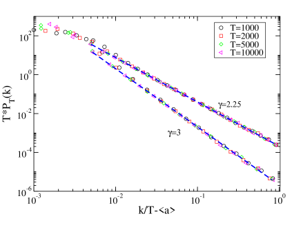
Figure 1: (color online) Rescaled degree distribution $P_{T}(k)$ for integrated networks corresponding to different values of $T$, with power law activity distribution with exponents $\gamma=3$ and $2.25$. Network size $N=10^{6}$. The behavior predicted by Eq. (27) is represented as dashed lines.

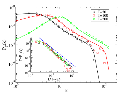
Figure 2: (color online) Degree distribution $P_{T}(k)$ for integrated networks corresponding to different values of $T$, with power law activity distribution with exponent $\gamma=2.25$. Network size $N=10^{3}$. The result of a numerical integration of Eq. (22) is showed as continuous lines. Inset: Rescaled $P_{T}(k)$ shown against Eq. (27), dashed in blue.

V.2 Degree correlations

We start from Eq. (5), which takes the form, as a function of time

$$\bar{k}_{T}(a)=N[1-e^{-\lambda a}\Psi(\lambda)],$$ (28)

where $\Psi(\lambda)$ is the Laplace transform

$$\Psi(\lambda)\equiv\sum_{a}F(a)e^{-\lambda a}.$$ (29)

We can now use Eq. (4), which leads to the exact expression

$$\bar{k}^{nn}_{T}(a)=N\left\{1-\Psi(\lambda)\frac{\Psi(\lambda)-\Psi(2\lambda)e^{-\lambda a}}{1-\Psi(\lambda)e^{-\lambda a}}\right\}.$$ (30)

In order to obtain an explicit expression for $\bar{k}^{nn}_{T}(k)$ we must perform the integral in Eq. (3). In the case of a constant activity potential, $F(a)=\delta_{a,a_{0}}$, we have $P_{T}(k)=g(k|a_{0})$. Since in this case $\Psi(\lambda)=e^{-\lambda a_{0}}$, we have

$$\bar{k}^{nn}_{T}(k)=1+N\left[1-e^{-2\lambda a_{0}}\right]\simeq 1+2Ta_{0},$$ (31)

where the last expression corresponds to the limit of small $\lambda$. This function is independent of $k$, indicating that the integrated network corresponding to constant activity potential has no degree correlations.

For more complex forms of $F(a)$, we resort to an expansion in powers of $\lambda$ to obtain an approximate expression, which at lowest order takes the form

$$\bar{k}^{nn}_{T}(a)\simeq\frac{\lambda N}{a+\langle a\rangle}\left[\langle a^{2}\rangle+\langle a\rangle^{2}+2a\langle a\rangle\right].$$ (32)

Inserting this expression into Eq. (3), and considering the Poisson form of the propagator Eq. (21), we can write

$$\bar{k}^{nn}_{T}(k) \simeq 1+\frac{T^{2}(\langle a^{2}\rangle+\langle a\rangle^{2})}{kP(k)}\int daF(a)g(k-1|a)+$$

$$\frac{2T^{2}\langle a\rangle}{kP(k)}\int daaF(a)g(k-1|a)$$

$$\simeq 1+T^{2}\frac{P(k-1)}{kP(k)}\left[\sigma_{a}^{2}+2\langle a\rangle\left(\frac{k}{T}\right)\right],$$

where in the last expression we have performed the steepest descent approximation used to obtain Eq. (26), and $\sigma_{a}^{2}=\langle a^{2}\rangle-\langle a\rangle^{2}$ is the variance of the activity potential $F(a)$. In the limit of large $k$, where $P(k-1)/P(k)\sim 1$, we have the general form for the degree correlations

$$\frac{\bar{k}^{nn}_{T}(k)-1}{T}\simeq 2\langle a\rangle+\sigma_{a}^{2}\left(\frac{k}{T}\right)^{-1}.$$ (33)

This expression recovers in a natural way the exact result for constant activity potential, where $\sigma_{a}^{2}=0$. From Eq. (33) we conclude that, in general, for an non-constant activity distribution, the integrated networks resulting from the activity driven model show disassortative mixing by degree Newman (2002), with a $\bar{k}^{nn}_{T}(k)$ function decreasing as a function of $k$. This disassortative behavior, which can be however quite mild in the case of small variance $\sigma_{a}$, as in the case of a power law distributed activity with small $\varepsilon$, is in any case at odds with the assortative form observed for degree correlations in real social networks Newman (2010).

In Fig. 3 we check the validity of Eq. (32) and the asymptotic form Eq. (33) in the case of power law distributed activity. We observe that the prediction of Eq. (32) recovers exactly the model behavior, also in the case of small activity $a$ (shown in the inset). The degree correlation, $\bar{k}^{nn}_{T}(k)$, is also correctly captured by the asymptotic form Eq. (33). Note however that, since the variance $\sigma_{a}$ is small (of order $\varepsilon^{\gamma-1}$ for $\gamma<3$ and order $\varepsilon^{2}$ for $\gamma>3$), the net change in the average degree of the neighbors is quite small, and the integrated network can be considered as approximately uncorrelated without incurring in a gross error.

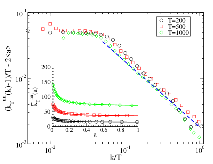
Figure 3: (color online) Main: Rescaled average degree of the nearest neighbors of the vertices of degree $k$, $\bar{k}^{nn}_{T}(k)$, for the integrated network with size $N=10^{4}$ and power law activity distribution with $\gamma=2.5$, for different values of $T$. The prediction of Eq. (33) is dashed in blue. Inset: Average degree of the neighbors of the vertices with activity $a$, $\bar{k}^{nn}_{T}(a)$, for the same integrated network. The predictions from Eq. (32) are shown as continuous lines.

V.3 Clustering coefficient

The expression of the clustering spectrum at time $T$, $\bar{c}_{T}(k)$, takes the form, from Eq. (9)

$$\bar{c}_{T}(k)=\frac{1}{P_{T}(k)}\sum_{a}F(a)g(k|a)\bar{c}_{T}(a).$$ (34)

Using Eqs. (7), (8) and the expression for $\bar{k}(a)$, we can write the exact form

$$\bar{c}_{T}(a)=1-\left[\frac{\Psi(\lambda)-e^{-\lambda a}\Psi(2\lambda)}{1-e^{-\lambda a}\Psi(\lambda)}\right]^{2}.$$ (35)

Again in the simplest case of a constant activity potential, $F(a)=\delta_{a,a_{0}}$, we have $\bar{c}_{T}(a)=1-e^{-2\lambda a_{0}}$, which leads to a clustering spectrum

$$\bar{c}_{T}(k)\equiv\langle c\rangle_{T}=1-e^{-2\lambda a_{0}}\simeq\frac{2Ta_{0}}{N},$$ (36)

where the last expression is valid for small $\lambda$. The clustering spectrum is in this case constant, and equal to the average clustering coefficient. For fixed time $T$, it is inversely proportional to the network size, in correspondence to a purely random network. It increases with $T$, saturating at $\langle c\rangle_{\infty}=1$ for a fully connected network in the infinite time limit.

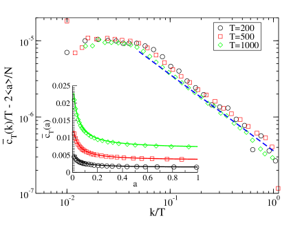
Figure 4: (color online) Main: Rescaled clustering coefficient of the nodes of degree $k$, $c_{T}(k)$, of the integrated network with size $N=10^{4}$ and power law activity distribution with $\gamma=2.5$, for different values of $T$. The prediction of Eq. (39) is dashed in blue. Inset: Clustering coefficient of the nodes with activity $a$, $c_{T}(a),$ of the same integrated network. The predictions from Eq. (37) are shown as continuous lines.

For a general activity potential distribution, we need to perform again an expansion in $\lambda$, which in this case takes the form, at first order in $\lambda$,

$$\bar{c}(a)\simeq\frac{2\lambda}{a+\langle a\rangle}[\langle a^{2}\rangle+a\langle a\rangle].$$ (37)

Inserting this form into Eq. (34), and performing the same steepest descend approximation applied in Eq. (V.2), we obtain

$$\bar{c}(k)\simeq\frac{2T^{2}}{N}\frac{P(k-1)}{kP(k)}\left[(\langle a^{2}\rangle-\langle a\rangle^{2})+\langle a\rangle\left(\frac{k}{T}\right)\right].$$ (38)

In the limit of large $k$, we obtain the general form of the clustering spectrum, valid for any activity potential,

$$\frac{\bar{c}(k)}{T}\simeq\frac{2\langle a\rangle}{N}+\frac{2\sigma_{a}^{2}}{N}\left(\frac{k}{T}\right)^{-1}.$$ (39)

In Fig. 4 we plot the clustering coefficient as a function of the degree (main) and the activity (inset), in the case of power law distributed activity. We observe that both Eq. (37) and Eq. (39) recover correctly the clustering coefficient behavior.

VI Model extensions

The potency of the hidden variables formalism we have introduced above to solve the activity driven model allows to easily extended it to tackle the analysis of generalized models inspired in the same principles. We can consider, indeed, different rules for activation and reception of connections. The only limitation to be imposed in order to properly implement the formalism is that connection rules must be local, i.e. involving only properties of the emitting and receiving agents. As a simple example, we consider a sort of “inverse” activity driven model, in which every agent $i$ becomes active with the same constant probability $a_{i}=a_{0}$ and, when active, she sends a connection to another agent $j$, chosen at random with probability proportional to some (quenched) random quantity $b_{j}$, the attractiveness of the node, i.e. with probability $b_{j}/\langle b\rangle N$. In this case, one can easily repeat the steps of the mapping presented in Sec. IV: The number of times $z$ that agent $i$ becomes active is now

$$P^{\prime}_{T}(z)=\binom{TN}{z}\left(\frac{a_{0}}{N}\right)^{z}\left(1-\frac{a_{0}}{N}\right)^{TN-z},$$ (40)

and the probability that $i$ and $j$ never become connected up to time $T$ is

$$Q^{\prime}_{T}(i,j) = \sum_{z_{i},z_{j}}P^{\prime}_{T}(z_{i})P^{\prime}_{T}(z_{j})\left(1-\frac{b_{j}}{\langle b\rangle N}\right)^{z_{i}}\left(1-\frac{b_{i}}{\langle b\rangle N}\right)^{z_{j}}$$

$$= \left[\left(1-\frac{a_{0}b_{i}}{\langle b\rangle N^{2}}\right)\left(1-\frac{a_{0}b_{j}}{\langle b\rangle N^{2}}\right)\right]^{TN}$$

$$\simeq \exp\left[-\lambda^{\prime}(b_{i}+b_{j})\right],$$

where we have defined the new parameter $\lambda^{\prime}=a_{0}T/\langle b\rangle N$ and, in the last step of the previous expressions, we have performed and expansion for large $N$ a finite $T$. From here, we obtain $\Pi^{\prime}_{T}(i,j)=1-Q^{\prime}_{T}(i,j)$. As we can see, this modified model is exactly mappable to the activity driven model (see Eq. (12), with the simple translation $\lambda\to\lambda^{\prime}$; all the general expression derived above hold thus in this case, and can be worked out, upon providing the appropriate expression for the attractiveness distribution $F(b)$.

VII Conclusions

The activity driven model represents an interesting approximation to temporal networks, providing an preliminary explanation of the origin of the degree distribution of integrated social networks, in terms of the heterogeneity of the agents’ activity, and the distribution of this quantity. Here we have explored the full relation between topology and activity distribution, obtaining analytical expressions for several topological properties of the integrated social networks for a general activity potential, in the thermodynamic limit of large number of agents, $N\rightarrow\infty$, and finite integration time $T$. To tackle this issue, we have applied the hidden variables formalism, by mapping the aggregated network to a model in which the probability of connecting two nodes depends on the hidden variable (in this case represented by the activity potential) of those nodes. Our analysis is complemented by numerical simulations in order to check theoretical predictions against concrete examples of activity potential distributions. Using our formalism, we can demonstrate rigorously that the integrated degree distribution at time $T$ takes the same functional form as the activity potential distribution, as a function of the rescaled degree $k/T-\langle a\rangle$. This is however an asymptotic result, which is well fulfilled for an activity potential power-law distributed, as empirically measured in a wide range of social interaction settings, which fails for simple constant or homogeneous distributions. We also show that the aggregated networks show in general disassortative degree correlations, at odds with the assortative mixing revealed in real social networks. The clustering coefficient is low, $\langle c\rangle\sim T/N$, comparable with a random network.

Our study opens interesting direction for future work, concerning, for example, the clarification of role of integration time in the properties of dynamical process on activity driven networks, and the possible modifications of the activity driven network model, in order to incorporate some properties of real social networks currently missed, such as a high clustering coefficient, assortative mixing by degree or a community structure Newman (2010).