On the $B^{*^{\prime}}\to B$ transition

Abstract

We present a first $N_{\rm f}=2$ lattice estimate of the hadronic coupling $g_{12}$ which parametrises the strong decay of a radially excited $B^{*}$ meson into the ground state $B$ meson at zero recoil. We work in the static limit of Heavy Quark Effective Theory (HQET) and solve a Generalised Eigenvalue Problem (GEVP), which is necessary for the extraction of excited state properties. After an extrapolation to the continuum limit and a check of the pion mass dependence, we obtain $g_{12}=-0.17(4)$.

I Introduction

Questions have been raised recently on the poor handling of excited states in the analyses of experimental data and their comparison with theoretical predictions, particularly in the case of heavy-light $B$ and $D$ mesons . For instance, it has been advocated that the $\sim$ 3$\sigma$ discrepancy observed between exclusive and inclusive estimates of the CKM matrix element $V_{cb}$ might be reduced if the transition $B\to D^{\prime}$ were large. This attractive hypothesis implies a suppression of the $B\to D^{(*)}$ hadronic form factors, as a study in the OPE formalism suggests GambinoRD . On the other hand, it has been argued that the light-cone sum rule determination of the $g_{D^{*}D\pi}$ coupling, which parametrises the $D^{*}\to D\pi$ decay, likely fails to reproduce the experimental measurement unless one explicitly includes the contribution from the first radial excited $D^{(*)^{\prime}}$ state on the hadronic side of the three-point Borel sum rule BecirevicVP . Comparison with sum rules is of particular importance because the heavy mass dependence of $\hat{g}_{Q}\equiv\frac{g_{H^{*}H\pi}f_{\pi}}{2\sqrt{m_{H}m_{H^{*}}}}$ deduced from recent lattice simulations OhkiPY ; BecirevicYB ; BulavaEJ ; DetmoldGE ; BecirevicPF ; BernardoniIP and experiment Godang:2013im seems much weaker than expected from analytical methods KhodjamirianHB , as shown in Figure 1.

$J^{P}$	ground state	radial excitation
$0^{-}$	$H$	$H^{{}^{\prime}}$
$1^{-}$	$H^{*}$	$H^{*^{\prime}}$
$0^{+}$	$H_{0}^{*}$	$H_{0}^{*^{\prime}}$
$1^{+}$	$H_{1}^{*}$	$H_{1}^{*^{\prime}}$

Table 1: Spectroscopy of the lowest states of heavy-light $H\equiv$ $B$ and $D$ mesons.

Techniques have been developed to study excited states of mesons using lattice QCD BulavaNP , especially to extract the spectrum BurchCC ; BlossierVZ ; MohlerKE ; MahbubRM . Similar techniques can now be applied to three-point correlation functions to perhaps illuminate the phenomenological issues discussed above. In this letter we will report on the lattice computation of $g_{12}\equiv\langle B^{*^{\prime}}|{\cal A}_{i}|B\rangle$ in the static limit of HQET, where ${\cal A}_{i}$ is the axial vector bilinear of light quarks and $B^{*^{\prime}}$ is polarised along the $i$th direction. As a by-product of our work, we will also report on the computation of $g_{11}\equiv\langle B^{*}|{\cal A}_{i}|B\rangle$ and $g_{22}\equiv\langle B^{*^{\prime}}|{\cal A}_{i}|B^{\prime}\rangle$.

The Heavy Quark Symmetry of leading order HQET is well suited for our qualitative study. As the spectra of excited $B$ and $B^{*}$ mesons are degenerate, it is enough to solve a single Generalized Eigenvalue Problem (GEVP) while degrees of freedom $\sim$ $m_{b}$, that are somehow irrelevant for the dynamics of the cloud of light quarks and gluons that governs the process we examine, are integrated out. The plan of the letter is the following: in Sec. II we describe our approach while in Sec. III we present our lattice set-up and discuss results before concluding in Sec. IV.

Figure 1: Experimental measurement Godang:2013im , lattice computations OhkiPY ; BecirevicYB ; BulavaEJ ; DetmoldGE ; BecirevicPF and sum rules estimates KhodjamirianHB of $\hat{g}_{c}$, $\hat{g}_{b}$ and $\hat{g}\equiv\hat{g}_{\infty}$. We have performed a weighted average of recent $\hat{g}$ lattice results at ${\rm N_{f}}=2$ with respect to the error quoted in OhkiPY ; BecirevicYB ; BulavaEJ ; DetmoldGE .

II Extraction of $\langle B^{*^{\prime}}|{\cal A}_{i}|B\rangle$

The transition amplitude of interest is parametrised by

$$\langle B^{*^{\prime}}(p^{\prime},\epsilon_{\lambda})|{\cal A}^{\mu}|B(p)\rangle = 2m_{B^{*^{\prime}}}A_{0}(q^{2})\frac{\epsilon^{(\lambda)}\cdot q}{q^{2}}q^{\mu}+(m_{B}+m_{B^{*^{\prime}}})A_{1}(q^{2})\left(\epsilon^{(\lambda)\,\mu}-\frac{\epsilon^{(\lambda)}\cdot q}{q^{2}}q^{\mu}\right)$$ (1)

$$+ A_{2}(q^{2})\frac{\epsilon^{(\lambda)}\cdot q}{m_{B}+m_{B^{*^{\prime}}}}\left[(p_{B}+p_{B^{*^{\prime}}})^{\mu}+\frac{m^{2}_{B}-m^{2}_{B^{*^{\prime}}}}{q^{2}}q^{\mu}\right]\,,$$

with $q=p^{\prime}-p$. In the zero recoil kinematic configuration where $\vec{p}=\vec{p}^{\prime}=\vec{0}$, one has $q^{2}_{\rm max}=(m_{B^{*^{\prime}}}-m_{B})^{2}$ so that

$$\langle B^{*^{\prime}}(p^{\prime},\epsilon_{\lambda})|{\cal A}^{i}|B(p)\rangle=(m_{B}+m_{B^{*^{\prime}}})A_{1}(q^{2}_{\rm max})\epsilon^{(\lambda)\,i}\,.$$ (2)

At that stage it is useful to introduce the HQET normalisation of states: $|H\rangle=\sqrt{2m_{H}}|H\rangle_{\rm HQET}$, with $\langle H(p)|H(p^{\prime})\rangle=2E(p)\delta^{3}(\vec{p}-\vec{p}^{\prime})$:

$$\langle B^{*^{\prime}}(p^{\prime},\epsilon_{\lambda})|{\cal A}^{i}|B(p)\rangle_{\rm HQET}=\frac{m_{B}+m_{B^{*^{\prime}}}}{2\sqrt{m_{B}m_{B^{*^{\prime}}}}}A_{1}(q_{\rm max}^{2})\epsilon^{(\lambda)\,i}\,.$$ (3)

In the static limit we are left with $\langle B^{*^{\prime}}(p^{\prime},\epsilon_{\lambda})|{\cal A}^{i}|B(p)\rangle_{\rm HQET}=A_{1}(q_{\rm max}^{2})\epsilon^{(\lambda)\,i}$. Choosing the quantization axis along the $z$ direction and the polarisation vector $\epsilon^{\mu}(0)=\left(\begin{array}[]{c}0\\ 0\\ 0\\ 1\\ \end{array}\right)$, with the metric (+,-,-,-), we get finally $A_{1}(q^{2}_{\rm max})=\langle B^{*^{\prime}}(p^{\prime},\epsilon_{0})|{\cal A}^{3}|B(p)\rangle_{\rm HQET}$. Of course, extracting $g_{11}\equiv\hat{g}$ and $g_{22}$ is similar, except that the relevant axial form factors are defined at $q^{2}=0$.

GEVP methods MichaelNE ; LuscherCK ; BlossierKD are a very efficient tool to study excited states on the lattice. We consider $N\times N$ matrices of two-point correlation functions together with the corresponding matrices of three-point correlation functions $C^{(^{\prime})(2)}_{ij}(t)\equiv\langle O^{(^{\prime})}_{i}(t)O^{(^{\prime}){\dagger}}_{j}(0)\rangle$ and $C^{(3)}_{ij}(t,t_{s})\equiv\langle O^{\prime}_{i}(t_{s})O_{\Gamma}(t)O^{\dagger}_{j}(0)\rangle$, where $i,j$ represent different wave functions and Dirac structures with quantum numbers generically denoted $(h)$. More explicitly, the $O_{i}$ are interpolating fields of pseudoscalar static-light mesons, the $O^{\prime}_{i}$ interpolating fields of vector static-light mesons and $O_{\Gamma}$ the axial vector light-light bilinear of quarks.

In HQET the spectral decomposition reads $C^{(^{\prime})(2)}_{ij}(t)=\sum_{n}\psi^{*(h^{(^{\prime})})}_{ni}\psi^{(h^{(^{\prime})})}_{nj}e^{-E_{n}t}$, $\psi^{(h^{(^{\prime})})}_{ni}=\langle M^{(h^{(^{\prime})})}_{n}|\hat{O}^{{\dagger}(^{\prime})}_{i}|0\rangle$. The purpose of solving GEVP is to construct quantities which tend toward the desired excited state properties asymptotically in time. In practice we solve

$$\sum_{j}C^{(2)}_{ij}(t)v^{(n)}_{j}(t,t_{0})=\sum_{j}\lambda^{(n)}(t,t_{0})C^{(2)}_{ij}(t_{0})v^{(n)}_{j}(t,t_{0}),\quad\lambda^{(n)}(t,t_{0})=e^{-E^{\rm eff}_{n}(t,t_{0})(t-t_{0})}\,.$$ (4)

We will use two ratio methods, GEVP and sGEVP, to extract the matrix element $M_{mn}\equiv\langle M^{(h)}_{n}|\hat{O}_{\Gamma}|M^{(h^{\prime})}_{m}\rangle$. Those ratios converge quickly as the contribution of higher excited states is strongly suppressed BulavaYZ and read:

$$R^{\rm GEVP}_{mn}(t,t_{s}) = \frac{\langle v^{(n)}(t_{s}-t,t_{0}),C^{(3)}_{\Gamma}(t,t_{s})v^{(m)}(t,t_{0})\rangle\lambda^{(m)}(t_{0}+a,t_{0})^{-t/2}\lambda^{(n)}(t_{0}+a,t_{0})^{t-t_{s}/2}}{\sqrt{\langle v^{(n)}(t_{s}-t,t_{0}),C^{(2)}(t_{s}-t)v^{(n)}(t_{s}-t,t_{0})\rangle\langle v^{(m)}(t,t_{0}),C^{\prime(2)}(t)v^{(m)}(t,t_{0})\rangle}}$$ (5)

$$\stackrel{{\scriptstyle t/a\gg 1,(t_{s}-t)/a\gg 1}}{{\sim}} M_{mn}+{\cal O}(e^{-\Delta_{N+1,m}t},e^{-\Delta_{N+1,n}(t_{s}-t)})\,,$$

$$\Delta_{N+1,n}=E_{N+1}-E_{n}\,,\quad\langle a,b\rangle\equiv\sum_{i}a_{i}b_{i}\,.$$

$$R^{\rm sGEVP}_{mn}(t) = \partial_{t}\left[\frac{\langle v^{(m)}(t,t_{0}),[K^{mn}(t,t_{0})/\lambda^{(n)}(t,t_{0})-K^{mn}(t_{0},t_{0})]v^{(n)}(t,t_{0})\rangle}{\sqrt{\langle v^{(m)}(t,t_{0}),D^{mn}(t,t_{0})v^{(m)}(t,t_{0})\rangle}\sqrt{\langle v^{(n)}(t,t_{0}),C^{(2)}(t_{0})v^{(n)}(t,t_{0})\rangle}}\right]$$ (6)

$$\stackrel{{\scriptstyle t/a\gg 1,(t_{s}-t)/a\gg 1}}{{\sim}} M_{mn}+{\cal O}(\Delta te^{-\Delta t_{0}})\,,$$

$$K^{mn}_{ij}(t,t_{0})=\sum_{t_{1}}e^{-(t-t_{1})\Sigma^{mn}(t,t_{0})}C^{(3)}_{ij}(t_{1},t),\quad D^{mn}_{ij}(t,t_{0})=e^{-t\Sigma^{mn}(t,t_{0})}C^{\prime(2)}_{ij}(t),$$

$$\Sigma^{mn}(t,t_{0})=E^{\rm eff}_{n}(t,t_{0})-E^{\rm eff}_{m}(t,t_{0}),\quad aE^{\rm eff}_{n}(t,t_{0})=\ln\left(\frac{\lambda^{(n)}(t,t_{0})}{\lambda^{(n)}(t+a,t_{0})}\right).$$

In the appendix, we have calculated the time dependence of the corrections in $R^{\rm sGEVP}_{mn}(t)$ to first order in $\epsilon$, where

$$C^{(2)}_{ij}(t)=C_{ij}^{(2,0)}(t)+\epsilon C_{ij}^{(2,1)}(t)=\sum_{n=1}^{N}e^{-E_{n}t}\psi_{ni}\psi_{nj}+\sum_{n=N+1}^{\infty}e^{-E_{n}t}\psi_{ni}\psi_{nj},$$

$$R_{mn}^{\rm sGEVP}=M_{mn}+\epsilon R_{mn}^{\rm sGEVP,1}$$

We have found that for $n>m$ the dominant contribution to $\epsilon R^{{\rm sGEVP,1}}_{mn}$ is $te^{-(E_{N+1}-E_{n})t}$ and for $n<m$ the leading contribution is in $e^{-(E_{N+1}-E_{m})t}$.

The global phase is fixed by imposing the positivity of the ‘decay constant’ $f_{M^{(h)}_{n}}\equiv\langle M^{(h)}_{n}|O^{\dagger}_{L}|0\rangle=\frac{\sum_{i}C^{(2)}_{Li}(t)v^{(n)}_{i}(t,t_{0})\lambda^{(n)}(t_{0}+a,t_{0})^{-t/2}}{\sqrt{\langle v^{(n)}(t,t_{0}),C^{(2)}(t)v^{(n)}_{j}(t,t_{0})\rangle}}$, where $L$ refers to some local interpolating field.

Figure 2: Plateau of $E_{2}-E_{1}$ for the CLS ensemble E5.

III Lattice results

We have performed measurements on a subset of the ${\rm N_{f}}=2$ CLS lattice ensembles, which employ the plaquette gauge action and non-perturbatively ${\cal O}(a)$ improved Wilson-Clover fermions. The parameters of the ensembles used in this work are collected in Table 2. Three lattice spacings ($0.05\,\mathrm{fm}\lesssim a\lesssim 0.08\,\mathrm{fm}$) are considered with pion masses in the range $[310\,\mathrm{MeV},\,440\,\mathrm{MeV}]$. The static-light correlation functions employ the ‘HYP2’ discretization of the static quark action HasenfratzHP ; DellaMorteYC and stochastically estimated all-to-all light quark propagators with full time dilution FoleyAC . A single fully time-diluted stochastic source has been used on each gauge configuration, except for the ensemble E5 where we have four stochastic sources for each gauge configuration. We use interpolating fields for static-light mesons of the so-called Gaussian smeared-form GuskenAD

$$O_{i}=\bar{\psi}_{h}\Gamma\,(1+\kappa_{G}a^{2}\Delta)^{R_{i}}\psi_{l}\,,$$

where $\kappa_{G}=0.1$ is a hopping parameter, $R_{i}$ is the number of applications of the operator $(1+\kappa_{G}a^{2}\Delta)$, and $\Delta$ the gauge-covariant 3-D Laplacian constructed from three-times APE-blocked links AlbaneseDS . $R_{i}$ is chosen such that the radius $r_{i}\equiv 2a\sqrt{\kappa_{G}R_{i}}$ of the “wave-function” is smaller than $0.6\,\mathrm{fm}$. On each ensemble we have estimated the statistical error from a jackknife procedure.

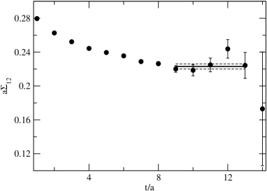
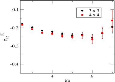
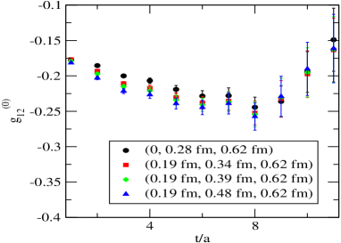
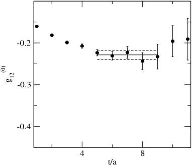
In order to reduce the statistical uncertainty in ratio (6), we have taken the asymptotic value of the energy splittings $\Sigma^{mn}_{\infty}=E_{n}-E_{m}$. We have shown in Figure 2 an example plateau for $\Sigma^{12}_{\infty}$. In addition we have set $t_{s}$ to $2t$ in (5). We have solved both $3\times 3$ and $4\times 4$ GEVP systems and checked the stability of the results when the local operator is included, as shown in Figure 3. Hereafter we will present results for a $3\times 3$ matrix of correlators with values of $r_{i}\equiv\{0.19\,\mathrm{fm},\,0.39\,\mathrm{fm},0.62\,\mathrm{fm}\}$. To check the dependence on $t_{0}$, to which the contribution from higher excited states is sensitive, we have both fixed it at a small value (typically, $2a$) and let it vary as $t-a$.

Figure 3: Dependence of bare $g_{12}$ on the size of the GEVP (left) and on the radius of wave functions (right) for the CLS ensemble E5.

CLS label	$\beta$	$L^{3}\times T$	$\kappa$	a [fm]	$m_{\pi}$ [MeV]	# of cnfgs
A5	5.2	$32^{3}\times 64$	0.13594	0.075	330	500
E5	5.3	$32^{3}\times 64$	0.13625	0.065	435	500
F6		$48^{3}\times 96$	0.13635		310	600
N6	5.5	$48^{3}\times 96$	0.13667	0.048	340	400

Table 2: Parameters of the simulations.

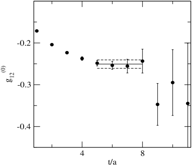
Though the uncertainty is a bit larger, we have confirmed the finding by BulavaYZ that using sGEVP (6) seems beneficial compared to the standard GEVP approach (5) to more strongly suppress contamination from higher excited states in the hadronic matrix element we measure. As illustrated in Figure 4, plateaux obtained from the GEVP and sGEVP are compatible: -0.25(1) for GEVP and -0.23(2) for sGEVP, with one additional point in the plateau of the sGEVP. Therefore, in the following we give results using the sGEVP only.

Figure 4: Plateaus of bare $g_{12}$ extracted by GEVP (left) and sGEVP (right) for the CLS ensemble E5.

After applying a non-perturbative procedure to renormalise the axial light-light current DellaMorteXB ; FritzschWQ , we are ready to extrapolate to the continuum limit. Inspired by Heavy Meson Chiral Perturbation Theory at leading order CasalbuoniPG ; BurdmanGH and due to the ${\cal O}(a)$ improvement of the three-point correlation functions (the improved part of the axial current, $ac_{A}\partial_{i}{\cal P}$, is absent at zero momentum), we apply two fit forms:

$$g_{12} = C_{0}+(a/a_{\beta=5.3})^{2}C_{1}+(m_{\pi}/m^{0}_{\pi})^{2}C_{2}\,,$$ (7)

$$g_{12} = C^{\prime}_{0}+(a/a_{\beta=5.3})^{2}C^{\prime}_{1}\,.$$ (8)

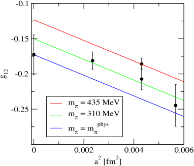
We show in Figure 5 the continuum extrapolation (7) of $g_{12}$. We observe quite large cut-off effects ($\sim 30\%$ at $\beta=5.3$), it is thus crucial to have several lattice spacings. We obtain finally, using (7) as the best estimate of the central value,

$$g_{12}=-0.17(3)(2)\,,$$ (9)

where the first error is statistical, and the second error corresponds to the chiral uncertainty that we evaluate from the discrepancy between (7) and (8).

Figure 5: Continuum and chiral extrapolation of $g_{12}$.

We collect in Table 3 the value of $g_{12}$ at each lattice point and at the physical point as well as the fit parameters for (7) and (8).

	$g_{12}$
A5	-0.245(29)
E5	-0.186(8)
F6	-0.207(15)
N6	-0.181(12)
physical point	-0.173(28)(18)

	fit (7)	fit (8)
$C_{0}$	-0.178(29)	-0.155(26)
$C_{1}$	-0.063(32)	-0.040(29)
$C_{2}$	0.0053(29)	-

Table 3: Value of $g_{12}$ at the lattice points and at the physical point (left) as well as the fit parameters of Eq. (7) and (8) (right).

	$a\Sigma_{12}$
A5	0.255(8)
E5	0.222(8)
F6	0.216(12)
N6	0.173(7)

Table 4: Mass splitting $\Sigma_{12}$ in lattice units. The error we quote is the discrepancy between plateaux that we extract for different time ranges {$[t_{\rm min},\,t_{\rm max}]$, $[t_{\rm min}\pm 0.2r_{0},\,t_{\rm max}\pm 0.2r_{0}]$}, where the Sommer scale $r_{0}$ SommerCE is about $0.5\,\mathrm{fm}$ FritzschWQ .

In simulations with light dynamical quarks, the onset of multi-hadron thresholds due to the emission of pions must be considered when examining excited $B$ meson properties. Such thresholds significantly complicate the extraction of hadron-to-hadron matrix elements from the two- and three-point correlation functions considered here. However with the $L<3\,\mathrm{fm}$ volumes in this work, the $P$-wave decay $B^{*^{\prime}}(\vec{0})\to B(\vec{p})\pi(-\vec{p})$ is kinematically forbidden. The $S$-wave decay $B^{*^{\prime}}\to B^{*}_{1}\pi$ is potentially more dangerous. Examining the mass splittings $\Sigma_{12}$ in Table 4, we notice that $630\,\mathrm{MeV}\lesssim\Sigma_{12}\lesssim 710\,\mathrm{MeV}$. If we assume that $400\,\mathrm{MeV}\lesssim m_{B^{*}_{1}}-m_{B}\lesssim 500\,\mathrm{MeV}$ in the pion mass range $[310\,\mathrm{MeV},\,440\,\mathrm{MeV}]$, (as has been found in a recent lattice study of the static light meson spectrum Michaelaa ), we conclude that our analysis is safe from these threshold effects. Moreover the bare couplings $g_{12}$ we obtain are similar to the quenched result of Ref. BulavaYZ .

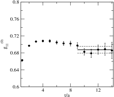
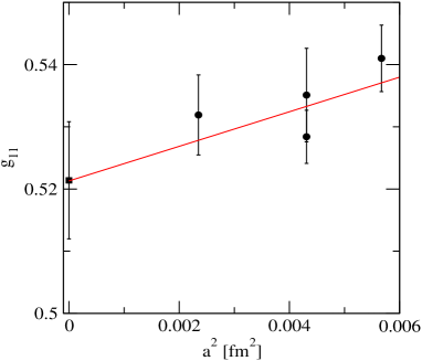
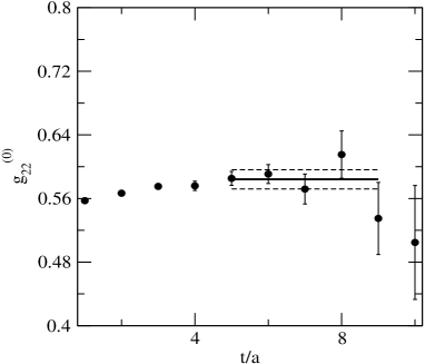
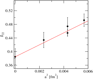
We show in Figure 6 a typical plateau of the bare coupling $g_{11}$ and the extrapolation to the continuum and chiral limit. That extrapolation is smooth, with a negligible dependence on $m_{\pi}$, and we obtain from the fit form (7) $g_{11}=0.52(2)$, in excellent agreement with a computation by the ALPHA Collaboration focused on that quantity BulavaEJ . We have added an error of 2% due to higher excited states which is estimated from plateaux at early times with a range ending at $\sim r_{0}$. Following the same strategy, we show in Figure 7 a typical plateau of the bare coupling $g_{22}$ and the extrapolation to the continuum and chiral limit, once again quite smooth, with an almost absent dependence on the sea quark mass. We obtain from the fit form (8) $g_{22}=0.38(4)$. Remarkably, the “diagonal” couplings $g_{11}$ and $g_{22}$ are significantly larger than the off-diagonal one $g_{12}$. This suggests that neglecting the contribution from $B^{\prime}$ mesons to the three-point light-cone sum rule used to obtain $g_{B^{*}B\pi}$ introduces uncontrolled systematics. Note that the decay constant $f_{B^{*^{\prime}}}$ itself is large compared to $f_{B}$ BurchQX ; BlossierMK . For completeness we have collected in Table 5 the value of $g_{11}$ and $g_{22}$ at each lattice point and at the physical point and the fit parameters of (7) and (8).

	$g_{11}$	$g_{22}$
A5	0.541(5)	0.492(19)
E5	0.535(8)	0.455(10)
F6	0.528(4)	0.474(26)
N6	0.532(6)	0.434(23)
physical point	0.516(12)(5)(10)	0.385(24)(28)

	$g_{11}$: fit (7)	$g_{11}$: fit (8)	$g_{22}$: fit (7)	$g_{22}$: fit (8)
$C_{0}$	0.515(13)	0.521(9)	0.416(27)	0.385(24)
$C_{1}$	0.012(9)	0.012(9)	0.074(25)	0.076(26)
$C_{2}$	0.0011(15)	-	-0.0033(33)	-

Table 5: Value of $g_{11}$ and $g_{22}$ at the lattice points and at the physical point (left) and fit parameters of eq. (7) and (8) (right). The third error on $g_{11}$ is an estimate of the effects of higher excited states.

Figure 6: Plateau of bare $g_{11}$ for the CLS ensemble E5 (left) and its extrapolation to the continuum and chiral limit (right).

IV Conclusion

We have performed a first estimate of the axial form factor $A_{1}(q^{2}_{\rm max})\equiv g_{12}$ parametrising at zero recoil the decay $B^{*^{\prime}}\to B$ in the static limit of HQET from ${\rm N_{f}=2}$ lattice simulations. Assuming the positivity of decay constants $f_{B}$ and $f_{B^{*^{\prime}}}$, we have obtained a negative value for this form factor. It is almost three times smaller than the $g_{11}$ coupling: $g_{12}=-0.17(4)$ while $g_{11}=0.52(2)$. Moreover we find $g_{22}=0.38(4)$, which is not strongly suppressed with respect to $g_{11}$. Our work is a first hint of confirmation of the statement made in Ref. BecirevicVP to explain the small value of $g_{D^{*}D\pi}$ computed analytically when compared to experiment. This computation using light-cone Borel sum rules may have been too naive. Following Ref. BecirevicYA , a next step in our general study of excited static-light meson states would be the measurement of $A_{1}(0)$ by computing the distribution in $r$ of the axial density $f_{A}(r)\equiv\langle B^{*^{\prime}}|\bar{\psi}_{l}\gamma^{i}\gamma^{5}\psi_{l}(r)|B\rangle$ and $A_{1}(0)=4\pi\,\int_{0}^{\infty}r^{2}f_{A}(r)e^{i\vec{q}\cdot\vec{r}}\,dr$.

Figure 7: Plateau of bare $g_{22}$ for the CLS ensemble E5 (left) and its extrapolation to the continuum and chiral limit (right).

Appendix

In this section we discuss the time dependence of $R^{\rm sGEVP}_{mn}$ (6). To simplify notation, we have fixed $a$ to 1. We have followed the strategy of Ref. BlossierKD to treat in perturbation theory the full GEVP, with an exact computation of the $N$ lowest states:

$$C^{(2)}_{ij}(t)=\langle\mathcal{O}_{i}(t)\mathcal{O}_{j}(0)\rangle=C_{ij}^{(2,0)}(t)+\epsilon C_{ij}^{(2,1)}(t)=\sum_{n=1}^{N}e^{-E_{n}t}\psi_{ni}\psi_{nj}+\sum_{n=N+1}^{\infty}e^{-E_{n}t}\psi_{ni}\psi_{nj}\,,$$

$$C^{(2)}(t)v_{n}(t,t_{0})=\lambda_{n}(t,t_{0})C^{(2)}(t_{0})v_{n}(t,t_{0})\,,$$

$$v_{n}(t,t_{0})=v_{n}^{(0)}(t,t_{0})+\epsilon v_{n}^{(1)}(t,t_{0})\,,$$

$$\lambda_{n}(t,t_{0})=\lambda_{n}^{(0)}(t,t_{0})+\epsilon\lambda_{n}^{(1)}(t,t_{0})\,.$$

Vectors are normalised such that

$$\langle v_{m}^{(0)},C^{(2,0)}(t_{0})v_{n}^{(0)}\rangle=\rho_{n}\delta_{nm}\,,$$

$$\langle v_{n}^{(1)},C^{(2,0)}(t_{0})v_{n}^{(0)}\rangle=0\,.$$

where $\rho_{n}=e^{-E_{n}t_{0}}$. Introducing the dual vectors $u_{n}$ defined by $\sum_{n=1}^{N}u_{ni}\psi_{mi}=\delta_{mn}$ $\forall n\leq N$, we note that

$$C^{(2,0)}(t)u_{n}=e^{-E_{n}t}\ \psi_{n},\quad v_{n}^{(0)}(t,t_{0})=u_{n},\quad\lambda_{n}^{(0)}(t,t_{0})=e^{-E_{n}(t-t_{0})}.$$

At first order in $\epsilon$, we have

$$\lambda_{n}^{(1)} =\rho_{n}^{-1}\left(v_{n}^{(0)},\Delta_{n}v_{n}^{(0)}\right)\,,$$

$$v_{n}^{(1)} =\sum_{m\neq n}v_{m}^{(0)}\rho_{m}^{-1}\frac{(v_{m}^{(0)},\Delta_{n}v_{n}^{(0)})}{\lambda_{n}^{(0)}-\lambda_{m}^{(0)}}=\sum_{n\neq m}\alpha_{nm}\ v_{m}^{(0)},$$

where $\Delta_{n}=C^{(2,1)}(t)-\lambda^{(0)}_{n}(t,t_{0})C^{(2,1)}(t_{0})$. With $c_{n,m,l}=\langle u_{n},\psi_{l}\rangle\langle u_{m},\psi_{l}\rangle$ we get:

$$\epsilon\frac{\lambda_{n}^{(1)}(t,t_{0})}{\lambda_{n}^{(0)}(t,t_{0})} =-\sum_{l>N}c_{n,n,l}e^{-(E_{l}-E_{n})t_{0}}\left[1-e^{-(E_{l}-E_{n})(t-t_{0})}\right]\,,$$

$$\epsilon\ \alpha_{nm}(t,t_{0}) =-\sum_{l>N}c_{n,m,l}\frac{1-e^{-(E_{l}-E_{n})(t-t_{0})}}{1-e^{-(E_{m}-E_{n})(t-t_{0})}}e^{-(E_{l}-E_{m})t_{0}}\,.$$

Finally the normalisation conditions read

$$\langle v_{n}(t,t_{0}),C(t_{0})v_{n}(t,t_{0})\rangle=\rho_{n}+\epsilon\langle v_{n}^{(0)},C^{(2,1)}(t_{0})v_{n}^{(0)}\rangle\,.$$

We are ready to develop (6) to first order in $\epsilon$:

$$\mathcal{M}_{mn}^{\mathrm{eff},s} = \partial_{t}\left\{\frac{\langle v_{m}(t,t_{0}),\left[K(t,t_{0})/\lambda_{n}(t,t_{0})-K(t_{0},t_{0})\right]v_{n}(t,t_{0})\rangle}{\left[\langle v_{m}(t,t_{0}),C^{(2)}(t_{0})v_{m}(t,t_{0})\rangle\langle v_{n}(t,t_{0}),C^{(2)}(t_{0})v_{n}(t,t_{0})\rangle\right]^{1/2}}e^{\frac{t_{0}}{2}\Sigma(t_{0},t_{0})}\right\}$$

$$= \mathcal{M}_{mn}^{\mathrm{eff},s,0}+\epsilon\mathcal{M}_{mn}^{\mathrm{eff},s,1},$$

$$\mathcal{M}_{mn}^{\mathrm{eff},s,0} =\partial_{t}\left\{\frac{\langle u_{m},\left[K(t,t_{0})/\lambda_{n}^{(0)}(t,t_{0})-K(t_{0},t_{0})\right]u_{n}\rangle}{\left[\langle u_{m},C^{(2)}(t_{0})u_{m}\rangle\langle u_{n},C^{(2)}(t_{0})u_{n}\rangle\right]^{1/2}}e^{\frac{t_{0}}{2}\Sigma(t_{0},t_{0})}\right\}.$$

With

$$\langle u_{m},K(t,t_{0})u_{n}\rangle=\sum_{t_{1}}e^{-\Sigma(t-t_{1})}\langle u_{m},C^{(3)}(t,t_{1})u_{n}\rangle=h_{mn}\ te^{-E_{n}t},\quad\langle u_{n},C^{(2)}(t_{0})u_{n}\rangle=\rho_{n}=e^{-E_{n}t_{0}}$$

we have at leading order

$$\mathcal{M}_{mn}^{\mathrm{eff},s,0}=h_{mn}.$$

The subleading order reads

$$\epsilon\mathcal{M}_{mn}^{\mathrm{eff},s,1}=\epsilon\partial_{t}\sum_{a=1}^{5}T_{a}.$$

$$T_{1}=-\frac{\lambda_{n}^{(1)}(t,t_{0})}{(\lambda_{n}^{(0)}(t,t_{0}))^{2}}\frac{\langle v_{m}^{(0)}(t,t_{0}),K(t,t_{0})v_{n}^{(0)}(t,t_{0})\rangle}{(\rho_{n}\rho_{m})^{1/2}}e^{\frac{t_{0}}{2}\Sigma(t_{0},t_{0})}=-\frac{\lambda_{n}^{(1)}(t,t_{0})}{\lambda_{n}^{(0)}(t,t_{0})}\langle v_{m}^{(0)}(t,t_{0}),K(t,t_{0})v_{n}^{(0)}(t,t_{0})\rangle e^{E_{n}t}\,.$$

The first subleading contribution is given by

$$T_{1}=-h_{mn}\ t\times\frac{\lambda_{n}^{(1)}(t,t_{0})}{\lambda_{n}^{(0)}(t,t_{0})}\sim c_{n,n,N+1}\ h_{mn}\times te^{-\Delta_{N+1,n}t_{0}}\left[1-e^{-\Delta_{N+1,n}(t-t_{0})}\right]\,.$$

Defining the discrete derivative $\partial_{t}A=A(t+1)-A(t)$, and taking at the end of the computation $t_{0}=t-1$, we get

$$\partial_{t}T_{1}\sim c_{n,n,N+1}\ h_{mn}\left(1-e^{-\Delta_{N+1,n}}\right)\times\left(t+1+e^{\Delta_{N+1,n}}\right)e^{-\Delta_{N+1,n}t}.$$

The second subleading contribution reads

$$T_{2}=\frac{\left(v_{m}^{(1)}(t,t_{0}),\left[K(t,t_{0})/\lambda_{n}^{(0)}(t,t_{0})-K(t_{0},t_{0})\right]v_{n}^{(0)}(t,t_{0})\right)}{(\rho_{n}\rho_{m})^{1/2}}e^{\frac{t_{0}}{2}\Sigma(t_{0},t_{0})}=\\ \sum_{p\neq m}\alpha_{mp}\ \langle v_{p}^{(0)}(t,t_{0}),\left[K(t,t_{0})e^{E_{n}t}-K(t_{0},t_{0})e^{E_{n}t_{0}}\right]v_{n}^{(0)}(t,t_{0})\rangle\,.$$

With some algebra, we deduce

$$\langle v_{p}^{(0)}(t,t_{0}),K(t,t_{0})v_{n}^{(0)}(t,t_{0})\rangle e^{E_{n}t} =\sum_{t_{1}}e^{-(t-t_{1})(E_{n}-E_{m})}\sum_{rs}\langle u_{p},\psi_{r}\rangle\langle\psi_{s},u_{n}\rangle h_{rs}e^{-E_{r}(t-t_{1})}e^{-E_{s}t_{1}}e^{E_{n}t}$$

$$=\sum_{t_{1}}e^{-(t-t_{1})(E_{n}-E_{m})}h_{pn}e^{-E_{p}(t-t_{1})}e^{-E_{n}t_{1}}e^{E_{n}t}$$

$$=\sum_{t_{1}}h_{pn}e^{-(E_{p}-E_{m})t_{1}},$$

and

$$\langle v_{p}^{(0)}(t,t_{0}),\left[K(t,t_{0})e^{E_{n}t}-K(t_{0},t_{0})e^{E_{n}t_{0}}\right]v_{n}^{(0)}(t,t_{0})\rangle =\sum_{t_{1}=t_{0}+1}^{t}h_{pn}e^{-(E_{p}-E_{m})t_{1}}.$$

Finally,

$$T_{2} =\sum_{p\neq m}\left[\alpha_{mp}(t,t_{0})\sum_{t_{1}=t_{0}+1}^{t}h_{pn}e^{-(E_{p}-E_{m})t_{1}}\right],$$

$$\partial_{t}T_{2}=\sum_{p\neq m}\left[\left(\alpha_{mp}(t+1,t_{0})-\alpha_{mp}(t,t_{0})\right)\sum_{t_{1}=t_{0}+1}^{t}h_{pn}e^{-(E_{p}-E_{m})t_{1}}+\alpha_{mp}(t+1,t_{0})\ h_{pn}e^{-(E_{p}-E_{m})(t+1)}\right]\,.$$

Setting $t_{0}=t-1$, the first term reads

$$\sum_{p\neq m}\left(\alpha_{mp}(t+1,t_{0})-\alpha_{mp}(t,t_{0})\right)\times e^{-(E_{p}-E_{m})t}\\ \sim-\sum_{p\neq m}\left[c_{m,p,N+1}e^{-(E_{N+1}-E_{p})(t-1)}\times\left(\frac{1-e^{-2(E_{N+1}-E_{m})}}{1-e^{-2(E_{p}-E_{m})}}-\frac{1-e^{-(E_{N+1}-E_{m})}}{1-e^{-(E_{p}-E_{m})}}\right)\right]\times h_{pn}e^{-(E_{p}-E_{m})t}\\ \sim-e^{-(E_{N+1}-E_{m})t}\sum_{p\neq m}\left[c_{m,p,N+1}h_{pn}e^{(E_{N+1}-E_{p})}\times\left(\frac{1-e^{-2(E_{N+1}-E_{m})}}{1-e^{-2(E_{p}-E_{m})}}-\frac{1-e^{-(E_{N+1}-E_{m})}}{1-e^{-(E_{p}-E_{m})}}\right)\right]\,,$$

and the second term reads

$$\sum_{p\neq m}\alpha_{mp}(t+1,t_{0})\ h_{pn}e^{-(E_{p}-E_{m})(t+1)}\\ \sim-\sum_{p\neq m}e^{-(E_{N+1}-E_{p})(t-1)}\frac{1-e^{-2(E_{N+1}-E_{m})}}{1-e^{-2(E_{p}-E_{m})}}c_{m,p,N+1}\ h_{pn}\times e^{-(E_{p}-E_{m})(t+1)}\\ \sim-e^{-(E_{N+1}-E_{m})t}\sum_{p\neq m}e^{(E_{N+1}+E_{m}-2E_{p})}\frac{1-e^{-2(E_{N+1}-E_{m})}}{1-e^{-2(E_{p}-E_{m})}}c_{m,p,N+1}\ h_{pn}.$$

We find

$$\partial_{t}T_{2}\sim\ e^{-(E_{N+1}-E_{m})t}\sum_{p\neq m}c_{m,p,N+1}h_{pn}\frac{1-e^{-(E_{N+1}-E_{m})}}{1-e^{-(E_{m}-E_{p})}}\,.$$

The third contribution

$$T_{3}=\frac{\left(v_{m}^{(0)}(t,t_{0}),\left[K(t,t_{0})/\lambda_{n}^{(0)}(t,t_{0})-K(t_{0},t_{0})\right]v_{n}^{(1)}(t,t_{0})\right)}{(\rho_{n}\rho_{m})^{1/2}}e^{\frac{t_{0}}{2}\Sigma(t_{0},t_{0})}$$

is obtained similarly to $\partial_{t}T_{2}$, permuting $m$ and $n$.
The fourth subleading contribution reads

$$T_{4} = \frac{1}{\lambda_{n}^{(0)}(t,t_{0})}\frac{\langle v_{m}^{(0)}(t,t_{0}),K^{(1)}(t,t_{0})v_{n}^{(0)}(t,t_{0})\rangle}{(\rho_{n}\rho_{m})^{1/2}}e^{\frac{t_{0}}{2}\Sigma(t_{0},t_{0})}=\langle v_{m}^{(0)}(t,t_{0}),K^{(1)}(t,t_{0})v_{n}^{(0)}(t,t_{0})\rangle e^{E_{n}t}\,.$$

With some algebra we deduce

$$\langle v_{m}^{(0)}(t,t_{0}),K^{(1)}(t,t_{0})v_{n}^{(0)}(t,t_{0})\rangle =\sum_{t_{1}}e^{-(E_{n}-E_{m})(t-t_{1})}\sum_{(r\,{\rm or}\,s)>N}\langle u_{m},\psi_{r}\rangle\langle\psi_{s},u_{n}\rangle h_{rs}e^{-E_{r}(t-t_{1})}e^{-E_{s}t_{1}}$$

$$\hskip 28.45274pt=\sum_{t_{1}}e^{-(E_{n}-E_{m})(t-t_{1})}\langle u_{m},\psi_{N+1}\rangle h_{N+1,n}e^{-E_{N+1}(t-t_{1})}e^{-E_{n}t_{1}}$$

$$\hskip 28.45274pt+\sum_{t_{1}}e^{-(E_{n}-E_{m})(t-t_{1})}\langle u_{n},\psi_{N+1}\rangle h_{N+1,m}e^{-E_{m}(t-t_{1})}e^{-E_{N+1}t_{1}}$$

$$\hskip 28.45274pt+\sum_{t_{1}}e^{-(E_{n}-E_{m})(t-t_{1})}\sum_{(r,s)>N}\langle u_{n},\psi_{r}\rangle\langle u_{m},\psi_{s}\rangle h_{r,s}e^{-E_{r}(t-t_{1})}e^{-E_{s}t_{1}}$$

$$\hskip 56.9055pt\sim\sum_{t_{1}}e^{-(E_{n}-E_{m})t_{1}}\langle u_{m},\psi_{N+1}\rangle h_{N+1,n}e^{-E_{N+1}t_{1}}e^{-E_{n}(t-t_{1})}$$

$$\hskip 56.9055pt+\sum_{t_{1}}e^{-E_{n}(t-t_{1})}\langle u_{n},\psi_{N+1}\rangle h_{N+1,m}e^{-E_{N+1}t_{1}}$$

$$\hskip 56.9055pt+\sum_{t_{1}}e^{-(E_{n}-E_{m})(t-t_{1})}\langle u_{n},\psi_{N+1}\rangle\langle u_{m},\psi_{N+1}\rangle h_{N+1,N+1}e^{-E_{N+1}t}$$

$$\hskip 85.35826pt\sim e^{-E_{n}t}\langle u_{m},\psi_{N+1}\rangle h_{N+1,n}\sum_{t_{1}}e^{-(E_{N+1}-E_{m})t_{1}}$$

$$\hskip 85.35826pt+e^{-E_{n}t}\langle u_{n},\psi_{N+1}\rangle h_{N+1,m}\sum_{t_{1}}e^{-(E_{N+1}-E_{n})t_{1}}$$

$$\hskip 85.35826pt+c_{n,m,N+1}\ h_{N+1,N+1}\ e^{-E_{N+1}t}\sum_{t_{1}}e^{-(E_{n}-E_{m})t_{1}}\,,$$

and we obtain

$$\partial_{t}T_{4}\sim +\langle u_{m},\psi_{N+1}\rangle h_{N+1,n}e^{-(E_{N+1}-E_{m})(t+1)}$$

$$+\langle u_{n},\psi_{N+1}\rangle h_{N+1,m}e^{-(E_{N+1}-E_{n})(t+1)}$$

$$-c_{n,m,N+1}h_{N+1,N+1}\frac{e^{-(E_{N+1}-E_{n})}-1}{e^{-(E_{n}-E_{m})}-1}e^{-(E_{N+1}-E_{n})t}$$

$$-c_{n,m,N+1}h_{N+1,N+1}\frac{e^{-(E_{N+1}-E_{m})}-1}{e^{-(E_{m}-E_{n})}-1}e^{-(E_{N+1}-E_{m})t}\,.$$

The last subleading contribution reads

$$T_{5} = -t\ h_{mn}\times\left(\frac{\langle v_{m}^{(0)},C^{(2,1)}(t_{0})v_{m}^{(0)}\rangle}{2\rho_{m}}+\frac{\langle v_{n}^{(0)},C^{(2,1)}(t_{0})v_{n}^{(0)}\rangle}{2\rho_{n}}\right)$$

$$\sim -t\ h_{mn}\times\left(\frac{1}{2}c_{m,m,N+1}e^{-(E_{N+1}-E_{m})t_{0}}+\frac{1}{2}c_{n,n,N+1}e^{-(E_{N+1}-E_{n})t_{0}}\right).$$

With $t_{0}=t-1$, we get

$$\partial_{t}T_{5}\sim-\frac{h_{mn}}{2}\times\left(c_{m,m,N+1}e^{-(E_{N+1}-E_{m})(t-1)}+c_{n,n,N+1}e^{-(E_{N+1}-E_{n})(t-1)}\right)$$

We see that for $n>m$ the dominating contribution $T_{1}$ to $\epsilon M^{{\rm eff},s,1}_{mn}$ is in $te^{-\Delta_{N+1,n}t}$ with subleading terms $T_{2}-T_{5}$ while for $n<m$ the leading contribution is in $e^{-(E_{N+1}-E_{m})t}$.

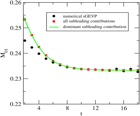
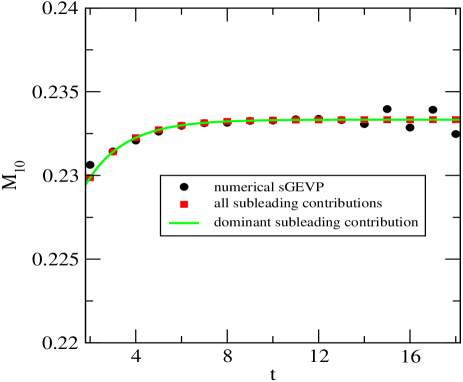
We have tested numerically our finding in the toy model of Ref. BulavaYZ , with $r_{0}E_{n}=n$, $r_{0}=0.3$, the $3\times 5$ matrix of couplings

$$\psi=\langle 0|\mathcal{O}_{i}|n\rangle=\begin{pmatrix}0.92&0.03&-0.10&-0.01&-0.02\\ 0.84&0.40&0.03&-0.06&0.00\\ 0.56&0.56&0.47&0.26&0.04\end{pmatrix},$$

and the hadronic matrix elements $M_{nn}=0.7\frac{6}{n+5}$, $M_{n,n+m}=\frac{M_{nn}}{3m}$. The comparison between the analytical formulae and the numerical solution is plotted in Figure 8. It is encouraging to obtain such good agreement after $t=8$.

Figure 8: Analytical formulae for $R^{\rm sGEVP}_{mn}$ compared to the numerical solution of our toy model.

References

• (1) P. Gambino, T. Mannel, and N. Uraltsev, JHEP 1210, 169 (2012), 1206.2296.
• (2) D. Becirevic et al., JHEP 0301, 009 (2003), hep-ph/0212177.
• (3) H. Ohki, H. Matsufuru, and T. Onogi, Phys.Rev. D77, 094509 (2008), 0802.1563.
• (4) D. Becirevic, B. Blossier, E. Chang, and B. Haas, Phys.Lett. B679, 231 (2009), 0905.3355.
• (5) ALPHA Collaboration, J. Bulava, M. Donnellan, and R. Sommer, PoS LATTICE2010, 303 (2010), 1011.4393.
• (6) W. Detmold, C. D. Lin, and S. Meinel, Phys.Rev. D85, 114508 (2012), 1203.3378.
• (7) D. Becirevic and F. Sanfilippo, Phys.Lett. B721, 94 (2013), 1210.5410.
• (8) ALPHA Collaboration, F. Bernardoni, J. Bulava, M. Donnellan, and R. Sommer, (In preparation).
• (9) R. Godang, (2013), 1301.0141.
• (10) A. Khodjamirian, R. Ruckl, S. Weinzierl, and O. I. Yakovlev, Phys.Lett. B457, 245 (1999), hep-ph/9903421.
• (11) J. Bulava, PoS LATTICE2011, 021 (2011), 1112.0212.
• (12) T. Burch et al., Phys.Rev. D74, 014504 (2006), hep-lat/0604019.
• (13) ALPHA Collaboration, B. Blossier et al., JHEP 1005, 074 (2010), 1004.2661.
• (14) D. Mohler and R. Woloshyn, Phys.Rev. D84, 054505 (2011), 1103.5506.
• (15) CSSM Lattice collaboration, M. S. Mahbub, W. Kamleh, D. B. Leinweber, P. J. Moran, and A. G. Williams, Phys.Lett. B707, 389 (2012), 1011.5724.
• (16) C. Michael, Nucl.Phys. B259, 58 (1985).
• (17) M. Luscher and U. Wolff, Nucl.Phys. B339, 222 (1990).
• (18) B. Blossier, M. Della Morte, G. von Hippel, T. Mendes, and R. Sommer, JHEP 0904, 094 (2009), 0902.1265.
• (19) J. Bulava, M. Donnellan, and R. Sommer, JHEP 1201, 140 (2012), 1108.3774.
• (20) A. Hasenfratz and F. Knechtli, Phys.Rev. D64, 034504 (2001), hep-lat/0103029.
• (21) M. Della Morte, A. Shindler, and R. Sommer, JHEP 0508, 051 (2005), hep-lat/0506008.
• (22) J. Foley et al., Comput.Phys.Commun. 172, 145 (2005), hep-lat/0505023.
• (23) S. Gusken et al., Phys.Lett. B227, 266 (1989).
• (24) APE Collaboration, M. Albanese et al., Phys.Lett. B192, 163 (1987).
• (25) M. Della Morte, R. Sommer, and S. Takeda, Phys.Lett. B672, 407 (2009), 0807.1120.
• (26) P. Fritzsch et al., Nucl.Phys. B865, 397 (2012), 1205.5380.
• (27) R. Casalbuoni et al., Phys.Rept. 281, 145 (1997), hep-ph/9605342.
• (28) G. Burdman and J. F. Donoghue, Phys.Lett. B280, 287 (1992).
• (29) R. Sommer, Nucl.Phys. B411, 839 (1994), hep-lat/9310022.
• (30) ETM Collaboration, C. Michael, A. Shindler, and M. Wagner, JHEP 1008, 009 (2010), 1004.4235.
• (31) T. Burch, C. Hagen, C. B. Lang, M. Limmer, and A. Schafer, Phys.Rev. D79, 014504 (2009), 0809.1103.
• (32) ALPHA Collaboration, B. Blossier et al., JHEP 1012, 039 (2010), 1006.5816.
• (33) D. Becirevic, E. Chang, and A. L. Yaouanc, Phys.Rev. D80, 034504 (2009), 0905.3352.