Temporal and spatial interference in molecular above-threshold ionization with elliptically polarized fields

Abstract

We investigate direct above-threshold ionization in diatomic molecules, with particular emphasis on how quantum interference is altered by a driving field of non-vanishing ellipticity. This interference may be either temporal, i.e., related to ionization events occurring at different times, or spatial, i.e., related to the electron emission at different centers in the molecule. Employing the strong-field approximation and saddle-point methods, we find that, in general, for non-vanishing ellipticity, there will be a blurring of the temporal and spatial interference patterns. The former blurring is caused by the electron velocity component perpendicular to the major polarization axis, while spatial interference is washed out as a consequence either of $s-p$ mixing, or of the temporal dependence of the ionization prefactor. Both types of interference are analyzed in detail in terms of electron trajectories, and specific conditions for which sharp fringes occur are provided.

I Introduction

Atoms and molecules interacting with a strong laser field may be ionized by absorbing more photons than necessary. This highly nonlinear phenomenon is called above-threshold ionization (ATI) and has attracted increasing attention since its 1979 discovery by Agostini and co-workers Agostini1979PRL . Recently, impressive progress has been achieved in the study of ATI. For example, great emphasis has been placed on employing ATI as a tool for the attosecond imaging of molecular orbitals Meckel2008Science ; Kang2010PRL . Imaging applications are based on the physical mechanism behind this phenomenon, in which the active electron (i) is released in the continuum, (ii) is accelerated by the field, and (iii) reaches the detector without returning or after rescattering with its parent molecule. The former and the latter scenario are known as direct ATI, and as rescattered or high-order ATI (HATI), respectively. Quantum mechanically, this electron may be released along several pathways, and the corresponding transition amplitudes will interfere.

Previous studies of ATI have shown that for the strong-field ionization of molecules, there are two kinds of quantum interference displayed in the ATI spectrum. In the first scenario, for a given energy, the electronic wave packet may reach the continuum at events occurring at different times in one cycle of laser field Becker2002AdvAtMolOptPhys . Hence, the transition amplitudes associated with ionization along different orbits in the time domain will interfere. This leads to a fringe structure in the ATI spectrum Milo2012PRA ; Bauer2005PRA , which is present regardless of whether the target is an atom or a molecule. For that reason, we will refer to this type of interference as “temporal interference”. Recently, ATI spectra with unusual two-photon separation in the direction perpendicular to the laser polarization Korneev2012PRL have been revealed due to the temporal interference.

In the second scenario, due to the multi-core structure of molecules, there may be electron emission from spatially separated centers, which results in a multi-slit like interference pattern in the ATI spectrum. In the context of linearly polarized fields and diatomic molecules, spatial-interference effects have been widely studied Fano1966PR ; Walter1999JPB ; Lei2002PRA ; selsto2005PRL ; Baltenkov2012JPB ; bohm2000PRL ; Busuladzic2008PRA ; Li2012PRA ; Carla2011PRA . Such studies range from simplified molecular models to exact three-dimensional time-dependent calculations. Employing the molecular strong-field approximation (SFA), a generalized spatial interference condition for diatomic molecules that accounts for the orbital geometry and $s-p$ mixing has been derived Busuladzic2008PRA ; Li2012PRA ; Carla2011PRA . For such fields, however, the dynamics are mainly confined along the field polarization axis.

Elliptically polarized laser fields exhibit a nonvanishing electric-field component perpendicular to the major polarization axis, which affects the motion of the electron in the laser field. Hence, they have been proposed as a resource for controlling strong-field phenomena by varying the ellipticity. For example, it is known that elliptical polarization has great significance as a tool to produce isolated attosecond pulses ottawa06 and to increase the contribution of long orbits in the HATI process Lai2013PRL . So far, the ellipticity dependence of ATI has been widely studied since the mid 1990s. Most studies, however, focus on the influence of the field ellipticity on the angular dependence of the ionization rate of ATI Eckle2008NatureP ; Busuladzic2009PRA ; Goreslavski2004PRL ; Staudte2009PRL , while the imprints left on the ATI spectrum by a nonvanishing driving-field ellipticity have received little attention.

In an early paper Paulus1998PRL , features related to the above-mentioned temporal interference have been identified experimentally for direct ATI. Therein, it was found that the photoelectron yield as a function of the driving-field ellipticity behaves in two very distinct ways for HATI and direct ATI energy ranges. While in the former case this yield decreases monotonically for larger driving field ellipticity, following the predictions of classical models, for direct ATI the electron ellipticity distributions display several “shoulder” structures. These structures have been related to the quantum temporal interference between the two sets of orbits that contribute to ATI in this energy region. However, how the ellipticity influences the two orbits still remains unexplored to a great extent.

In this work, we are interested in how the driving-field ellipticity influences the above-mentioned two kinds of interferences in the ATI spectra of diatomic molecules, exemplified by N₂ and Ar₂. Throughout, we focus on direct ATI, for which temporal interference effects are also prominent. Employing the molecular SFA and saddle-point methods, we find that, in general, the temporal interference in the ATI spectra will become blurred in the elliptically polarized field. For electron momenta along the major polarization axis, however, the temporal interference remains clear and the positions of the interference minima shift towards lower photoelectron energies with increasing ellipticity. These features are well explained in terms of the ellipticity dependence of the initial electron velocity along each orbit, and we show that the downshift of the interference minima is responsible for the “shoulder” structure observed in the ellipticity distributions of ATI electrons in Ref. Paulus1998PRL .

Furthermore, for the spatial interference, clear interference minima which do not depend on the ellipticity are found for N₂ if only $s$ or $p$ states are taken. However, if $s-p$ mixing is introduced, sharp fringes are only present for linear polarization if the molecule is aligned perpendicular to the field axis. For all other cases, these minima are blurred even for linear polarization. For Ar₂, the ATI spectra display several clear minima caused by the spatial interference. The reasons for the differences between N₂ and Ar₂ molecules are discussed in detail in terms of the shapes of their highest occupied molecular orbitals (HOMO). In this view, we propose a necessary condition to observe the spatial interference in the ATI spectrum in experiments.

This paper is organized as follows. In Sec. II, we provide a brief discussion of the model, including how to obtain the ATI amplitude and two-center interference conditions. Subsequently, we present the ATI spectra of the N₂ and Ar₂ molecules in the elliptically polarized laser field, and discuss how quantum interference is altered by the driving field of non-vanishing ellipticity. Finally, in Sec. IV our conclusions are given. Atomic units (a.u.) are used throughout unless otherwise indicated.

II Model

II.1 Transition Amplitude

Within the molecular SFA, the transition amplitude for direct ATI from the initial bound state $\left|\psi_{0}\right\rangle$ to a final Volkov state with drift momentum $\mathbf{p}$ is given by Carla2002PRA ; Becker2002AdvAtMolOptPhys ; KFR

$$M_{d}(\mathbf{p})=-i\int_{-\infty}^{\infty}dt\left\langle\mathbf{p}+\mathbf{A}(t)\right.|-\mathbf{r}\cdot\mathbf{E}(t)|\left.\psi_{0}\right\rangle\exp[iS_{d}(\mathbf{p},t)],$$ (1)

where

$$S_{d}(\mathbf{p},t)=-\frac{1}{2}\int_{t}^{\infty}[\mathbf{p}+\mathbf{A}(\tau)]^{2}d\tau+I_{p}t$$ (2)

is the semiclassical action. In Eqs. (1) and (2), $I_{p}$ gives the ionization potential, and $\mathbf{E}(t)$ and $\mathbf{A}(t)$ denote the laser electric field and the vector potential, respectively. For simplicity, we assume that all the molecular structure is contained in the ionization prefactor

$$d_{ion}=\left\langle\mathbf{p}+\mathbf{A}(t)\right.|-\mathbf{r}\cdot\mathbf{E}(t)|\left.\psi_{0}\right\rangle.$$ (3)

This is the most widespread assumption when performing the SFA modeling of strong-field phenomena in molecular systems (Carla2010PRA ; Milo2006PRA ; bohm2000PRL ; Madsen2004JPB ; Chu2005PRA ; see also the reviews Lein_Review ; Carla_Review ), and implies that the active electron leaves from the geometrical center of the molecule. In this work, we employ the single-active orbital approximation, i.e., we assume that the initial state $\left|\psi_{0}\right\rangle$ is the HOMO. This orbital is written as the linear combination of atomic orbitals (LCAO), and the core is assumed to be frozen. This latter approximation is reasonable for molecules with heavy nuclei Madsen2006 . Explicitly,

$$\psi_{0}(\mathbf{r})=\sum_{\alpha}c_{\alpha}\left[\psi_{\alpha}(\mathbf{r}+\frac{\mathbf{R}}{2})+(-1)^{l_{\alpha}-m_{\alpha}+\lambda_{\alpha}}\psi_{\alpha}(\mathbf{r}-\frac{\mathbf{R}}{2})\right],$$ (4)

where the wavefunctions $\psi_{\alpha}(\mathbf{r})$ give the atomic orbitals, $\mathbf{R}$ is the internuclear distance, $l_{\alpha}$ is the orbital quantum number, $m_{\alpha}$ is the magnetic quantum number and $\lambda_{\alpha}=m_{\alpha}$ for gerade (g) and $\lambda_{\alpha}=m+1$ for ungerade (u) orbital symmetry Wahl1964JCP .

II.2 Saddle-point equation and temporal interference

For sufficiently high intensity and low frequency of the laser field, the temporal integrations in the amplitude (1) can be mathematically evaluated by the saddle-point method with high accuracy Carla2002PRA ; Becker2002AdvAtMolOptPhys , i.e., we seek solutions such that the action (2) is stationary. For the specific case of an elliptically polarized field confined to the $xy$ plane, the saddle-point equation to be solved reads as

$$\frac{[p_{x}+A_{x}(t)]^{2}}{2}+\frac{[p_{y}+A_{y}(t)]^{2}}{2}+I_{p}=0,$$ (5)

where $p_{x}$ and $p_{y}$ denote the final momentum in the $\hat{\mathbf{x}}$ direction and in the $\hat{\mathbf{y}}$ direction, respectively. Physically, Eq. (5) ensures the conservation of energy at the ionization time $t$. In terms of the solutions $t_{s}$ of Eq. (5), the transition amplitude (1) can be written as

$$M_{d}(\mathbf{p})\propto\sum_{s}\mathcal{C}_{s}(t_{s})d_{ion}\exp[iS_{d}(\mathbf{p},t_{s})],$$ (6)

where the prefactors

$$\mathcal{C}_{s}(t_{s})=\sqrt{\frac{2\pi i}{\partial^{2}S_{d}(\mathbf{p},t_{s})/\partial t_{s}^{2}}}$$ (7)

are expected to vary much more slowly than the action at each saddle for the above-stated approximation to hold Bleistein . For each final momentum $\mathbf{p}$, there are two solutions of Eq. (5) within one period of the laser field, whose contributions will interfere. This interference is present regardless of whether the target has one or more centers, i.e., for atoms and molecules, and has been extensively studied in the literature for linearly polarized driving fields Korneev2012PRL ; Milo2012PRA ; Bauer2005PRA .

In this work, we employ the monochromatic elliptically polarized laser field

$$\mathbf{E}(t)=\frac{\omega A_{0}}{\sqrt{1+\xi^{2}}}(\hat{\mathbf{x}}\sin\omega t-\xi\hat{\mathbf{y}}\cos\omega t),$$ (8)

with vector potential

$$\mathbf{A}(t)=\frac{A_{0}}{\sqrt{1+\xi^{2}}}(\hat{\mathbf{x}}\cos\omega t+\xi\hat{\mathbf{y}}\sin\omega t),$$ (9)

where $\xi$ is the laser ellipticity. In this case, all cycles are equivalent and the amplitude $M_{d}(\mathbf{p})$ can be intuitively understood as the coherent superposition of the contributions of the two orbits, which may add constructively or destructively.  For vanishing electron momenta, these orbits will start at two consecutive maxima of the driving field $\mathbf{E}(t)$. These times will approach each other as the momentum increases. Throughout, we will refer to the orbits starting in the first and second half cycle of the field (8) as orbit 1 and orbit 2, respectively. For a discussion of these solutions for linearly polarized monochromatic fields see KopoldPhD ; SF2010 ; SFS2012 .

II.3 Spatial interference condition

Due to the two-center structure of the diatomic molecule, one may expect electron emission from spatially separated centers in the molecule. This results in minima and maxima in the ATI spectra, which, in the present model, are implicit in the ionization dipole matrix element $d_{ion}$. Using the length gauge with field-dressed molecular bound states DressedStates , the ionization prefactor (3) can be rewritten as

$$\begin{split}d_{ion}=-\sum_{\alpha}c_{\alpha}&[\exp(i\mathbf{p}\cdot\mathbf{R}/2)+(-1)^{l_{\alpha}-m_{\alpha}+\lambda_{\alpha}}\\ &\exp(-i\mathbf{p}\cdot\mathbf{R}/2)]\mathbf{E}(t)\cdot i\partial_{\tilde{\mathbf{p}}}\psi_{\alpha}(\tilde{\mathbf{p}})\end{split}$$ (10)

where $\psi_{\alpha}(\tilde{\mathbf{p}})$ is the Fourier transform of the atomic orbitals $\psi_{\alpha}(\mathbf{r})$ given by Eq. (4) with $\tilde{\mathbf{p}}=\mathbf{p}+\mathbf{A}(t)$. The two-center interference is related to the terms in the bracket in Eq. (10). This generalized interference condition accounts for $s-p$ mixing and the orbital geometry, and reduces to simpler interference conditions if only $s$ or $p$ states are present. For example, the terms in bracket reduce to $2\cos(\mathbf{p}\cdot\mathbf{R}/2)$ for $s$ states and gerade (g) symmetry. Thus, interference minima are present if

$$\mathbf{p}\cdot\mathbf{R}=(2k+1)\pi,$$ (11)

where $k$ denotes an integer number. Similarly, the interference minima are given by the condition

$$\mathbf{p}\cdot\mathbf{R}=2k\pi$$ (12)

for $p$ states and gerade symmetry. If, on the other hand, the HOMO has ungerade (u) symmetry, the above-stated scenario is reversed, i.e., the destructive interference condition for $p$ states is given by Eq. (11), while Eq. (12) holds for $s$ states.

In this paper, the molecular axis is kept in the plane $xy$ spanned by the driving-field ellipticity. The frame of reference ($\hat{\textbf{x}}^{\prime}$,$\hat{\textbf{y}}^{\prime}$,$\hat{\textbf{z}}^{\prime}$) of the molecule is rotated by an angle $\eta$ in this plane, defined with regard to the major polarization axis of the laser field. This means that $\hat{\textbf{x}}=\sin\eta\hat{\textbf{y}}^{\prime}+\cos\eta\hat{\textbf{x}}^{\prime}$, $\hat{\textbf{y}}=\cos\eta\hat{\textbf{y}}^{\prime}-\sin\eta\hat{\textbf{x}}^{\prime}$, and $\hat{\textbf{z}}=\hat{\textbf{z}}^{\prime}$.

The wave functions $\psi_{\alpha}(\mathbf{r})$ in Eq. (4) will be approximated by a Gaussian basis set

$$\psi_{\alpha}(\mathbf{r})=\sum_{v}b_{v}(x^{\prime})^{\beta_{x^{\prime}}}(y^{\prime})^{\beta_{y^{\prime}}}(z^{\prime})^{\beta_{z^{\prime}}}\exp(-\zeta_{v}r^{2}),$$ (13)

where the coefficients $c_{\alpha}$, $b_{v}$, $\beta_{x^{\prime},y^{\prime},z^{\prime}}$ and the exponents $\zeta_{v}$ are extracted from the quantum chemistry code GAMESS-UK GamessUK . Throughout, we employ a 6-31G basis so that only $s$ and $p$ states are considered. For a Gaussian basis set, the wave function $\psi_{\alpha}(\tilde{\mathbf{p}})$ in momentum space can be written as

$$\psi_{\alpha}(\tilde{\mathbf{p}})=\sum_{v}b_{v}\varphi_{v}(\tilde{\mathbf{p}}).$$ (14)

Usually, the explicit formula of $\varphi_{v}(\tilde{\mathbf{p}})$ is complicated. However, if only $s$ and $p$ states are used in the orbital construction, $\varphi_{v}(\tilde{\mathbf{p}})$ is simplified as

$$\varphi_{v}(\tilde{\mathbf{p}})=(-i\tilde{p}_{\chi})^{l_{\alpha}}\frac{\pi^{3/2}}{2^{l_{\alpha}}\zeta_{v}^{3/2+l_{\alpha}}}\exp[-\tilde{p}^{2}/(4\zeta_{v})],$$ (15)

where $l_{\alpha}=0,1$ and the subscript $\chi$ indicates the orientation of the $p$ states employed to construct the orbital. For instance, a $\sigma$ orbital would require $p$ states along the $\hat{\textbf{x}}^{\prime}$ axis, i.e., $\chi=x^{\prime}$, whereas a $\pi$ orbital would require $p$ states along the $\hat{\textbf{y}}^{\prime}$ or $\hat{\textbf{z}}^{\prime}$ axis, i.e., $\chi=y^{\prime}$ or $z^{\prime}$.

In this work, we will study the N₂ and Ar₂ molecules, both of which have $\sigma$ HOMOs. In combination with Eqs. (15) and (5), the prefactor in Eq. (10) can be specified as

$$\begin{split}d_{ion}&=i\cos(\frac{\mathbf{p}\cdot\textbf{R}}{2})\sum_{\alpha(s),v}c_{\alpha}b_{v}[\tilde{p}_{x}E_{x}(t)+\tilde{p}_{y}E_{y}(t)]\mathcal{D}_{s}+\\ &i\sin(\frac{\mathbf{p}\cdot\textbf{R}}{2})\sum_{\alpha(p),v}c_{\alpha}b_{v}\{[(\tilde{p}_{x}^{2}-2\zeta_{v})\cos\eta+\tilde{p}_{x}\tilde{p}_{y}\sin\eta]\times\\ &E_{x}(t)+[(\tilde{p}_{y}^{2}-2\zeta_{v})\sin\eta+\tilde{p}_{x}\tilde{p}_{y}\cos\eta]E_{y}(t)\}\mathcal{D}_{p}\end{split}$$ (16)

where $\mathcal{D}_{s}=e^{\frac{I_{p}}{2\zeta_{v}}}\pi^{3/2}/\zeta_{v}^{5/2}$ and $\mathcal{D}_{p}=e^{\frac{I_{p}}{2\zeta_{v}}}\pi^{3/2}/(2\zeta_{v}^{7/2}$). Note that, in Eq. (16), the momentum components relate to the electric field frame of reference.

III Results and discussion

In the results that follow, we will analyze how the above-mentioned temporal and spatial interference are influenced by a non-vanishing driving field ellipticity. This analysis will be performed in terms of electron orbits. For the temporal interference, we will focus on the N₂ molecule, which has been widely studied in the literature, both theoretically and experimentally. For all parameters employed in Sec. III.1, the structure caused by electron emission at separate centers gets washed out, so that temporal interference may be clearly assessed. In our studies of spatial interference effects (Sec. III.2), we consider the N₂ and Ar₂ molecules. Such molecules have very different HOMO geometries and equilibrium internuclear distances.

III.1 Temporal interference

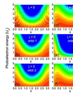
Figure 1: (Color online) ATI spectra of the N₂ molecule, coded in false colors in the ($E_{\mathbf{p}}$, $\theta$) plane and plotted in a logarithmic scale. In panels (a) and (d), both orbits 1 and 2 were included, for $\xi=0$ and $\xi=0.36$, respectively, while in panels (b), (c), (e) and (f) the contributions of individual orbits were taken. In panels (b) and (c), the field has been chosen to be linearly polarized ($\xi=0$), while in panels (e) and (f) the ellipticity is $\xi=0.36$. The major axis of the polarization ellipse is along the molecular axis, i.e., for alignment angle $\eta=0$. The laser intensity and wavelength are $I=2\times 10^{14}$ W/cm² and $\lambda=$800 nm, respectively.

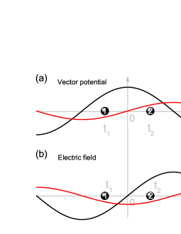
Figure 2: (Color online) Time evolution of the two components of the vector potential $\mathbf{A}(t)=\frac{A_{0}}{\sqrt{1+\xi^{2}}}(\hat{\mathbf{x}}\cos\omega t+\xi\hat{\mathbf{y}}\sin\omega t)$ and the electric field $\mathbf{E}(t)=\frac{\omega A_{0}}{\sqrt{1+\xi^{2}}}(\hat{\mathbf{x}}\sin\omega t-\xi\hat{\mathbf{y}}\cos\omega t)$, with $\xi=0.36$ [panels(a) and (b), respectively]. The two points $t_{1}$ and $t_{2}$ denote the times associated to the two ionization events $1$ and $2$ that occur within a field cycle, for an electron with the same final momentum $\mathbf{p}$. These events are indicated by the colored circles in the figure. For simplicity, we have defined the time related to a field crossing $E_{x}(t)=0$ for the electric-field component along the major polarization axis as $t=0$. This time also gives a maximum of the larger vector potential component $A_{x}(t)$. Note that $A_{x}(t_{1})=A_{x}(t_{2})$ as both events are equidistant in time from $t=0$.

Figure 1 shows the ATI spectra of the N₂ molecule, coded in false colors in the ($E_{\mathbf{p}}$, $\theta$) plane, where $\theta=\angle(\mathbf{R},\mathbf{p})$ denotes the angle between the internuclear distance and the drift momentum, and $E_{\mathbf{p}}=\mathbf{p}^{2}/2$ is the kinetic photoelectron energy upon reaching the detector, in units of the ponderomotive potential $U_{p}$. We assume that the major axis of the polarization ellipse is along the molecular axis, i.e., that the alignment angle $\eta=\angle(\mathbf{R},\mathbf{\hat{x}})$ is vanishing. For linear polarization [see Fig. 1(a)], many clear minima can be observed in the spectra. These minima are due to the destructive interference between orbit 1 and orbit 2. To illustrate this more clearly, we calculate the ATI transition probability density $|M_{d}(\mathbf{p})|^{2}$ employing only individual orbits, for the same parameters as in Fig. 1(a). These results are displayed in Figs. 1(b) and (c), and unambiguously show no minima.

With increasing ellipticity, the interference minima become blurred and, for most angles $\theta$, completely disappear as the ellipticity reaches $\xi=0.36$, as shown in Fig. 1(d). In fact, only the minima along and in the vicinity of the major polarization axis ($\theta=0$ and $\pi$) remain visible for this ellipticity. Sharp minima are only present exactly along the axis .

This behavior is due to the fact that, in general, a non-vanishing driving-field ellipticity affects the initial electron velocity along orbit 1 and orbit 2 unequally. The initial velocity of the electron at the ionization time $t$ is $\mathbf{p}+\mathbf{A}(t)$, and thus the velocity along the minor polarization axis is given by $v_{y}=p\sin\theta+A_{y}(t)$. In Fig. 2(a), we present the time evolution of the vector potential $\mathbf{A}(t)$ with ellipticity $\xi=0.36$. The two times $t_{1}$ and $t_{2}$ represent the ionization times related to orbit 1 and 2, respectively, and are equidistant from the electric field crossing $E_{x}(t)=0$ [see Fig. 2(b)]. The figure clearly shows that the directions of the vector potential $\mathbf{A}_{y}$ are opposite at the two ionization times. Thus if the electron leaves along orbit 1, the absolute value of its initial velocity $v_{y}$ should be larger than if it leaves along orbit 2. This holds except for linear polarization, i.e., if $A_{y}(t)\equiv 0$, or for electron momenta along the major polarization axis, i.e., for $\theta=0$ or $\pi$. The ionization rate at a specific ionization time $t$ is evaluated by $w(t,v_{0})=w_{0}(t)w_{1}(t,v_{0})$ Delone1991JOSA , where

$$w_{0}(t)=\frac{4(2I_{p})^{2}}{E(t)}\exp\left[-\frac{2}{3E(t)}(2I_{p})^{3/2}\right],$$ (17)

$$w_{1}(t,v_{0})=\frac{(2I_{p})^{2}}{E(t)\pi}\exp\left[-\frac{v_{0}^{2}}{E(t)}(2I_{p})^{1/2}\right],$$ (18)

and $v_{0}=\sqrt{v_{x}^{2}+v_{y}^{2}}$ is the initial velocity. Hence, the larger the initial velocity $v_{0}$ is, the lower the ionization rate at that ionization time will be. This implies that, for elliptical polarization, ionization along orbit 2 will become larger than ionization along orbit 1. Consequently, the destructive interference between two electron orbits will disappear in the ATI spectra. Here we assume that the transverse velocity of the electron is $p_{y}=p\sin\theta\leq 0$. If $p_{y}\geq 0$ the above-stated results are reversed.

This is in agreement with Figs. 1(e) and (f), in which we present the individual contributions to the ATI spectra from orbit 1 and orbit 2, respectively, for ellipticity $\xi=0.36$. In general, the probability density $|M_{d}(\mathbf{p})|^{2}$ associated with orbit 1 is much lower than that related to orbit 2. This is in stark contrast to what is observed for linear polarization, for which the two probability densities are identical [see Figs. 1(b) and (c)]. However, for drift momentum p along the major polarization axis ($\theta=0$ and $\pi$), the ATI probability densities are the same, because the two orbits exhibit the same initial perpendicular velocity $|v_{y}|=|A_{y}(t)|$. Therefore, the coherent superposition of the corresponding transition amplitudes will lead to clear interference minima in the ATI spectra, as observed in Fig. 1(d).

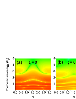
Figure 3: (Color online) ATI spectra of the N₂ molecule along the major polarization axis as a function of the alignment angle $\eta$, coded in false colors in the ($E_{\mathbf{p}}$, $\eta$) plane. Ellipticity $\xi=0$ for (a) and $\xi=0.36$ for (b). The parameters of the laser field are the same as in Fig. 1.

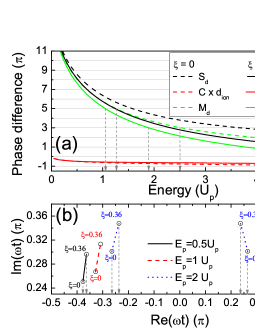
Figure 4: (Color online) (a) Phase difference between the contributions of the two orbits in Eq. (6) for parallel alignment $\eta=0$ and momentum along the major polarization axis ($\theta=0$) with $\xi=0$ (dashed lines) and $\xi=0.36$ (full lines): action (black), prefactor (red), and total transition amplitudes (green). The gray arrows indicate the values of the energy when the total phase difference is equal to $3\pi$ and $5\pi$ for $\xi=0$ and $\xi=0.36$. (b) Saddle points associated with the solutions of Eq. (5) for the two orbits as functions of the ellipticity from $\xi=0$ to $\xi=0.36$, for parallel alignment, momenta along the major polarization axis, and kinetic energies $E_{p}=0.5U_{p}$ (black full lines), $E_{p}=U_{p}$ (red dashed lines) and $E_{p}=2U_{p}$ (blue dotted lines). The gray arrows indicate the real values of the saddle points for $\xi=0$ and $\xi=0.36$.

Next we will further study the interference minima in the ATI spectra along the major polarization axis. In Fig. 3, we calculate the ATI spectra of the N₂ molecule with $\theta=0$ as a function of the alignment angle $\eta$. The most eye-catching features in the spectra are the clear minima due to the destructive interference between the two electron orbits. With increasing ellipticity, the ATI spectra seem to be squeezed and the positions of the minima are moving down to lower energies. For example, in Fig. 3(a) the position of one of the minima is about $2.5U_{p}$ for $\eta=0$ and $\xi=0$, but it becomes $1.9U_{p}$ in Fig. 3(b) for $\xi=0.36$. Furthermore, Fig. 3 shows that the downshift of the minima with the field ellipticity is much more dramatic for higher photoelectron energies than in the low-energy region.

In order to understand the behavior of the minima in Fig. 3, we calculate the phase difference between the two orbits in Eq. (6), which determines the positions of the interference minima in the ATI spectra. In Fig. 4(a), we exhibit the phase difference between the amplitudes $M^{(1)}_{d}(\mathbf{p})$ and $M^{(2)}_{d}(\mathbf{p})$, the actions $S_{d}(\mathbf{p},t_{1})$ and $S_{d}(\mathbf{p},t_{2})$, and the prefactors $\mathcal{C}_{1}(\mathbf{p},t_{1})d_{ion}^{(1)}$ and $\mathcal{C}_{2}(\mathbf{p},t_{2})d_{ion}^{(2)}$ associated with the two orbits for parallel alignment $\eta=0$, and field polarizations $\xi=0$ and $\xi=0.36$ (dashed and full lines, respectively). The figure shows that the phase difference between $S_{d}(\mathbf{p},t_{1})$ and $S_{d}(\mathbf{p},t_{2})$ (black lines) is smaller for $\xi=0.36$ than for $\xi=0$. This is caused by the real parts of two saddles $t_{1}$ and $t_{2}$ approaching each other for elliptical polarization , as illustrated in Fig. 4(b). Moreover, the approaching of the two saddles becomes more significant in the high-energy than in the low-energy region of the photoelectron spectra [see the gray arrows in Fig. 4(b)]. Therefore, the decrease of the phase difference associated with the action is much more dramatic for higher photoelectron energies than in the low-energy region. For the prefactor, the phase difference changes much less markedly with regard to the ellipticity, as shown in the red lines in Fig. 4(a). This is in agreement with the assumption of the steepest descent method that the prefactor varies more slowly with time than the action Bleistein . Thus, the change in the total phase difference [green lines in Fig. 4(a)] with the ellipticity is mainly determined by the action. When the difference in the total phase is equal to $(2k+1)\pi,k=0,1,2,...$, destructive interference between the two orbits will occur. In Fig. 4(a), the positions of the total phase difference with $k=1$ and $k=2$ are marked with arrows. The two positions are about $2.5U_{p}$ and $1.3U_{p}$ for linear polarization and move down to about $1.9U_{p}$ and $1.1U_{p}$, respectively, for elliptical polarization. Moreover, the downshift of the minima in the high-energy region is more significant than that in the low-energy region. These results are consistent with the behaviors of the interference minima observed in Fig. 3.

Furthermore, the behavior of the real parts of the saddle points in Fig. 4(b) can be explained in terms of the ellipticity dependence of the initial ionization velocity $v_{0}$. In the classical limit, the real parts $\mathrm{Re}(t_{1})$ and $\mathrm{Re}(t_{2})$ are associated with the classical ionization times $t_{1}$ and $t_{2}$ of an electron in the field (8), obtained if $I_{p}\rightarrow 0$. In a linearly polarized laser field, if an electron is released with drift momentum $\mathbf{p}$ along the major polarization axis, it will reach the continuum with the vanishing initial velocity $v_{0}=0$. In an elliptically polarized field, however, the electron should have a nonvanishing initial velocity in order to compensate the motion induced by the small component of the field. In the classical limit, the total initial velocity $\textbf{v}_{0}(t)$ of the electron is perpendicular to the laser electric field $\mathbf{E}(t)$ at the corresponding ionization time $t$ Goreslavski2004PRL ; Goreslavski1996ZETF , i.e., $\textbf{E}(t)\cdot\textbf{v}_{0}(t)=0$. The condition $\textbf{v}_{0}(t)\perp\mathbf{E}(t)$, $t=t_{1},t_{2}$ requires that $v_{x}(t_{1})>0$ and $v_{x}(t_{2})>0$ for the parameters employed in this paper. Since $v_{x}=p+A_{0}\cos\omega t_{1}/\sqrt{1+\xi^{2}}$ and $A_{x}(t)>0$ for both $t_{1}$ and $t_{2}$ [see Fig. 2(a)], an increase in the value of $v_{x}$ with the driving-field ellipticity requires that $t_{1}$ increases in order to approach the time for which $A_{x}(t)$ is maximal, i.e., $t=0$ [see Fig. 2]. Moreover, for the photoelectrons in the high energy region, the ionization time is closer to $t=0$ Becker2002AdvAtMolOptPhys . Hence, a larger initial velocity $v_{x}=-E_{y}/E_{x}v_{y}=\xi^{2}A_{0}\cos\omega t/\sqrt{1+\xi^{2}}$ will be required to satisfy the condition $\mathbf{v}_{0}\perp\mathbf{E}(t)$. This results in a larger increase of the ionization time. The same argument applies to orbit 2, with the difference that, because this orbit is located after the electric-field crossing [see Fig. 2(b)], $t_{2}$ should decrease. As a direct consequence, for increasing ellipticity the two ionization times should approach each other, and the approaching of the two times becomes more significant for higher photoelectron energies than in the low-energy region. These results are in good agreement with the two saddle-point solutions as functions of the driving-field ellipticity shown in Fig. 4(b) (or see Fig. 4 in Ref. Paulus1998PRL ).

It is worth mentioning that, because the interference minima in Fig. 3 move down to lower energy with increasing ellipticity, for fixed photoelectron energy there will be fluctuations in the ATI spectrum. This interesting phenomenon has been observed in experiments Paulus1998PRL and was called the “shoulder” structure in the ellipticity distribution of the ATI electrons. In our work, the underlying mechanism of the “shoulder” structure is explained in terms of the ellipticity dependence of the initial ionization velocity.

III.2 Two-center interference

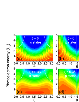
Figure 5: (Color online) ATI spectra of the N₂ molecule computed using only the s states [panels (a) and (c)] and the p states [panels(b) and (d)] from its HOMO, coded in false colors in the ($E_{\mathbf{p}}$, $\theta$) plane. The major axis of the polarization ellipse is along the molecular axis, $\eta=0$. Ellipticity $\xi=0$ for (a) and (c) and $\xi=0.36$ for (b) and (d). In all panels, the two-center interference minima are indicated by the white curves in the figure. The remaining field and molecular parameters are the same as in Fig. 1.

Finally, we will study the spatial interference due to electron emission at the two spatially separated centers in N₂ and Ar₂. The former molecule has a $3\sigma_{g}$ HOMO with a high degree of $s-p$ mixing. For the latter molecule, the HOMO is a $5\sigma_{u}$ orbital, in which the $p$ states dominate. Furthermore, Ar₂ exhibits a very large equilibrium internuclear distance ($R=7.2$ a.u.), so that, according to Eq. (10), several two center minima are expected to be present in the momentum range of interest.

In Fig. 5, we display the ATI spectra of N₂, if only the contributions from the $s$ or $p$ states to the HOMO are taken. These spectra are coded in false colors in the ($E_{\mathbf{p}}$, $\theta$) plane. The major axis of the polarization ellipse is chosen to be parallel to the molecular axis, i.e., at the alignment angle $\eta=0$. Fig. 5(a) shows that for the $s$-state contributions and linear polarization, apart from the minima caused by the temporal interference, there are other two minima, whose positions satisfy the two-center interference condition, Eq. (11), shown by the white lines in the figure. With increasing ellipticity [see Fig. 5(c)], the minima from the temporal interference are blurred as discussed in the previous section, but the minima from the two-center interference are still very clear. That is because the two-center interference condition, Eq. (11), is given for field-dressed initial bound states DressedStates . In this case, it is independent on the ellipticity. Similarly, for the $p$-state contributions, the two-center interference minima appear in the middle of the each panel in Figs. 5(b) and (d), because the corresponding electron momentum is perpendicular to the molecular axis, i.e., $\mathbf{p}\cdot\mathbf{R}=0$. Hence, the interference condition, Eq. (12), always holds.

However, when we consider the full $3\sigma_{g}$ HOMO of the N₂ molecule and include $s-p$ mixing, the minima from the two-center interference can not be observed in the ATI spectra. This holds for linearly and elliptically polarized fields, as shown in Figs. 1(a) and (d), and even if only the contributions of individual orbits are taken, as illustrated in Figs. 1(c), (b), (e), and (f). There are two main reasons for it. First, if $s-p$ mixing is included, the interference condition also depends on the sum of $\partial_{\tilde{\mathbf{p}}}\psi_{\alpha}(\tilde{\mathbf{p}})$ in Eq. (10), where $\tilde{\mathbf{p}}=\mathbf{p}+\mathbf{A}(t)$. This influence is expected to be considerable for $\mathrm{N}_{2}$, as its $3\sigma_{g}$ HOMO has a high degree of $s-p$ mixing. Second, the ionization time $t$ has a positive imaginary part, which can be related to the width of the barrier through which the electron must initially tunnel Becker2002AdvAtMolOptPhys . Thus, the sum in Eq. (10) is usually not purely real or imaginary, and therefore, the absolute value of Eq. (10) will never completely vanish, i.e., no clear minima will be observed in the ATI spectra.

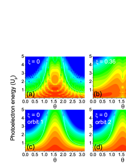
Figure 6: (Color online) (a) and (b) Logarithm of ATI spectra of the N₂ molecule, coded in false colors in the ($E_{\mathbf{p}}$, $\theta$) plane. The major axis of the polarization ellipse is perpendicular to the molecular axis, $\eta=\pi/2$. Ellipticity $\xi=0$ for (a) and $\xi=0.36$ for (b). (c) and (d) ATI spectra obtained by employing only individual orbits in the ($E_{\mathbf{p}}$, $\theta$) for $\xi=0$. The white curves indicate the minima caused by the two-center interference.

Nevertheless, there is a specific case in which clear spatial interference fringes are present in the full ATI spectra of N₂, if $s-p$ mixing is included. Fig. 6(a) shows the spectra for linear polarization with the alignment angle $\eta=\pi/2$. Apart from the minima from the temporal interference, there are two other minima. In order to show them more clearly, we calculate the ATI transition probability density $|M_{d}(\mathbf{p})|^{2}$ by employing only individual orbits to remove the pattern associated with the temporal interference. Figs. 6(c) and (d) display the ATI spectra without the temporal interference, where the clear minima from the spatial interference are observed. The reason for the appearance of the spatial interference in this specific case is that for the perpendicular alignment $\eta=\pi/2$ and for linear polarization, the ionization prefactor in Eq. (16) can be simplified as

$$\begin{split}d_{ion}=&i\cos(\frac{\mathbf{p}\cdot\textbf{R}}{2})\sum_{\alpha(s),v}c_{\alpha}b_{v}\tilde{p}_{x}E_{x}(t)\mathcal{D}_{s}+\\ &i\sin(\frac{\mathbf{p}\cdot\textbf{R}}{2})\sum_{\alpha(p),v}c_{\alpha}b_{v}\tilde{p}_{x}\tilde{p}_{y}E_{x}(t)\mathcal{D}_{p},\end{split}$$ (19)

where the momentum $\tilde{p}_{y}=p_{y}$ in the $\hat{\textbf{y}}$ direction is real. Thus, $i\tilde{p}_{x}E_{x}(t)$ can be factorized in both the first and the second terms in Eq. (19), and the remaining terms are time-independent and purely real. Using Eq. (19), we obtain the minima from the destructive spatial interference in the ATI spectra, shown by the white curves in Figs. 6(a), (c), and (d), which agree well with what is observed in the spectra. On the other hand, for elliptical polarization, the imaginary parts in the two terms in Eq. (16) are different. Hence, they cannot be factorized and the absolute value of Eq. (10) will never vanish. This is also the case if the field is linearly polarized, but $\eta\neq\pi/2$, as seen from Eq. (19). Fig. 6(b) shows that as the ellipticity increases to $\xi=0.36$, the minima from both the spatial and temporal interference in the spectra fade.

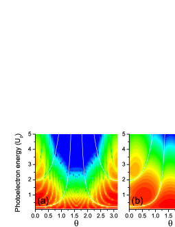
Figure 7: (Color online) ATI spectra of the Ar₂ molecule, with internuclear distance $R=7.2$ a.u., coded in false colors in the ($E_{\mathbf{p}}$, $\theta$) plane. The major axis of the polarization ellipse is along the molecular axis, $\eta=0$. The results in panels (a) and (b) have been computed for ellipticity $\xi=0$ and $\xi=0.36$, respectively. The minima caused by the two-center interference are indicated by white curves. The remaining field parameters are the same as in Fig. 1.

In contrast, the ATI spectra of the Ar₂ molecule present clear minima from the two-center interference, as seen in Fig. 7(a). In addition, Fig. 7(b) shows that, with increasing ellipticity, most minima from the temporal interference are blurred. However, the spatial minima remain unaltered. The critical reason for the difference between Ar₂ and N₂ molecules is that, in the $5\sigma_{u}$ HOMO of Ar₂, the contributions of the $p$ states dominate and the contributions of the $s$ states are practically vanishing for the internuclear separation in this work. Hence, the corresponding two-center interference condition is given by Eq. (11), which holds for pure $p$ states and ungerade symmetry. This condition, shown by the white lines in Fig. 7, is independent of the driving field and is consistent with the interference minima in the simulation. Furthermore, since Ar₂ has a very large equilibrium internuclear distance, $R=7.2$ a.u., several two-center minima are observed in the momentum range of interest according to Eq. (11).

IV Conclusions

In summary, we theoretically study temporal and spatial interference in the direct ATI spectra of aligned diatomic molecules in an elliptically polarized laser field. Temporal interference relates to ionization events occurring at different times within a field cycle, and spatial interference is associated with electron ionization at spatially separated centers in the molecule. Throughout, we have employed the molecular SFA, saddle-point methods and field-dressed bound states. We have also assumed that only the HOMO is active.

With increasing ellipticity, there will be a blurring of the temporal-interference patterns, except when the photoelectron momenta p are parallel to the major polarization axis. This blurring is caused by the fact that a nonvanishing driving field ellipticity affects the electron velocities unequally for the two ionization events occurring within each field cycle. For linear polarization, these events are equally probable. In order, however, to compensate the motion induced by the small component of the elliptically polarized field, it is necessary that, for one of the orbits, the electron be released in the continuum with a larger velocity. This will lead to a suppression of the corresponding ionization probability, and hence to a disappearance of the temporal interference patterns. Nevertheless, if the electron is released along the major polarization axis, the absolute value of the initial velocity will be the same for the two ionization events. Hence, the temporal-interference minima in the ATI spectrum will remain clear. For these specific parameters, we have analyzed in detail how a non-vanishing ellipticity shifts these minima towards lower energies, and have traced them to a decrease in the phase difference between the transition amplitudes related to both orbits. These results are in agreement with the studies performed in Paulus1998PRL .

Our results also show that, in general, the spatial, two center interference is much more robust with regard to the electric field parameters than the temporal interference, as long as the HOMO does not exhibit a high degree of $s-p$ mixing. As a consequence of $s-p$ mixing, however, or of the temporal dependence of the ionization prefactor Eq. (10), the interference patterns become blurred, even for linear polarization. Only for the very specific case of linear polarization and a molecule aligned perpendicular to the field direction will sharp fringes be observed. This is exemplified by computations in N₂. On the other hand, if either $s$ or $p$ states are dominant in the HOMO, the patterns will be very clear over a large parameter range and practically independent of the driving-field ellipticity. This is shown for the ATI spectra of Ar₂, which display clear spatial-interference patterns due to fact that the $p$-state contributions are dominant. Several minima exist due to the large equilibrium internuclear distance.

Therefore, one can trace all the interference patterns observed, or the absence thereof, to the dynamics of the electronic wave packet and the velocity with which it is released in the continuum. These patterns can be controlled by an appropriate choice of the the field and molecular parameters. Concrete examples provided in this work include the laser-field polarization, the molecular targets, the angle between the electron momentum and the major polarization axis, and the molecular orientation with regard to the field. This control is related to the energy position and to the sharpness of the patterns. We also identify a parameter region, for which clear interference fringes can be easily observed. We expect this information to be useful for future experiments.

V Acknowledgement

We are thankful to B. B. Augstein for his help with GAMESS-UK. This work has been funded by the UK EPSRC (grant EP/J019240/1), NNSF of China (grant No. 11204356), and the CAS overseas study and training program.

References

- (1) P. Agostini, F. Fabre, G. Mainfray, G. Petite, and N. K. Rahman, Phys. Rev. Lett. 42, 1127 (1979).
- (2) M. Meckel et al., Science 320, 1478 (2008).
- (3) H. Kang et al., Phys. Rev. Lett. 104, 203001 (2010).
- (4) W. Becker, F. Grasbon, R. Kopold, D. B. Milošević, G. G. Paulus, and H. Walther, Adv. At. Mol. Opt. Phys. 48, 35 (2002).
- (5) M. Busuladžić and D. B. Milošević, Phys. Rev. A 82, 015401 (2010).
- (6) D. Bauer, D. B. Milošević, and W. Becker, Phys. Rev. A 72, 023415 (2005).
- (7) Ph. A. Korneev et al., Phys. Rev. Lett. 108, 223601 (2012).
- (8) H. D. Cohen and U. Fano, Phys. Rev. 150, 30 (1966).
- (9) M. Walter and J. Briggs, J. Phys. B 32, 2487 (1999).
- (10) M. Lein, J. P. Marangos, and P. L. Knight, Phys. Rev. A 66, 051404(R) (2002).
- (11) S. Selstø, M. Førre, J. P. Hansen, and L. B. Madsen, Phys. Rev. Lett. 95, 093002 (2005).
- (12) A. S. Baltenkov, U. Becker, S. T. Manson, and A. Z. Msezane, J. Phys. B 45, 035202 (2012).
- (13) J. Muth-Böhm, A. Becker, and F. H. M. Faisal, Phys. Rev. Lett. 85, 2280 (2000).
- (14) M. Busuladžić. A. Gazibegović-Busuladžić, D. B. Milošević, and W. Becker, Phys. Rev. A 78, 033412 (2008).
- (15) T. Shaaran, B. B. Augstein, and C. Figueira de Morisson Faria, Phys. Rev. A 84, 013429 (2011).
- (16) W. Li and J. Liu, Phys. Rev. A 86, 033414 (2012).
- (17) N. Dudovich, J. Levesque, O. Smirnova, D. Zeidler, D. Comtois, M. Yu. Ivanov, D. M. Villeneuve, and P. B. Corkum, Phys. Rev. Lett. 97, 253903 (2006).
- (18) X. Y. Lai et al., Phys. Rev. Lett. 110, 043002 (2013).
- (19) P. Eckle et al., Nature Phys. 4, 565 (2008).
- (20) S. P. Goreslavski, G. G. Paulus, S. V. Popruzhenko, and N. I. Shvetsov-Shilovski, Phys. Rev. Lett. 93, 233002 (2004).
- (21) A. Staudte et al., Phys. Rev. Lett. 102, 033004 (2009).
- (22) M. Busuladžić. A. Gazibegović-Busuladžić, and D. B. Milošević, Phys. Rev. A 80, 013420 (2009).
- (23) G. G. Paulus, F. Zacher, H. Walther, A. Lohr, W. Becker and M. Kleber, Phys. Rev. Lett. 80, 484 (1998).
- (24) C. Figueira de Morisson Faria, H. Schomerus, and W. Becker, Phys. Rev. A 66, 043413 (2002).
- (25) L. V. Keldysh, Zh.Eksp. Teor. Fiz. 47, 1945 (1964) [Sov. Phys. JETP 20, 1307 (1965)]; F. H. M. Faisal, J. Phys. B 6, L89 (1973); H. R. Reiss, Phys. Rev. A 22, 1786 (1980).
- (26) C. Figueira de Morisson Faria and B. B. Augstein, Phys. Rev. A 81, 043409 (2010).
- (27) D. B. Milošević, Phys. Rev. A 74, 063404 (2006).
- (28) T. K. Kjeldsen and L. B. Madsen, J. Phys. B 37, 2033 (2004).
- (29) V. I. Usachenko and Shih-I. Chu, Phys. Rev. A 71, 063410 (2005).
- (30) M. Lein, J. Phys. B 40, R135 (2007).
- (31) B. B. Augstein and C. Figueira de Morisson Faria, Modern Phys. Lett. B 26, 1130002 (2011).
- (32) C. B. Madsen and L. B. Madsen, Phys. Rev. A 74, 023403 (2006)
- (33) A. C. Wahl, J. Chem. Phys. 41, 2600 (1964).
- (34) GAMESS-UK is a package of ab initio programs. See http://www.cfs.dl.ac.uk/gamess-uk/index.shtml, M. F. Guest, I. J. Bush, H. J. J. van Dam, P. Sherwood, J. M. H. Thomas, J. H. van Lenthe, R. W. A. Havenith, J. Kendrick, Mol. Phys. 103, 719 (2005).
- (35) N. Bleistein and R. A Handelsman, “Asymptotic Expansions of Integrals” (Dover, New York, 1975)
- (36) R. Kopold, PhD thesis, Technical University Munich, Chapt. 5 (2001).
- (37) T. Shaaran and C. Figueira de Morisson Faria, J. Mod. Opt. 57, 984 (2010); T. Shaaran, M. T. Nygren, and C. Figueira de Morisson Faria, Phys. Rev. A 81, 063413 (2010).
- (38) T. Shaaran, C. Figueira de Morisson Faria, and H. Schomerus, Phys. Rev. A 85, 023423 (2012).
- (39) D. B. Milošević, Phys. Rev. A 74, 063404 (2006); W. Becker, J. Chen, S. G. Chen, and D. B. Milošević, Phys. Rev. A 76, 033403 (2007).
- (40) N. B. Delone and V. P. Krainov, J. Opt. Soc. Am. B 8, 1207 (1991).
- (41) S. P. Goreslavski and S. V. Popruzhenko, Zh. Eksp. Teor, Fiz. 110, 1200 (1996) [Sov. Phys. JETP 83, 661 (1996)].