Testing OPE for ghosts, gluons and $\alpha_{s}$

Abstract:

We present here our results on extracting Wilson coefficients from different quantities such as ghost and gluon propagators which are calculated by means of Lattice QCD. The results confirm the validity of our method for the calculation of the strong coupling constant as well as allow to estimate the range of momenta where OPE is applicable.

1 Introduction

It can be argued that the strong coupling constant $\alpha_{s}$, or, equivalently, the QCD scale $\Lambda_{QCD}$ are the fundamental quantities which require a high level of precision as they enter in most calculations, both perturbative and non-perturbative. They can be extracted both from experiment or numerically, with the help of Lattice QCD. The latter is a complicated procedure and it is imperative to understand the underlying mechanics to estimate correctly the systematic errors. For the review of such calculations see, for instance, [1, 2, 3, 4, 5, 6, 7]. We presented our most recent results in [8] and here we will demonstrate that our approach and estimation of systematics is justified.

The work is based on ghost and gluon propagators, which we recently computed on the gauge configurations produced by the ETM Collaboration. These are the first to incorporate the effects of dynamical charm quarks. In other words, this is an ensemble of sample gauge fields including $N_{f}$=2+1+1, two light degenerate and two heavy, dynamical quark flavours (see [9, 10] for details of the simulations setup) with a twisted-mass fermion action [11, 12]. Combining the propagators in Taylor scheme we were able to extract the strong coupling constant, which agrees pretty well with the experimental results from $\tau$ decays [13] and ”world average” from PDG [14] at all scales from $\tau$ to $Z_{0}$. At the same time it became clear that invocation of nonperturbative OPE corrections is unequivocally needed to account properly for the lattice data of the coupling in Taylor scheme. Within the OPE procedure we expand matrix elements of any non-local operator in terms of local operators, organized by their momentum dimensions. Using the sum rules factorization [15, 16], these can be expressed as a coefficient to be computed in perturbation (Wilson coefficient) and the nonperturbative condensate of a local operator. For such procedure to be consistent it is required that (up to a proper renormalization constant for the local operator) the value of the condensate should be the same for any Green Function.

In refs. [17, 18] for $N_{f}$=2+1+1 and in refs. [7, 19] for $N_{f}$=0 and $N_{f}=$2 quark flavours respectively, we calculate the running coupling by equating numerical results and the OPE prediction. The OPE is clearly dominated by the landau gauge gluon condensate $A^{2}$ which has been elsewhere very much studied (e.g., see [20, 21, 22, 23, 24, 25, 26]). It can be noted that to calculate the coupling more reliably we combined the bare lattice propagators in such a manner that the cut-off dependence is minimal, which prevents the check for the universality of condensates, as gluon and ghost propagators are not to be independently analyzed. However our previous studies in quenched approximation suggested that such universality (even including the three-gluon vertex) is indeed compatible with the numerical data ($N_{f}$=0) [20, 27, 28, 6, 29, 7]. This has been also supported by the calculations with $N_{f}$=2 dynamical flavours [19, 30]. Now we will address this question in the $N_{f}=$2+1+1 case, to clarify the nature itself of the unavoidable nonperturbative corrections and the involved condensates.

2 Basics and Simulations

The Taylor coupling can be obtained directly from the gluon and ghost dressing functions it follows [7],

$$\alpha_{T}(p^{2})\ =\ \frac{g_{0}^{2}(a^{-1})}{4\pi}\ F^{2}(p^{2},a^{-1})\ G(p^{2},a^{-1})\ .$$ (1)

Substituting the dressing functions by their OPE expressions we are left with

$$\alpha_{T}(p^{2})\ =\ \alpha_{T}^{\rm pert}(p^{2})\left(1+9\ R\left(\alpha_{T}^{\rm pert}(p^{2}),\alpha_{T}^{\rm pert}(\mu^{2})\right)\left(\frac{\alpha(p^{2})}{\alpha(\mu^{2})}\right)^{\frac{27}{100}}\ \frac{g^{2}(\mu^{2})\langle A^{2}\rangle_{{\rm R},\mu^{2}}}{4\left(N^{2}_{c}-1\right)p^{2}}\ +\ \cdots\right)$$ (2)

where $R$ is known to four loops.

We refer to the upcoming paper [31] for the details of this calculation.

The ghost and gluon propagators are defined as follows:

$$\Delta^{ab}_{\mu\nu}(q) = \left\langle A_{\mu}^{a}(q)A_{\nu}^{b}(-q)\right\rangle=\delta^{ab}\left(\delta_{\mu\nu}-\frac{q_{\mu}q_{\nu}}{q^{2}}\right)\frac{G(q^{2})}{q^{2}}\;,$$

$$F^{ab}(q^{2}) = \frac{1}{V}\ \left\langle\sum_{x,y}\exp[iq\cdot(x-y)]\left(M^{-1}\right)^{ab}_{xy}\right\rangle=\delta^{ab}\frac{F(q^{2})}{q^{2}}\;;$$ (3)

where $A_{\mu}^{a}$ is the gauge field and $M^{ab}\equiv\partial_{\mu}D^{ab}_{\mu}$ is the Fadeev-Popov operator.The lattice setup is described in [18] and summarized in Tab. 1. The $O(4)$-breaking lattice artefacts have been cured by the so-called $H(4)$-extrapolation procedure [3, 32]. These estimates for bare gluon and ghost dressing functions appear plotted in Fig. 1.

$\beta$	$\kappa_{\rm crit}$	$a\mu_{l}$	$a\mu_{\sigma}$	$a\mu_{\delta}$	$(L/a)^{3}\times T/a$	confs.
1.90	0.1632700	0.0040	0.150	0.1900	$32^{3}\times 64$	50
1.95	0.1612400	0.0035	0.135	0.1700	$32^{3}\times 64$	50
2.10	0.1563570	0.0020	0.120	0.1385	$48^{3}\times 96$	100

Table 1: Lattice setup parameters for the ensembles we used in this paper: $\kappa_{\rm crit}$ is the critical value for the standard hopping parameter for the bare untwisted mass; $\mu_{l}$ stands for the twisted mass for the two degenerated light quarks, while $\mu_{\sigma}$ and $\mu_{\delta}$ define the heavy quarks twisted masses; the last column indicates the number of gauge field configurations exploited. This implies that the strange quark mass is roughly set to 95 MeV and the charm one to 1.51 GeV (in $\overline{\mbox{{\sc ms}}}$ at 2 GeV), while degenerate light quark masses range from 20 to 50 MeV (The lightest pseudoscalar masses approximately range from 270 to 510 MeV).

3 Testing the OPE

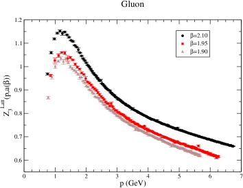
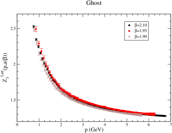
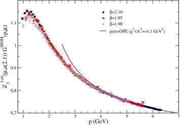
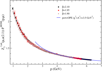
Figure 1: Bare gluon and ghost propagators as they result from lattice computations before (top) and after being cured of $O(4)$-invariant lattice artefacts and properly rescaled to appear superimposed (bottom). The blue solid line correspond to the best fit with the OPE formula.

The gluon and ghost propagator lattice data shown in the upper plots of Fig. 1 are still affected by $O(4)$-invariant lattice artefacts. As we did in ref. [17, 18, 30] for the Taylor coupling and the vector quark propagator, the gluon propagator renormalization constant $Z_{3}^{\rm Latt}$ in MOM scheme can be written as

$$Z_{3}^{\rm Latt}(p^{2},a^{-1})\ =\ G(p^{2},a^{-1})+c_{a2p2}\ a^{2}p^{2}\ ,$$ (4)

which corresponds to the lattice gluon dressing function. In r.h.s., the artefacts-free gluon dressing is noted as $G$. It can be shown that we can rewrite Eq. (4) as:

$$\frac{Z_{3}^{\rm Latt}(p^{2},a^{-1})}{G^{\rm NP}\left(\frac{p^{2}}{\mu^{2}},\alpha(\mu^{2})\right)}\ =\ z(\mu^{2},a^{-1})\ +\ c_{a2p2}\ \frac{a^{2}p^{2}}{G^{\rm NP}\left(\frac{p^{2}}{\mu^{2}},\alpha(\mu^{2})\right)}$$ (5)

with

$$G^{\rm NP}\left(\frac{p^{2}}{\mu^{2}},\alpha(\mu^{2})\right)\ =\ G_{0}^{\mbox{{\sc mom}}}\left(\frac{p^{2}}{\mu^{2}},\alpha(\mu^{2})\right)\left(1+C_{w}\left(\frac{p^{2}}{\mu^{2}},\alpha(\mu^{2})\right)\ \frac{\langle A^{2}\rangle_{{\rm R},\mu^{2}}}{4\left(N^{2}_{c}-1\right)p^{2}}\ +\ \cdots\ \right),$$ (6)

where Wilson coefficient $C_{w}\left(\frac{p^{2}}{\mu^{2}},\alpha(\mu^{2})\right)$, in the appropriate renormalization scheme, is known at the four-loop order with the help of the perturbative expansions for the gluon propagator MOM anomalous dimension and Taylor scheme beta function [33]. $G^{\rm NP}$ is expected to describe properly the nonperturbative running of the gluon dressing from lower bound of $p=4.5$ GeV, below which the lattice data deviate from the nonperturbative prediction only including the OPE leading power correction, to the upper bound of $a^{2}p^{2}\sim 3.5$, above where the impact of higher-order lattice artefacts cannot be neglected any longer. Now we can perform a linear fit and determine the overall factor, $z(\mu,a^{-1})$, for each data set and the coefficients $c_{\rm a2p2}$, which should be almost the same as they depend only logarithmically on the lattice spacing $a(\beta)$ by dimensional arguments (see tab. 2). This way we can remove the $O(4)$-invariant artefacts away from the lattice data for all available momenta in the aforementioned range, by applying Eq. (4), to be left with the continuum nonperturbative running for the gluon dressing; while the overall factors $z(\mu,a^{-1})$ can be used to rescale the data obtained at different $\beta$ such that they all will follow the same curve (see down plots of fig. 1).

As $G^{\rm NP}$ depends on $\Lambda_{\overline{\rm MS}}$ and the gluon condensate, $g^{2}\langle A^{2}\rangle$, their values have to be known prior to the removal of $O(4)$-invariant artefacts. In practice, we will take $\Lambda_{\overline{\rm MS}}$ to be known from $\tau$ decays ($\alpha_{\overline{\mbox{{\sc ms}}}}(m_{\tau}^{2})=0.334(14)$ [13], i.e. $\Lambda_{\overline{\rm MS}}=311$ MeV for $N_{f}=4$) and will search for a value of $g^{2}\langle A^{2}\rangle$ such that one gets the best matching of the rescaled gluon dressings from the three data sets. The details and the intermediate results of this procedure will be explained in [31]. Here we just present the results in Tab. 3.

	gluon	ghost
$g^{2}\langle A^{2}\rangle$ [GeV2]	4.7	3.2
$\beta$   $z(\mu^{2},a^{-1})$ $c_{a2p2}$	2.10 1.95 1.90 0.6495(5) 0.6068(26) 0.5971(30) -0.0097(2) -0.0071(8) -0.0080(8)	2.10 1.95 1.90 1.215(6) 1.229(20) 1.193(31) 0.0002(19) -0.0012(44) 0.0011(69)
$g^{2}\langle A^{2}\rangle$ [GeV2]	4.1	4.1
$z(\mu^{2},a^{-1})$   $c_{a2p2}$	0.6531(5) 0.6106(26) 0.6014(30) -0.0104(2) -0.0077(8) -0.0086(8)	1.206(6) 1.218(19) 1.182(30) 0.0022(19) 0.0004(44) 0.003(7)

Table 2: The overall factors, $z(\mu^{2},a^{-1})$, and the coefficients $c_{a2p2}$, for optimal values of $g^{2}\langle A^{2}\rangle$. As discussed there, $c_{a2p2}$ is thought not to depend very much on $\beta$ and so is fairly obtained from the results shown here. The renormalization point, $\mu$, for the overall factor is fixed at 10 GeV. Statistical errors have been computed by applying the Jackknife method.

	gluon	ghost	$\alpha_{T}$ [17]	$\alpha_{T}$ [18]
$g^{2}\langle A^{2}\rangle$ [GeV2]	4.7(1.6)	3.1(1.1)	4.5(4)	3.8(1.0)

Table 3: Results for $g^{2}\langle A^{2}\rangle$ independently obtained from gluon and ghost propagators in this paper and from the Taylor coupling analysis in refs. [17, 18].

Finally, one can impose the condensates to be the same for both gluon and ghost propagators, which leads to $g^{2}\langle A^{2}\rangle=4.1$ GeV², that appears to be again in a pretty good agreement with the previous results in refs. [17, 18]. In the following, we will use the artefacts-free gluon and ghost dressing functions, obtained with this last value for the gluon condensate, shown in Fig. 1.

Now we can directly test the validity of the OPE to describe consistently and accurately different Green functions by confronting the directly extracted numbers with theoretical predictions:

$$p^{2}\ \left[\frac{G(p^{2},a^{-1})}{z(\mu^{2},a^{-1})}-G^{\rm MOM}_{0}\left(\frac{p^{2}}{\mu^{2}},\alpha(\mu^{2})\right)\right]\ =\ G^{\rm MOM}_{0}\left(\frac{p^{2}}{\mu^{2}},\alpha(\mu^{2})\right)C_{w}\left(\frac{p^{2}}{\mu^{2}},\alpha(\mu^{2})\right)\frac{\langle A^{2}\rangle_{{\rm R},\mu^{2}}}{4\left(N^{2}_{c}-1\right)}\ ,$$ (7)

where the l.h.s. is computed after the removal of the artefacts.

On Eq. (7)’s r.h.s., the running with momenta can be easily expressed as a perturbative series in terms of the Taylor coupling, being proportional to the gluon condensate, $g^{2}\langle A^{2}\rangle$, which we already calculated. As one can see from the Fig. 2, the nonperturbative corrections are totally unavoidable for both the gluon (top) and ghost (bottom) cases. Also, the Wilson coefficient derived at the order ${\cal O}(\alpha^{4})$ in sec. 2 gives a high-quality fit of data (blue solid lines in both plots). Had we not included the Wilson coefficient running (i.e., dropped $C_{w}$ from Eq. (7)’s r.h.s.), or just included its leading logarithm approximation, a flatter slope would be obtained, not describing properly the data (blue dotted and green solid lines). A similar situation can be observed in the case of Taylor coupling itself, see Fig.3.

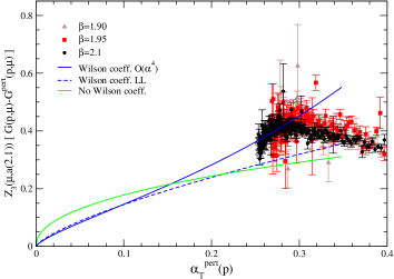
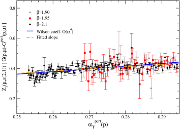
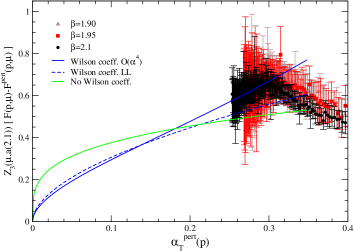
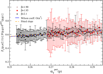
Figure 2: The left plots shows the difference between the rescaled lattice data for the gluon (top) and ghost (bottom) dressing functions and their perturbative estimate, multiplied by the square of momentum, plotted versus the perturbative Taylor coupling at the same momentum. For perturbative evaluations, $\Lambda_{\overline{\mbox{{\sc ms}}}}$ is taken to be known from $\tau$ decays. Blue dotted lines correspond to using a leading logarithm approximation for Wilson coefficient, and green solid line describes the purely perturbative ansatz. The right plots zoom into the region, from 4.5 to 6.3 GeV, where the behavior, predicted by the OPE analysis, is observed. The dotted orange line shows a linear fit of data that shows a good agreement with the predicted running.

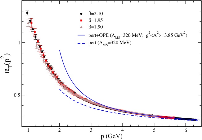
Figure 3: The Taylor coupling computed with the artefact-free lattice dressing functions and the best-fit parameters for $\Lambda_{\overline{\mbox{{\sc ms}}}}$ and $g^{2}\langle A^{2}\rangle$ (solid blue line). For the sake of comparison, the four loop perturbative prediction, evaluated for the same $\Lambda_{\overline{\mbox{{\sc ms}}}}$, is also plotted with a dashed blue line.

References

- [1] B. Alles, D. Henty, H. Panagopoulos, C. Parrinello, C. Pittori, et al. from the nonperturbatively renormalised lattice three gluon vertex. Nucl.Phys., B502:325–342, 1997.
- [2] Philippe Boucaud, J.P. Leroy, J. Micheli, O. Pène, and C. Roiesnel. Lattice calculation of alpha(s) in momentum scheme. JHEP, 9810:017, 1998.
- [3] D. Becirevic, Ph. Boucaud, J.P. Leroy, J. Micheli, O. Pene, J. Rodriguez-Quintero, and C. Roiesnel. Asymptotic behaviour of the gluon propagator from lattice QCD. Phys. Rev., D60:094509, 1999.
- [4] D. Becirevic, Ph. Boucaud, J.P. Leroy, J. Micheli, O. Pene, J. Rodriguez-Quintero, and C. Roiesnel. Asymptotic scaling of the gluon propagator on the lattice. Phys. Rev., D61:114508, 2000.
- [5] Lorenz von Smekal, Reinhard Alkofer, and Andreas Hauck. The Infrared behavior of gluon and ghost propagators in Landau gauge QCD. Phys.Rev.Lett., 79:3591–3594, 1997.
- [6] Philippe Boucaud, J.P. Leroy, A. Le Yaouanc, A.Y. Lokhov, J. Micheli, et al. Non-perturbative power corrections to ghost and gluon propagators. JHEP, 0601:037, 2006.
- [7] Philippe Boucaud, F. De Soto, J.P. Leroy, A. Le Yaouanc, J. Micheli, O. Pène, and J. Rodríguez-Quintero. Ghost-gluon running coupling, power corrections and the determination of Lambda(MS-bar). Phys.Rev., D79:014508, 2009.
- [8] Ph. Boucaud, J.P. Leroy, A. Le Yaouanc, J. Micheli, O. Pene, et al. The Infrared Behaviour of the Pure Yang-Mills Green Functions. Few Body Systems, 2012.
- [9] R. Baron, Ph. Boucaud, J. Carbonell, A. Deuzeman, V. Drach, et al. Light hadrons from lattice QCD with light (u,d), strange and charm dynamical quarks. JHEP, 1006:111, 2010.
- [10] R. Baron, B. Blossier, P. Boucaud, J. Carbonell, A. Deuzeman, et al. Light hadrons from Nf=2+1+1 dynamical twisted mass fermions. PoS, LATTICE2010:123, 2010.
- [11] Roberto Frezzotti, Pietro Antonio Grassi, Stefan Sint, and Peter Weisz. Lattice QCD with a chirally twisted mass term. JHEP, 08:058, 2001.
- [12] R. Frezzotti and G. C. Rossi. Twisted-mass lattice QCD with mass non-degenerate quarks. Nucl. Phys. Proc. Suppl., 128:193–202, 2004.
- [13] Siegfried Bethke, Andre H. Hoang, Stefan Kluth, Jochen Schieck, Iain W. Stewart, et al. Workshop on Precision Measurements of . 2011. * Temporary entry *.
- [14] K. Nakamura et al. Review of particle physics. J. Phys., G37:075021, 2010.
- [15] Mikhail A. Shifman, A.I. Vainshtein, and Valentin I. Zakharov. QCD and Resonance Physics. Sum Rules. Nucl.Phys., B147:385–447, 1979.
- [16] Mikhail A. Shifman, A.I. Vainshtein, and Valentin I. Zakharov. QCD and Resonance Physics: Applications. Nucl.Phys., B147:448–518, 1979.
- [17] B. Blossier, Ph. Boucaud, M. Brinet, F. De Soto, X. Du, et al. Ghost-gluon coupling, power corrections and from lattice QCD with a dynamical charm. Phys.Rev., D85:034503, 2012.
- [18] B. Blossier, Ph. Boucaud, M. Brinet, F. De Soto, X. Du, et al. The Strong running coupling at and mass scales from lattice QCD. Phys.Rev.Lett., 108:262002, 2012.
- [19] B. Blossier et al. Ghost-gluon coupling, power corrections and from twisted-mass lattice QCD at Nf=2. Phys. Rev., D82:034510, 2010.
- [20] Philippe Boucaud, A. Le Yaouanc, J.P. Leroy, J. Micheli, O. Pène, and J. Rodríguez-Quintero. Consistent OPE description of gluon two point and three point Green function? Phys.Lett., B493:315–324, 2000.
- [21] F. V. Gubarev and Valentin I. Zakharov. On the emerging phenomenology of ¡(A(a)(mu))**2(min)¿. Phys. Lett., B501:28–36, 2001.
- [22] Kei-Ichi Kondo. Vacuum condensate of mass dimension 2 as the origin of mass gap and quark confinement. Phys.Lett., B514:335–345, 2001.
- [23] H. Verschelde, K. Knecht, K. Van Acoleyen, and M. Vanderkelen. The Nonperturbative groundstate of QCD and the local composite operator . Phys.Lett., B516:307–313, 2001.
- [24] D. Dudal, H. Verschelde, and S.P. Sorella. The Anomalous dimension of the composite operator in the Landau gauge. Phys.Lett., B555:126–131, 2003.
- [25] Enrique Ruiz Arriola, Patrick Oswald Bowman, and Wojciech Broniowski. Landau-gauge condensates from the quark propagator on the lattice. Phys.Rev., D70:097505, 2004.
- [26] David Vercauteren and Henri Verschelde. A Two-component picture of the condensate with instantons. Phys.Lett., B697:70–74, 2011.
- [27] Philippe Boucaud, A. Le Yaouanc, J.P. Leroy, J. Micheli, O. Pène, and J. Rodríguez-Quintero. Testing Landau gauge OPE on the lattice with a gluon condensate. Phys.Rev., D63:114003, 2001.
- [28] F. De Soto and J. Rodriguez-Quintero. Notes on the determination of the Landau gauge OPE for the asymmetric three gluon vertex. Phys.Rev., D64:114003, 2001.
- [29] Philippe Boucaud, F. de Soto, J.P. Leroy, A. Le Yaouanc, J. Micheli, et al. Artefacts and power corrections: Revisiting the MOM Z psi (p**2) and Z(V). Phys.Rev., D74:034505, 2006.
- [30] B. Blossier et al. Renormalisation of quark propagators from twisted-mass lattice QCD at =2. Phys. Rev., D83:074506, 2011.
- [31] B. Blossier et al. Testing the OPE Wilson Coefficient for gluon condensate from lattice QCD with dynamical charm. Preliminary.
- [32] F. de Soto and C. Roiesnel. On the reduction of hypercubic lattice artifacts. JHEP, 0709:007, 2007.
- [33] K.G. Chetyrkin and A. Retey. Three loop three linear vertices and four loop similar to MOM beta functions in massless QCD. 2000.