Galerkin approximations for the stochastic Burgers equation

Abstract

Existence and uniqueness for semilinear stochastic evolution equations with additive noise by means of finite dimensional Galerkin approximations is established and the convergence rate of the Galerkin approximations to the solution of the stochastic evolution equation is estimated.

These abstract results are applied to several examples of stochastic partial differential equations (SPDEs) of evolutionary type including a stochastic heat equation, a stochastic reaction diffusion equation and a stochastic Burgers equation. The estimated convergence rates are illustrated by numerical simulations.

The main novelty in this article is to estimate the difference of the finite dimensional Galerkin approximations and of the solution of the infinite dimensional SPDE uniformly in space, i.e., in the $L^{\infty}$-topology, instead of the usual Hilbert space estimates in the $L^{2}$-topology, that were shown before.

1 Introduction

In this work we present a general abstract result for the spatial approximation of stochastic evolution equations with additive noise via Galerkin methods. This abstract result is applied to several examples of stochastic partial differential equations (SPDEs) of evolutionary type including a stochastic heat equation, a stochastic reaction diffusion equation and a stochastic Burgers equation. In all examples we need to verify the following conditions. First, we need the rate of approximation of the linear equation obtained by omitting the nonlinear term in the stochastic evolution equation. Then one needs a quite weak Lipschitz condition for the nonlinearity and finally a uniform bound on the sequence of approximations. These results are the key for the main theorem (see Theorem 1). The main novelty in this article is to estimate the difference of the finite dimensional Galerkin approximations and of the solution of the infinite dimensional SPDE uniformly in space, i.e., in the $L^{\infty}$-topology, instead of the usual Hilbert space estimates shown before in the $L^{2}$-topology.

Although there are several different methods using finite dimensional approximations like, for instance, spectral Galerkin, finite elements, or wavelets, we focus here on the spectral Galerkin method. Thus the finite dimensional approximations are given by an expansion in terms of the eigenfunctions of a dominant linear operator. This spectral Galerkin method is one of the key tools in the analysis of stochastic or deterministic PDEs. For SPDEs see, for example, [16, 9, 17, 2], where the Galerkin method was used to establish the existence of solutions. Moreover, spectral methods are an effective tool for numerical simulations, especially on domains, like the interval, where fast Fourier-transforms are available. Nevertheless, it is limited on domains, where the eigenfunctions of the dominant linear operator are not explicitly known. In recent years there has also been a significant interest in analytic results for the rate of approximation using a spectral Galerkin method as a numerical method for SPDEs; see, for example, [18, 28] for SPDEs with one-dimensional possibly non-additive noise and globally Lipschitz continuous nonlinearities, [31, 32, 35, 36, 25, 26] for SPDEs with possibly infinite dimensional additive noise and globally Lipschitz continuous nonlinearities, [30, 23] for SPDEs with possibly infinite dimensional additive noise and non-globally Lipschitz continuous nonlinearities, and [20, 21, 34, 33] for SPDEs with possibly infinite dimensional non-additive noise and globally Lipschitz continuous nonlinearities. In most of the above named references also the full discretization is treated including the time discretization.

In order to illustrate the main result of this article we limit ourself in this introductory section to a stochastic Burgers equation with Dirichlet boundary conditions and refer to Section 3 for the general result and to Section 4 for further examples. To this end let $T\in(0,\infty)$ be a real number, let $\left(\Omega,\mathcal{F},\mathbb{P}\right)$ be a given probability space and let $X\colon[0,T]\times\Omega\rightarrow C([0,1],\mathbb{R})$ be the up to indistinguishability unique solution process of the SPDE

$$dX_{t}(x)=\left[\frac{\partial^{2}}{\partial x^{2}}X_{t}(x)-X_{t}(x)\cdot\frac{\partial}{\partial x}X_{t}(x)\right]dt+dW_{t}(x),\;X_{t}(0)=X_{t}(1)=0,\;X_{0}=0$$ (1)

for $t\in[0,T]$ and $x\in(0,1)$, where $W_{t}$, $t\in[0,T]$, is a cylindrical $I$-Wiener process on $L^{2}((0,1),\mathbb{R})$, which models space-time white noise on $(0,1)$. In this introductory section the initial value $X_{0}=0$ is zero for simplicity of presentation and we refer to Section 4.3 below for a more general stochastic Burgers equation with a possibly non-zero initial value. The existence and uniqueness of solutions of the stochastic Burgers equation was, e.g., studied in Da Prato & Gatarek [11] for colored noise and in Da Prato, Debussche & Temam [10] for space-time white noise (see also Chapter 14 in Da Prato and Zabczyk [14]).

Recently, Alabert & Gyöngy showed the following error estimate for spatial discretizations in the $L^{2}$-topology (see Theorem 2.2 in [1]):

$$\mathbb{P}\!\left[\sup_{0\leq t\leq T}\Big{(}\int_{0}^{1}|X_{t}(x)-X_{t}^{N}(x)|^{2}\,dx\Big{)}^{1/2}\leq C_{\varepsilon}\cdot N^{\varepsilon-\frac{1}{2}}\right]=1$$ (2)

for every $N\in\mathbb{N}:=\left\{1,2,\dots\right\}$ and every arbitrarily small $\varepsilon\in(0,\frac{1}{2})$ with random variables $C_{\varepsilon}\colon\Omega\rightarrow[0,\infty)$, $\varepsilon\in(0,\frac{1}{2})$, where the $X^{N}$, $N\in\mathbb{N}$, are given by finite differences approximations. Our results (see Lemma 4, Theorem 1 and Lemma 9) yield the following estimate for the stochastic Burgers equation (1) (see Section 4.3):

$$\mathbb{P}\!\left[\sup_{0\leq t\leq T}\sup_{0\leq x\leq 1}\left|X_{t}(x)-X_{t}^{N}(x)\right|\leq C_{\varepsilon}\cdot N^{\varepsilon-\frac{1}{2}}\right]=1$$ (3)

for every $N\in\mathbb{N}$ and every arbitrarily small $\varepsilon\in(0,\frac{1}{2})$ with random variables $C_{\varepsilon}\colon\Omega\rightarrow[0,\infty)$, $\varepsilon\in(0,\frac{1}{2})$, where $X^{N}$, $N\in\mathbb{N}$, are spectral Galerkin approximations. Thus, although the spatial error criteria is estimated in the bigger $L^{\infty}$-norm instead of the $L^{2}$-norm, the convergence rate remains $\frac{1}{2}-$. This convergence rate with respect to the strong $L^{\infty}$-norm is also corroborated by a numerical example (see Section 4). (For a real number $a\in(0,\infty)$, we write $a-$ for the convergence order, if the convergence order is higher than $a-\varepsilon$ for every arbitrarily small $\varepsilon\in(0,a)$.)

A further instructive related result is given by Liu [30]. He treats stochastic reaction diffusion equations of the Ginzburg-Landau type which fit in the abstract setting in Section 2. For such equations he obtained estimates in the $H^{r}$-topology with the rate $(\frac{1}{2}-r)-$ for every $r\in(0,\frac{1}{2})$. The convergence rates he obtained in the $H^{r}$-topologoy with $r\in(0,\frac{1}{2})$ can, in general, not be improved and, by using Sobolev embeddings, his bounds also yield estimates in the $L^{p}$-topology with $p\in(2,\infty)$. Nevertheless, such estimates do not yield convergence in the $L^{\infty}$-topology, since in one dimension $H^{r}$ is embedded into $L^{\infty}$ for $r>\frac{1}{2}$ only. Moreover, in contrast to (3) this would not give a convergence rate $\frac{1}{2}-$ in any $L^{p}$-topology where $p\in(2,\infty]$.

The rest of the paper is organized as follows. Section 2 gives the setting and the assumptions for the main result, which is then presented in Section 3. In Section 4 we discuss our examples, while in the final section most of the proofs are stated.

Next we add that after the preprint version [3] of this article has appeared, a number of related results appeared in the literature; see, e.g., [6, 19, 29, 8, 7, 15, 4]. In particular, we mention [8, 7] for temporal and spatial discretization estimates in Banach spaces that imply estimates in the $L^{\infty}$-norm as well as [29] for the analysis of spectral Galerkin methods for semilinear SPDEs with possibly non-additive noise and globally Lipschitz continuous nonlinearities. We also refer, e.g., to [19] for further spatial approximations of stochastic Burgers equations and, e.g., to [6, 15] for the analysis of spatial and temporal-spatial discretizations of stochastic Navier-Stokes equations. Finally, we would like to point out that parts of this article (see Subsection 4.1) appeared in the thesis [24] (see Section 2.2.3 in [24]).

2 Setting and assumptions

Throughout this article suppose that the following setting and the following assumptions are fulfilled.

The first assumption is a regularity and approximation condition on the semigroup of the linear operator of the considered SPDE. The second is an appropriate Lipschitz condition on the nonlinearity of the considered SPDE. The third is an assumption on the approximation of the stochastic convolution and the initial value of the considered SPDE while the final one is a uniform bound on finite dimensional approximations of the considered SPDE.

Let $T\in(0,\infty)$, let $(\Omega,\mathcal{F},\mathbb{P})$ be a probability space and let $(V,\left\|\cdot\right\|_{V})$ and $(W,\left\|\cdot\right\|_{W})$ be two $\mathbb{R}$-Banach spaces. Moreover, let $P_{N}\colon V\rightarrow V$, $N\in\mathbb{N}$, be a sequence of bounded linear operators from $V$ to $V$.

Assumption 1 (Semigroup $S$).

Let $\alpha\in[0,1)$ and $\gamma\in(0,\infty)$ be real numbers and let $S\colon(0,T]\rightarrow L(W,V)$ be a strongly continuous mapping which satisfies $\sup_{t\in(0,T]}\left(t^{\alpha}\left\|S_{t}\right\|_{L(W,V)}\right)<\infty$ and $\sup_{N\in\mathbb{N}}\sup_{t\in(0,T]}\left(t^{\alpha}N^{\gamma}\left\|S_{t}-P_{N}S_{t}\right\|_{L(W,V)}\right)<\infty$.

Assumption 2 (Nonlinearity $F$).

Let $F\colon V\rightarrow W$ be a mapping which satisfies $\sup_{\begin{subarray}{c}\|v\|_{V},\|w\|_{V}\leq r,\,v\neq w\end{subarray}}\frac{\left\|F(v)-F(w)\right\|_{W}}{\left\|v-w\right\|_{V}}<\infty$ for every $r\in(0,\infty)$.

Assumption 3 (Stochastic process $O$).

Let $O\colon[0,T]\times\Omega\rightarrow V$ be a stochastic process with continuous sample paths and $\sup_{N\in\mathbb{N}}\sup_{0\leq t\leq T}N^{\gamma}\left\|O_{t}(\omega)-P_{N}(O_{t}(\omega))\right\|_{V}<\infty$ for every $\omega\in\Omega$, where $\gamma\in(0,\infty)$ is given in Assumption 1.

Assumption 4 (Existence of solutions).

Let $X^{N}\colon[0,T]\times\Omega\rightarrow V$, $N\in\mathbb{N}$, be a sequence of stochastic processes with continuous sample paths and with

$$X^{N}_{t}(\omega)=\int^{t}_{0}P_{N}\,S_{t-s}\,F(X^{N}_{s}(\omega))\,ds+P_{N}(O_{t}(\omega))\quad\text{and}\quad\sup_{M\in\mathbb{N}}\sup_{s\in[0,T]}\|X^{M}_{s}(\omega)\|_{V}<\infty$$ (4)

for every $t\in[0,T]$, $\omega\in\Omega$ and every $N\in\mathbb{N}$.

As usual, we call here a mapping $Y\colon[0,T]\times\Omega\rightarrow V$ a stochastic process, if for every $t\in[0,T]$ the mapping $Y_{t}\colon\Omega\ni\omega\mapsto Y_{t}(\omega):=Y(t,\omega)\in V$ is $\mathcal{F}$/$\mathcal{B}(V)$-measurable. Additionally, we say that a stochastic process $Y\colon[0,T]\times\Omega\rightarrow V$ has continuous sample paths, if for every $\omega\in\Omega$ the mapping $[0,T]\ni t\mapsto Y_{t}(\omega)\in V$ is continuous. Furthermore, we say that a mapping $f\colon(0,T]\to L(W,V)$ is strongly continuous if for every $w\in W$ the mapping $(0,T]\ni t\mapsto f(t)w\in V$ is continuous. Moreover, note that if $Y\colon[0,T]\times\Omega\rightarrow V$ is a stochastic process with continuous sample paths, then Assumptions 1 and 2 ensure for every $\omega\in\Omega$, $t\in(0,T]$ and every $N\in\mathbb{N}$ that the mapping $(0,t)\ni s\mapsto P_{N}\,S_{t-s}\,F(Y_{s}(\omega))\in V$ is continuous and therefore, we obtain for every $\omega\in\Omega$, $t\in[0,T]$ and every $N\in\mathbb{N}$ that the $V$-valued Bochner integral $\int^{t}_{0}P_{N}\,S_{t-s}\,F(Y_{s}(\omega))\,ds\in V$ (see (4) in Assumption 4) is well defined.

3 Main result

In this section we state the main approximation result, which is based on the assumptions of the previous section. Its proof is postponed to Subsection 5.1.

Theorem 1.

Let Assumptions 1-4 be fulfilled. Then there exists a unique stochastic process $X\colon[0,T]\times\Omega\rightarrow V$ with continuous sample paths which fulfills

$$X_{t}(\omega)=\int^{t}_{0}S_{t-s}\,F(X_{s}(\omega))\,ds+O_{t}(\omega)$$ (5)

for every $t\in[0,T]$ and every $\omega\in\Omega$. Moreover, there exists an $\mathcal{F}$/$\mathcal{B}([0,\infty))$-measurable mapping $C\colon\Omega\rightarrow[0,\infty)$ such that

$$\sup_{0\leq t\leq T}\left\|X_{t}(\omega)-X^{N}_{t}(\omega)\right\|_{V}\leq C(\omega)\cdot N^{-\gamma}$$ (6)

for every $N\in\mathbb{N}$ and every $\omega\in\Omega$ where $\gamma\in(0,\infty)$ is given in Assumption 1.

Let us add three remarks on Theorem 1. First, we would like to point out that the initial value of the stochastic evolution equation (5) is incorporated in the driving stochastic process $O\colon[0,T]\times\Omega\rightarrow V$ (see also Proposition 3 below for more details). Second, we emphasize that the driving stochastic processes $O\colon[0,T]\times\Omega\rightarrow V$ is not assumed to be a stochastic convolution of the semigroup and a cylindrical Wiener process. In particular, the stochastic evolution equation (5) covers SPDEs disturbed by fractional Brownian motions too. Third, we would like to point out that Theorem 1 yields the existence of an $\mathcal{F}$/$\mathcal{B}([0,\infty))$-measurable mapping $C\colon\Omega\rightarrow[0,\infty)$ such that (6) holds although the $\mathbb{R}$-Banach space $\left(V,\left\|\cdot\right\|_{V}\right)$ is not assumed to be separable. The sum and the difference of two $\mathcal{F}$/$\mathcal{B}(V)$-measurable mappings on the possibly non-separable $\mathbb{R}$-Banach space $V$ are, in general, not $\mathcal{F}$/$\mathcal{B}(V)$-measurable anymore. Nonetheless, it is possible to establish the existence of an $\mathcal{F}$/$\mathcal{B}([0,\infty))$-measurable mapping $C\colon\Omega\rightarrow[0,\infty)$ such that (6) holds by exploiting for every $t\in[0,T]$ and every $N\in\mathbb{N}$ that the difference $O_{t}-P_{N}(O_{t})=(I-P_{N})\,O_{t}\colon\Omega\to V$ is $\mathcal{F}$/$\mathcal{B}(V)$-measurable (see (27) in the proof of Theorem 1 for more details). Note that the composition of two measurable mappings is measurable (on non-separable $\mathbb{R}$-Banach spaces too). Finally, we note that the error constant $C\colon\Omega\rightarrow[0,\infty)$ appearing in (6) is described explicitly in the proof of Theorem 1 (see definition (33) in the proof of Theorem 1 for details).

4 Examples

This section presents some examples of the setting in Section 2.

4.1 Stochastic heat equation

In this subsection an important example of Assumption 3 is presented. We consider a linear equation with $F=0$ and thus consider only the approximation of the Ornstein-Uhlenbeck process $O$.

To this end let $d\in\mathbb{N}$ and let $V=W=C([0,1]^{d},\mathbb{R})$ be the $\mathbb{R}$-Banach space of continuous functions from $[0,1]^{d}$ to $\mathbb{R}$ equipped with the supremum norm $\left\|\cdot\right\|_{V}=\left\|\cdot\right\|_{W}=\left\|\cdot\right\|_{C([0,1]^{d},\mathbb{R})}$. Moreover, consider the continuous functions $e_{i}\colon[0,1]^{d}\rightarrow\mathbb{R}$, $i\in\mathbb{N}^{d}$, and the real numbers $\lambda_{i}$, $i\in\mathbb{N}^{d}$, defined through

$$e_{i}(x):=2^{\frac{d}{2}}\sin(i_{1}\pi x_{1})\ldots\sin(i_{d}\pi x_{d})\qquad\text{and}\qquad\lambda_{i}:=\pi^{2}\big{(}|i_{1}|^{2}+\ldots+|i_{d}|^{2}\big{)}$$ (7)

for all $x=(x_{1},\dots,x_{d})\in[0,1]^{d}$ and all $i=(i_{1},\dots,i_{d})\in\mathbb{N}^{d}$. Additionally, suppose that the bounded linear operators $P_{N}\colon C([0,1]^{d},\mathbb{R})\rightarrow C([0,1]^{d},\mathbb{R})$, $N\in\mathbb{N}$, are given by

$$(P_{N}(v))(x)=\sum_{i\in\{1,\dots,N\}^{d}}\int_{(0,1)^{d}}e_{i}(s)\,v(s)\,ds\cdot e_{i}(x)$$ (8)

for all $x\in[0,1]^{d}$, $v\in C([0,1]^{d},\mathbb{R})$ and all $N\in\mathbb{N}$. The linear operators $P_{N}$, $N\in\mathbb{N}$, are projection operators, i.e., they satisfy $P_{N}(P_{N}(v))=P_{N}(v)$ for all $v\in C([0,1]^{d},\mathbb{R})$ and all $N\in\mathbb{N}$ and their images are the finite dimensional $\mathbb{R}$-vector spaces $P_{N}\big{(}C([0,1]^{d},\mathbb{R})\big{)}$, $N\in\mathbb{N}$. The operators $P_{N}$, $N\in\mathbb{N}$, are thus compact linear operators and from the Daugavet property of the $\mathbb{R}$-Banach space $C([0,1]^{d},\mathbb{R})$ (see, e.g., Definition 2.1 and Example (a) in Werner [40]) we get that $\|I-P_{N}\|_{L(C([0,1]^{d},\mathbb{R}))}=1+\|P_{N}\|_{L(C([0,1]^{d},\mathbb{R}))}$ for all $N\in\mathbb{N}$ (see, for instance, Theorem 2.7 in Werner [40]). Next let $S\colon(0,T]\rightarrow L(C([0,1]^{d},\mathbb{R}))$ be a mapping given by

$$(S_{t}v)(x)=\sum_{i\in\mathbb{N}^{d}}e^{-\lambda_{i}t}\int_{(0,1)^{d}}e_{i}(s)\,v(s)\,ds\cdot e_{i}(x)$$ (9)

for all $t\in(0,T]$, $x\in[0,1]^{d}$ and all $v\in C([0,1]^{d},\mathbb{R})$.

Lemma 2.

Let $d\in\left\{1,2,3\right\}$. Then the mapping $S\colon(0,T]\rightarrow L(C([0,1]^{d},\mathbb{R}))$ given by (9) satisfies Assumption 1 for every $\alpha\in[\frac{d}{4}+\frac{\gamma}{2},1)$ and every $\gamma\in(0,2-\frac{d}{2})$.

Clearly, this is simply the semigroup generated by the Laplacian with Dirichlet boundary conditions (see, e.g., Section 3.8.1 in [39]). Other boundary conditions such as Neumann or periodic boundary conditions could also be considered here. The proof of Lemma 2 is well-known and therefore omitted. We also add that the proof of Lemma 2 essentially uses a suitable Sobolev embedding and for this the condition $d\leq 3$ is assumed in Lemma 2. We now present the promised example of Assumption 3. We consider a stochastic convolution of the semigroup $S$ constructed in (9) and a cylindrical Wiener process. The following result provides an appropriate version of such a process, in which the initial value of the stochastic evolution equation (5) is additionally incorporated.

Proposition 3.

Let $d\in\mathbb{N}$, let $V=C([0,1]^{d},\mathbb{R})$ with $\|v\|_{V}=\|v\|_{C([0,1]^{d},\mathbb{R})}$ for every $v\in V$, let $\rho\in(0,\infty)$, let $\beta^{i}\colon[0,T]\times\Omega\rightarrow\mathbb{R}$, $i\in\mathbb{N}^{d}$, be a family of independent standard Brownian motions with continuous sample paths and let $b\colon\mathbb{N}^{d}\rightarrow\mathbb{R}$ be a function with $\sum_{i\in\mathbb{N}^{d}}\left(i_{1}^{2}+\ldots+i_{d}^{2}\right)^{\left(\rho-1\right)}|b(i)|^{2}<\infty$. Furthermore, suppose that $\xi\colon\Omega\rightarrow V$ is an $\mathcal{F}$/$\mathcal{B}(V)$-measurable mapping with $\sup_{N\in\mathbb{N}}\left(N^{\rho}\left\|\xi(\omega)-P_{N}(\xi(\omega))\right\|_{V}\right)<\infty$ for every $\omega\in\Omega$. Then there exists an up to indistinguishability unique stochastic process $O\colon[0,T]\times\Omega\rightarrow V$ with continuous sample paths which satisfies

$$\mathbb{P}\bigg{[}\lim_{N\rightarrow\infty}\,\sup_{0<t\leq T}\Big{\|}O_{t}-S_{t}\,\xi-\!\!\!\!\!\!\sum_{i\in\{1,\dots,N\}^{d}}\!\!\!\!\!\!b(i)\,\Big{(}-\lambda_{i}\int^{t}_{0}e^{-\lambda_{i}(t-s)}\beta^{i}_{s}\,ds+\beta^{i}_{t}\Big{)}\,e_{i}\Big{\|}_{V}=0\bigg{]}=1$$ (10)

and

$$\sup_{N\in\mathbb{N}}\sup_{0\leq t\leq T}\big{(}N^{\gamma}\|O_{t}(\omega)-P_{N}(O_{t}(\omega))\|_{V}\big{)}<\infty$$ (11)

for every $\omega\in\Omega$ and every $\gamma\in(0,\rho)$. In particular, $O$ satisfies Assumption 3 for every $\gamma\in(0,\rho)$. Here the functions $e_{i}\in V$, $i\in\mathbb{N}^{d}$, the real numbers $\lambda_{i}$, $i\in\mathbb{N}^{d}$, and the linear operators $P_{N}\colon V\rightarrow V$, $N\in\mathbb{N}$, are given in (7) and (8).

Proposition 3 follows directly from Lemma 4 below. Let us add some remarks concerning Proposition 3. Let $L^{2}((0,1)^{d},\mathbb{R})$ be the $\mathbb{R}$-Hilbert space of equivalence classes of $\mathcal{B}((0,1)^{d})$/$\mathcal{B}(\mathbb{R})$-measurable and Lebesgue square integral functions from $(0,1)^{d}$ to $\mathbb{R}$ and let $B\colon L^{2}((0,1)^{d},\mathbb{R})\rightarrow L^{2}((0,1)^{d},\mathbb{R})$ be a bounded linear operator given by

$$Bv=\sum_{i\in\mathbb{N}^{d}}b(i)\int_{(0,1)^{d}}e_{i}(s)\,v(s)\,ds\cdot e_{i}$$ (12)

for all $v\in L^{2}((0,1)^{d},\mathbb{R})$ where $b\colon\mathbb{N}^{d}\rightarrow\mathbb{R}$ is the function used in Proposition 3. Then the stochastic process $O\colon[0,T]\times\Omega\rightarrow C([0,1]^{d},\mathbb{R})$ in Proposition 3 satisfies

$$\begin{split}O_{t}&=S_{t}\,\xi+\sum_{i\in\mathbb{N}^{d}}b(i)\int^{t}_{0}e^{-\lambda_{i}(t-s)}\,d\beta^{i}_{s}\cdot e_{i}=S_{t}\,\xi+\int_{0}^{t}S_{t-s}\,B\,dW_{s}\end{split}$$ (13)

$\mathbb{P}$-a.s. for every $t\in(0,T]$ where $W_{t}$, $t\in[0,T]$, is an appropriate cylindrical $I$-Wiener process on $L^{2}((0,1)^{d},\mathbb{R})$. In particular, $O\colon[0,T]\times\Omega\rightarrow C([0,1]^{d},\mathbb{R})$ is the up to indistinguishability unique mild solution process of the linear SPDE

$$dO_{t}=\big{[}\Delta O_{t}\big{]}\,dt+B\,dW_{t},\qquad O_{t}|_{\partial(0,1)^{d}}\equiv 0,\qquad O_{0}=\xi$$ (14)

for $t\in[0,T]$ on $C([0,1]^{d},\mathbb{R})$. The process $O$ thus includes the initial value and a stochastic convolution of the semigroup generated by the Laplacian with Dirichlet boundary conditions and a cylindrical Wiener process as it is frequently considered in the literature (see, e.g., Section 5 in [13]). Note also that the operator $B$ appearing in (14) is diagonal with respect to the orthonormal basis $e_{i}\in L^{2}((0,1)^{d},\mathbb{R})$, $i\in\mathbb{N}^{d}$, in $L^{2}((0,1)^{d},\mathbb{R})$. This assumption is strongly exploited in Proposition 3. However, the abstract setting in Section 2 does not need this assumption to be fulfilled and, in principle, linear operators $B$ that are not diagonal with respect to $e_{i}$, $i\in\mathbb{N}^{d}$, could be considered here. The detailed analysis in the non-diagonal case remains an open question for future research. The reader is referred to [4] for first results in that direction.

To illustrate Proposition 3 we consider the following simple example. If $d=2$, $(\xi(\omega))(x)=0$ for all $x\in[0,1]^{2}$, $\omega\in\Omega$ and $b((i_{1},i_{2}))=\frac{1}{(i_{1}+i_{2})}$ for all $i=(i_{1},i_{2})\in\mathbb{N}^{2}$ in Proposition 3, then Proposition 3 implies the existence of $\mathcal{F}$/$\mathcal{B}([0,\infty))$-measurable mappings $C_{\gamma}\colon\Omega\rightarrow[0,\infty)$, $\gamma\in(0,1)$, such that

$$\sup_{0\leq t\leq 1}\sup_{x\in[0,1]^{2}}\big{|}O_{t}(\omega,x)-(P_{N}O_{t})(\omega,x)\big{|}\leq C_{\gamma}(\omega)\cdot N^{-\gamma}$$ (15)

for all $\omega\in\Omega$, $N\in\mathbb{N}$ and all $\gamma\in(0,1)$. Finally, note that Proposition 3 follows immediately from the next result (Lemma 4), which is also of independent interest. Its proof is postponed to Subsection 5.2.1. Estimates related to Lemma 4 and its proof can, e.g., be found in Section 5.5.1 in Da Prato & Zabczyk [13] and in Proposition 1.1 and Proposition 1.2 in Da Prato & Debussche [9]. In particular, the temporal regularity statements in Lemma 4 follow, e.g., immediately from Lemma 5.19 and Theorem 5.20 in [13].

Lemma 4.

Let $d\in\mathbb{N}$, let $V=C([0,1]^{d},\mathbb{R})$ with $\|v\|_{V}=\|v\|_{C([0,1]^{d},\mathbb{R})}$ for every $v\in V$, let $\rho\in(0,\infty)$, let $\beta^{i}\colon[0,T]\times\Omega\rightarrow\mathbb{R}$, $i\in\mathbb{N}^{d}$, be a family of independent standard Brownian motions with continuous sample paths and let $b\colon\mathbb{N}^{d}\rightarrow\mathbb{R}$ be a function with $\sum_{i\in\mathbb{N}^{d}}\left(i_{1}^{2}+\ldots+i_{d}^{2}\right)^{\left(\rho-1\right)}|b(i)|^{2}<\infty$. Then there exists an up to indistinguishability unique stochastic process $O\colon[0,T]\times\Omega\rightarrow V$ which satisfies

$$\sup_{N\in\mathbb{N}}\sup_{0\leq t\leq T}\!\big{(}N^{\gamma}\left\|O_{t}(\omega)-P_{N}(O_{t}(\omega))\right\|_{V}\!\big{)}+\sup_{0\leq t_{1}<t_{2}\leq T}\frac{\left\|O_{t_{2}}(\omega)-O_{t_{1}}(\omega)\right\|_{V}}{\left|t_{2}-t_{1}\right|^{\theta}}<\infty$$

for every $\omega\in\Omega$, every $\theta\in(0,\min(\frac{1}{2},\frac{\rho}{2}))$, every $\gamma\in(0,\rho)$ and which satisfies

$$\sup_{N\in\mathbb{N}}\Big{\{}N^{\gamma}\Big{(}\mathbb{E}\Big{[}\sup_{0\leq t\leq T}\|O_{t}-P_{N}(O_{t})\|_{V}^{p}\Big{]}\Big{)}^{\!\frac{1}{p}}\Big{\}}+\sup_{0\leq t_{1}<t_{2}\leq T}\!\!\frac{\left(\mathbb{E}\!\left[\|O_{t_{2}}-O_{t_{1}}\|_{V}^{p}\right]\right)^{\frac{1}{p}}}{\left|t_{2}-t_{1}\right|^{\theta}}<\infty$$

and

$$\mathbb{P}\!\left[\lim_{N\rightarrow\infty}\,\sup_{0\leq t\leq T}\Big{\|}O_{t}-\sum_{i\in\left\{1,\dots,N\right\}^{d}}b(i)\Big{(}-\lambda_{i}\int^{t}_{0}e^{-\lambda_{i}(t-s)}\beta^{i}_{s}\,ds+\beta^{i}_{t}\Big{)}\cdot e_{i}\Big{\|}_{V}=0\right]=1$$

for every $p\in[1,\infty)$, every $\theta\in(0,\frac{\rho}{2})\cap[0,\frac{1}{2}]$ and every $\gamma\in(0,\rho)$. Here the functions $e_{i}\in V$, $i\in\mathbb{N}^{d}$, the real numbers $\lambda_{i}$, $i\in\mathbb{N}^{d}$, and the linear operators $P_{N}\colon V\rightarrow V$, $N\in\mathbb{N}$, are given in (7) and (8).

4.2 Stochastic evolution equations with a globally Lipschitz nonlinearity

If the nonlinearity $F\colon V\rightarrow W$ given in Assumption 2 is globally Lipschitz continuous from $V$ to $W$, then Assumption 4 is naturally met.

Proposition 5.

Suppose that Assumptions 1-3 are fulfilled. If the nonlinearity $F\colon V\rightarrow W$ given in Assumption 2 additionally satisfies $\sup_{v,w\in V,v\neq w}\frac{\|F(v)-F(w)\|_{W}}{\|v-w\|_{V}}<\infty,$ then Assumption 4 is fulfilled.

The proof of Proposition 5 is straightforward and therefore omitted. In the remainder of this section we illustrate Theorem 1 with a stochastic reaction diffusion equation with a globally Lipschitz nonlinearity. The next lemma describes the nonlinearities considered in this subsection. Its proof is clear and hence omitted.

Lemma 6.

Let $d\in\mathbb{N}$ and let $f\colon[0,1]^{d}\times\mathbb{R}\rightarrow\mathbb{R}$ be a continuous function which satisfies

$$\sup_{x\in[0,1]^{d}}\sup_{\begin{subarray}{c}y_{1},y_{2}\in\mathbb{R}\\ y_{1}\neq y_{2}\end{subarray}}\frac{|f(x,y_{1})-f(x,y_{2})|}{|y_{1}-y_{2}|}<\infty.$$ (16)

Then the corresponding Nemytskii operator $F\colon C([0,1]^{d},\mathbb{R})\rightarrow C([0,1]^{d},\mathbb{R})$ given by $(F(v))(x)=f(x,v(x))$ for every $x\in[0,1]^{d}$ and every $v\in C([0,1]^{d},\mathbb{R})$ satisfies

$$\sup_{v,w\in V,v\neq w}\frac{\|F(v)-F(w)\|_{C([0,1]^{d},\mathbb{R})}}{\|v-w\|_{C([0,1]^{d},\mathbb{R})}}<\infty.$$ (17)

Let $d\in\{1,2,3\}$ and $V=W=C([0,1]^{d},\mathbb{R})$ and let $P_{N}\colon V\rightarrow V$, $N\in\mathbb{N}$, $S\colon(0,T]\rightarrow L(V)$, $F\colon V\rightarrow V$ and $O\colon[0,T]\times\Omega\rightarrow V$ be given by (8), by (9), by Lemma 6 and by Proposition 3. Then Assumption 4 is fulfilled due to Proposition 5 and therefore, the assumptions in Theorem 1 are fulfilled. In addition, the stochastic evolution equation (5) reduces in this case to

$$dX_{t}=\big{[}\Delta X_{t}+f(\cdot,X_{t})\big{]}\,dt+B\,dW_{t},\qquad X_{t}|_{\partial(0,1)^{d}}\equiv 0,\qquad X_{0}=\xi$$ (18)

for $t\in[0,T]$, where $W_{t}$, $t\in[0,T]$, is a cylindrical $I$-Wiener process on $L^{2}((0,1)^{d},\mathbb{R})$, where $\xi\colon\Omega\rightarrow V$ is used in Proposition 3 and where the bounded linear operator $B\colon L^{2}((0,1)^{d},\mathbb{R})$ $\rightarrow$ $L^{2}((0,1)^{d},\mathbb{R})$ is given by (12) with $b\colon\mathbb{N}^{d}\rightarrow\mathbb{R}$ used in Proposition 3. Moreover, the finite dimensional SODEs (4) reduce to

$$dX^{N}_{t}=\left[\Delta X^{N}_{t}+P_{N}f(\cdot,X^{N}_{t})\right]dt+P_{N}B\,dW_{t},\quad X^{N}_{t}|_{\partial(0,1)^{d}}\equiv 0,\quad X_{0}^{N}=P_{N}(\xi)$$

for $t\in[0,T]$ and $N\in\mathbb{N}$. If $d=1$ and $b(i)=b(1)$ for all $i\in\mathbb{N}$, then Lemma 2, Proposition 3 and Theorem 1 yield the existence of $\mathcal{F}$/$\mathcal{B}([0,\infty))$-measurable mappings $C_{\gamma}\colon\Omega\rightarrow[0,\infty)$, $\gamma\in(0,\frac{1}{2})$, such that

$$\sup_{0\leq t\leq T}\sup_{0\leq x\leq 1}\big{|}X_{t}(\omega,x)-X^{N}_{t}(\omega,x)\big{|}\leq C_{\gamma}(\omega)\cdot N^{-\gamma}$$ (19)

for every $\omega\in\Omega$, $N\in\mathbb{N}$ and every $\gamma\in(0,\frac{1}{2})$. Hence, in the case $d=1$ and $b(i)=b(1)$ for all $i\in\mathbb{N}$, we obtain that $X^{N}_{t}(\omega,x)$ converges to $X_{t}(\omega,x)$ uniformly in $t\in[0,T]$ and $x\in[0,1]$ with the rate $\frac{1}{2}-$ as $N$ goes to infinity for every $\omega\in\Omega$.

4.3 Stochastic Burgers equation

In this subsection a stochastic Burgers equation is formulated in the setting of Section 2. For this a few function spaces from the literature (see, e.g., Chapter 5 in [37]) are presented first. By $(L^{2}((0,1),\mathbb{R}),$ $\left\|\cdot\right\|_{L^{2}},$ $\left<\cdot,\cdot\right>_{L^{2}})$ the $\mathbb{R}$-Hilbert space of equivalence classes of $\mathcal{B}(0,1)$/$\mathcal{B}(\mathbb{R})$-measurable and Lebesgue square integrable functions from $(0,1)$ to $\mathbb{R}$ with scalar product $\left<v,w\right>_{L^{2}}:=\int^{1}_{0}v(x)\,w(x)\,dx$ and norm $\|v\|_{L^{2}}:=(\left<v,v\right>_{L^{2}})^{1/2}$ for every $v,w\in L^{2}((0,1),\mathbb{R})$ is denoted. In addition, by $H^{1}((0,1),\mathbb{R})$ the Sobolev space of weakly differentiable functions from $(0,1)$ to $\mathbb{R}$ with weak derivatives in $L^{2}((0,1),\mathbb{R})$ is denoted. The norm and the scalar product in $H^{1}((0,1),\mathbb{R})$ are defined by $\|v\|_{H^{1}}:=(\|v\|_{L^{2}}^{2}+\|v^{\prime}\|_{L^{2}}^{2})^{1/2}$ and $\left<v,w\right>_{H^{1}}:=\left<v,w\right>_{L^{2}}+\left<v^{\prime},w^{\prime}\right>_{L^{2}}$ for every $v,w\in H^{1}((0,1),\mathbb{R})$. Additionally, by $H^{1}_{0}((0,1),\mathbb{R})$ the closure of $C^{\infty}_{\mathrm{cpt}}((0,1),\mathbb{R})$ in the $\mathbb{R}$-Hilbert space $($ $H^{1}((0,1),\mathbb{R}),$ $\left\|\cdot\right\|_{H^{1}},$ $\left<\cdot,\cdot\right>_{H^{1}})$ is denoted and the norm and the scalar product in $H^{1}_{0}((0,1),\mathbb{R})$ are denoted by $\|v\|_{H^{1}_{0}}:=\|v^{\prime}\|_{L^{2}}$ and $\left<v,w\right>_{H^{1}_{0}}:=\left<v^{\prime},w^{\prime}\right>_{L^{2}}$ for every $v,w\in H^{1}_{0}((0,1),\mathbb{R})$. The Sobolev space $(H^{-1}((0,1),\mathbb{R}),\left\|\cdot\right\|_{H^{-1}})$ $:=$ $(H^{1}_{0}((0,1),\mathbb{R}),\left\|\cdot\right\|_{H^{1}_{0}})^{\prime}$ is also used below and by $\partial\colon L^{2}((0,1),\mathbb{R})\rightarrow H^{-1}((0,1),\mathbb{R})$ the distributional derivative in $L^{2}((0,1),\mathbb{R})$ defined by $(\partial v)(\varphi)=(v^{\prime})(\varphi):=-\left<v,\varphi^{\prime}\right>_{L^{2}}$ for every $\varphi\in H^{1}_{0}((0,1),\mathbb{R})$ and every $v\in L^{2}((0,1),\mathbb{R})$ is denoted.

In view of these function spaces, let $W=H^{-1}((0,1),\mathbb{R})$ with $\|v\|_{W}:=\|v\|_{H^{-1}}$ for all $v\in W$ and let $V=C([0,1],\mathbb{R})$ with $\|v\|_{V}:=\sup_{x\in[0,1]}|v(x)|$ for all $v\in V$ be the $\mathbb{R}$-Banach space of continuous functions from $[0,1]$ to $\mathbb{R}$. As in Sections 4.1 and 4.2, we use the projection operators $P_{N}\colon C([0,1],\mathbb{R})\rightarrow C([0,1],\mathbb{R})$, $N\in\mathbb{N}$, defined by

$$\big{(}P_{N}(v)\big{)}(x):=\sum^{N}_{n=1}2\int^{1}_{0}\sin(n\pi s)\,v(s)\,ds\cdot\sin(n\pi x)$$ (20)

for every $x\in[0,1]$, $v\in C([0,1],\mathbb{R})$ and every $N\in\mathbb{N}$. The semigroup is constructed in the following well-known lemma here.

Lemma 7.

The mapping $S\colon(0,T]\rightarrow L\big{(}H^{-1}((0,1),\mathbb{R}),C([0,1],\mathbb{R})\big{)}$ given by $\big{(}S_{t}(w)\big{)}(x)=\sum^{\infty}_{n=1}2\cdot e^{-n^{2}\pi^{2}t}\cdot w(\sin(n\pi(\cdot)))\cdot\sin(n\pi x)$ for every $x\in[0,1]$, $w\in H^{-1}((0,1),\mathbb{R})$ and every $t\in(0,T]$ is well defined and satisfies Assumption 1 for every $\gamma\in(0,\frac{1}{2})$.

The proof of Lemma 7 can be found in Subsection 5.3.1. The next well-known lemma describes the nonlinearities for the stochastic Burgers equations considered in this section.

Lemma 8.

Let $c\in\mathbb{R}$ be a real number. Then the mapping $F\colon C([0,1],\mathbb{R})\rightarrow H^{-1}((0,1),\mathbb{R})$ given by $F(v)=c\cdot\partial\big{(}v^{2}\big{)}$ for every $v\in C([0,1],\mathbb{R})$ satisfies Assumption 2.

Proof.

The estimate $\left\|\partial v\right\|_{H^{-1}}\leq\left\|v\right\|_{L^{2}}$ for every $v\in L^{2}((0,1),\mathbb{R})$ implies

$$\begin{split}&\|F(v)-F(w)\|_{H^{-1}}=\|c\,\partial(v^{2})-c\,\partial(w^{2})\|_{H^{-1}}\leq|c|\cdot\|v^{2}-w^{2}\|_{L^{2}}\\ &\leq|c|\cdot(\|v\|_{C([0,1],\mathbb{R})}+\|w\|_{C([0,1],\mathbb{R})})\cdot\|v-w\|_{C([0,1],\mathbb{R})}\end{split}$$ (21)

for every $v,w\in C([0,1],\mathbb{R})$. This yields $\left\|F(v)-F(w)\right\|_{H^{-1}}\leq 2\,r\,|c|\left\|v-w\right\|_{C([0,1],\mathbb{R})}$ for every $v,w\in C([0,1],\mathbb{R})$ with $\|v\|_{C([0,1],\mathbb{R})},\|w\|_{C([0,1],\mathbb{R})}\leq r$ and every $r\in(0,\infty)$. The proof of Lemma 8 is thus completed. ∎

For this type of nonlinearities, Assumption 4 is fulfilled, which can be seen in the following lemma. Its proof is postponed to Subsection 5.3.2 below. A related result with can be found in Da Prato, Debussche & Temam [10] (see Lemma 3.1 and Theorem 3.1 in [10]).

Lemma 9.

Let $V=C([0,1],\mathbb{R})$ with $\|v\|_{V}=\sup_{0\leq x\leq 1}|v(x)|$ for all $v\in V$, let $W=H^{-1}((0,1),\mathbb{R})$ with $\|v\|_{W}=\|v\|_{H^{-1}}$ for all $v\in W$ and let $S\colon(0,T]\rightarrow L(W,V)$, $F\colon V\rightarrow W$ and $P_{N}\colon V\rightarrow V$, $N\in\mathbb{N}$, be given by Lemma 7, Lemma 8 and (20). Moreover, let $O\colon[0,T]\times\Omega\rightarrow V$ be an arbitrary stochastic process with continuous sample paths and with $\sup_{N\in\mathbb{N}}\sup_{0\leq t\leq T}\left\|P_{N}(O_{t}(\omega))\right\|_{V}<\infty$ for every $\omega\in\Omega$. Then Assumption 4 is fulfilled.

We emphasize that Lemma 9 does not assume that the driving noise process $O\colon[0,T]\times\Omega\rightarrow V$ is a stochastic convolution involving a cylindrical Wiener process as considered in Proposition 3. In particular, Lemma 9 covers stochastic Burgers equations driven by fractional Brownian motions. In the next step the consequences of Lemmas 7–9 and Theorem 1 are illustrated by a numerical example.

Numerical Example

We consider the stochastic evolution equation (5) with $S\colon(0,T]\rightarrow L(W,V)$, $F\colon V\rightarrow W$ and $O\colon[0,T]\times\Omega\rightarrow V$ given by Lemma 7, Lemma 8 and Proposition 3 with the parameters $c=-30$, $T=\frac{1}{20}$, $\xi(\omega)=\frac{6}{5}\sin(\pi x)$ for every $\omega\in\Omega$ and $b(i)=\frac{1}{3}$ for every $i\in\mathbb{N}$. The stochastic evolution equation (5) then reduces to

$$dX_{t}(x)=\Big{[}\Delta X_{t}-60\cdot X_{t}\cdot X_{t}^{\prime}\,\Big{]}dt+\frac{1}{3}\,dW_{t},\qquad X_{0}(\cdot)=\tfrac{6}{5}\sin(\pi\cdot)$$ (22)

with $X_{t}(0)=X_{t}(1)=0$ for $t\in[0,\frac{1}{20}]$ on $C([0,1],\mathbb{R})$ and the finite dimensional SODEs (4) simplify to

$$dX^{N}_{t}=\left[\Delta X^{N}_{t}-60\cdot P_{N}\big{(}X^{N}_{t}\cdot(X^{N}_{t})^{\prime}\big{)}\right]dt+\tfrac{1}{3}\,P_{N}\,dW_{t},\qquad X^{N}_{0}(\cdot)=\tfrac{6}{5}\sin(\pi\cdot)$$ (23)

with $X^{N}_{t}(0)=X^{N}_{t}(1)=0$ for $t\in[0,\frac{1}{20}]$ and $N\in\mathbb{N}$ on $C([0,1],\mathbb{R})$. Here $W_{t}$, $t\in[0,\frac{1}{20}]$, is a cylindrical $I$-Wiener process on $L^{2}((0,1),\mathbb{R})$. Combining Proposition 3 and Lemmas 7–9 with Theorem 1 then yields the existence of an unique solution process $X\colon[0,\frac{1}{20}]\times\Omega\rightarrow C([0,1],\mathbb{R})$ with continuous sample paths of the SPDE (22). Moreover, Proposition 3, Lemmas 7–9 and Theorem 1 imply the existence of $\mathcal{F}$/$\mathcal{B}([0,\infty))$-measurable mappings $C_{\gamma}\colon\Omega\rightarrow[0,\infty)$, $\gamma\in(0,\frac{1}{2})$, such that

$$\sup_{0\leq t\leq\frac{1}{20}}\sup_{0\leq x\leq 1}\big{|}X_{t}(\omega,x)-X^{N}_{t}(\omega,x)\big{|}\leq C_{\gamma}(\omega)\cdot N^{-\gamma}$$ (24)

for every $N\in\mathbb{N}$, $\omega\in\Omega$ and every $\gamma\in(0,\frac{1}{2})$. Hence, the solutions $X^{N}_{t}(\omega,x)$ of the finite dimensional SODEs (23) converge to the solution $X_{t}(\omega,x)$ of the stochastic Burgers equation (22) with the rate $\frac{1}{2}-$ uniformly in $t\in[0,\frac{1}{20}]$ and $x\in[0,1]$ as $N$ goes to infinity for every $\omega\in\Omega$. In Figure 1 the pathwise approximation error

$$\sup_{0\leq t\leq\frac{1}{20}}\sup_{0\leq x\leq 1}\big{|}X_{t}(\omega,x)-X^{N}_{t}(\omega,x)\big{|}$$ (25)

is calculated approximatively and plotted against $N\in\{16,32,64,\dots,1024,2048\}$ and two random $\omega\in\Omega$. More precisely, in the simulations presented in Figure 1, the quantities (25) are approximated through the quantities

$$\sup_{t\in\big{\{}\frac{m}{4000}\colon m\in\{0,1,\ldots,200\}\big{\}}}\sup_{x\in\big{\{}\frac{k}{16385}\colon k\in\{0,1,\ldots,16385\}\big{\}}}\!\!\!\big{|}Y^{16384,200}_{t}(\omega,x)-Y^{N,200}_{t}(\omega,x)\big{|}$$ (26)

for $N\in\{16,32,64,\dots,1024,2048\}$ and two random $\omega\in\Omega$ where $Y^{N,200}_{t}\colon\Omega\rightarrow P_{N}C([0,1]^{d},\mathbb{R})$ with $Y^{N,200}_{t}\approx X^{N}_{t}$ ($N$ Fourier nodes for the spatial discretization and $200$ time steps on the interval $[0,\frac{1}{20}]$ for the temporal discretization) for $N\in\{16,32,64,\dots,1024,2048\}\cup\{16384\}$ and $t\in\{0,\frac{1}{4000},\frac{2}{4000},\dots,\frac{199}{4000},\frac{1}{20}\}$ are suitable accelerated exponential Euler approximations (see Section 3 in [25]) for the SPDE (22). Figure 1 indicates that the quantity (25) converges to zero with the (from (24)) theoretically predicated order $\frac{1}{2}-$.

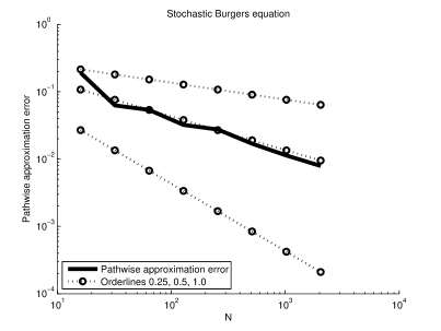
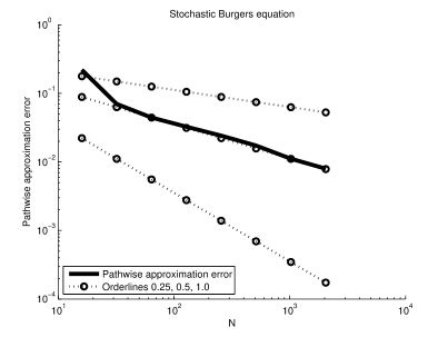
Fig. 1: Pathwise approximation error (26) against $N$ for $N\in\{16,32,64,\dots,1024,2048\}$ and two random $\omega\in\Omega$.

5 Proofs

In this section we collect all technical proofs of the previous sections.

5.1 Proof of Theorem 1

Proof.

Consider the $\mathcal{F}$/$\mathcal{B}([0,\infty))$-measurable mapping $R\colon\Omega\rightarrow[0,\infty)$ defined through

$$\begin{split}&R(\omega):=\sup_{N\in\mathbb{N}}\sup_{0\leq t\leq T}\left\|F(X^{N}_{t}(\omega))\right\|_{W}+T+\sup_{N\in\mathbb{N}}\sup_{0\leq t\leq T}\left(N^{\gamma}\left\|O_{t}(\omega)-P_{N}(O_{t}(\omega))\right\|_{V}\right)\\ &+\frac{1}{(1-\alpha)}+\sup_{N\in\mathbb{N}}\sup_{0<t\leq T}\left(t^{\alpha}\left\|P_{N}S_{t}\right\|_{L(W,V)}\right)+\sup_{N\in\mathbb{N}}\sup_{0<t\leq T}\left(t^{\alpha}N^{\gamma}\left\|S_{t}-P_{N}S_{t}\right\|_{L(W,V)}\right)\end{split}$$ (27)

for every $\omega\in\Omega$. Due to Assumptions 1-4, the mapping $R$ is indeed finite. Moreover, note that $R$ is indeed $\mathcal{F}$/$\mathcal{B}([0,\infty))$-measurable although $V$ is not assumed to be separable. Next consider the $\mathcal{B}([0,\infty))$/$\mathcal{B}([0,\infty))$-measurable mapping $L\colon[0,\infty)\rightarrow[0,\infty)$ given by $L(r):=\sup\!\left\{\frac{\|F(v)-F(w)\|_{W}}{\|v-w\|_{V}}\colon\|v\|_{V}\leq r,\ \|w\|_{V}\leq r,\ v\neq w\right\}$ for every $r\in[0,\infty)$. Additionally, consider the $\mathcal{F}$/$\mathcal{B}([0,\infty))$-measurable mapping $Z\colon\Omega\rightarrow[0,\infty)$ given by $Z(\omega):=L\!\left(\sup_{N\in\mathbb{N}}\sup_{0\leq t\leq T}\|X^{N}_{t}(\omega)\|_{V}\right)$ for every $\omega\in\Omega$. In the next step the definition of $R$ implies

$$\begin{split}\|X^{N}_{t}-X^{M}_{t}\|_{V}&\leq\Big{\|}\int^{t}_{0}P_{N}\,S_{t-s}\left(F(X^{N}_{s})-F(X^{M}_{s})\right)ds\Big{\|}_{V}\\ &+\Big{\|}\int^{t}_{0}(P_{N}-P_{M})S_{t-s}\,F(X^{M}_{s})\,ds\Big{\|}_{V}+R\left(N^{-\gamma}+M^{-\gamma}\right)\end{split}$$ (28)

for every $N,M\in\mathbb{N}$ and every $t\in[0,T]$ and the estimates $\|(P_{N}-I)\,S_{t-s}\|_{L(W,V)}\leq RN^{-\gamma}(t-s)^{-\alpha}$ and $\|P_{N}\,S_{t-s}\|_{L(W,V)}\leq R(t-s)^{-\alpha}$ for every $N,M\in\mathbb{N}$, $s\in[0,t)$ and every $t\in(0,T]$ therefore show

$$\begin{split}\|X^{N}_{t}-X^{M}_{t}\|_{V}&\leq R\int^{t}_{0}\tfrac{\|F(X^{N}_{s})-F(X^{M}_{s})\|_{W}}{(t-s)^{\alpha}}\,ds\\ &+R\left(N^{-\gamma}+M^{-\gamma}\right)\int^{t}_{0}\tfrac{\left\|F(X^{M}_{s})\right\|_{W}}{\left(t-s\right)^{\alpha}}\,ds+R\left(N^{-\gamma}+M^{-\gamma}\right)\end{split}$$ (29)

for every $N,M\in\mathbb{N}$ and every $t\in[0,T]$. Hence, we have

$$\|X^{N}_{t}-X^{M}_{t}\|_{V}\leq RZ\int^{t}_{0}\|X^{N}_{s}-X^{M}_{s}\|_{V}\,(t-s)^{-\alpha}\,ds+(R+R^{4})(N^{-\gamma}+M^{-\gamma})$$ (30)

for every $N,M\in\mathbb{N}$ and every $t\in[0,T]$ where we used the estimate $\frac{T^{(1-\alpha)}}{(1-\alpha)}\leq RT^{(1-\alpha)}\leq R^{(2-\alpha)}\leq R^{2}$ in the last inequality of (30). Lemma 7.1.11 in Henry [22] hence yields

$$\left\|X^{N}_{t}-X^{M}_{t}\right\|_{V} \leq\mathrm{E}_{(1-\alpha)}\left(t\left(R\,Z\,\Gamma(1-\alpha)\right)^{\frac{1}{(1-\alpha)}}\right)\left(R+R^{4}\right)\left(N^{-\gamma}+M^{-\gamma}\right)$$

$$\leq\mathrm{E}_{(1-\alpha)}\left(T\left(R\,Z\,\Gamma(1-\alpha)\right)^{\frac{1}{(1-\alpha)}}\right)\left(2R^{4}\right)\left(N^{-\gamma}+M^{-\gamma}\right)$$ (31)

for every $N,M\in\mathbb{N}$ and every $t\in[0,T]$. Here and below the functions $\mathrm{E}_{r}\colon[0,\infty)\rightarrow[0,\infty)$, $r\in(0,\infty)$, are defined through $\mathrm{E}_{r}(x):=\sum_{n=0}^{\infty}\frac{x^{nr}}{\Gamma(nr+1)}$ for all $x\in[0,\infty)$ and all $r\in(0,\infty)$ (see Lemma 7.1.11 in [22] for details). This shows that $\left(X^{N}(\omega)\right)_{N\in\mathbb{N}}$ is a Cauchy-sequence in $C([0,T],V)$ for every $\omega\in\Omega$. Since $C([0,T],V)$ is complete, we can define the stochastic process $X\colon[0,T]\times\Omega\rightarrow V$ with continuous sample paths by $X_{t}(\omega):=\lim_{N\rightarrow\infty}X^{N}_{t}(\omega)$ for every $t\in[0,T]$ and every $\omega\in\Omega$. Hence, we obtain

$$X_{t}(\omega)=\lim\limits_{N\rightarrow\infty}X_{t}^{N}(\omega)=\lim\limits_{N\rightarrow\infty}\left(\int^{t}_{0}P_{N}\,S_{t-s}\,F(X^{N}_{s}(\omega))\,ds+P_{N}\!\left(O_{t}(\omega)\right)\right)$$

$$=\lim\limits_{N\rightarrow\infty}\left(\int^{t}_{0}P_{N}\,S_{t-s}\,F(X^{N}_{s}(\omega))\,ds\right)+O_{t}(\omega)=\int^{t}_{0}S_{t-s}\,F(X_{s}(\omega))\,ds+O_{t}(\omega)$$

for every $t\in[0,T]$ and every $\omega\in\Omega$. Moreover, if $Y\colon[0,T]\times\Omega\rightarrow V$ is a further stochastic process with continuous sample paths and with $Y_{t}(\omega)=\int^{t}_{0}S_{t-s}\,F(Y_{s}(\omega))\,ds+O_{t}(\omega)$ for every $t\in[0,T]$ and every $\omega\in\Omega$, then we obtain

$$\begin{split}&\|X_{t}-Y_{t}\|_{V}\leq R\int^{t}_{0}(t-s)^{-\alpha}\,\|F(X_{s})-F(Y_{s})\|_{W}\,ds\\ &\leq R\cdot L\Big{(}\sup_{0\leq r\leq T}\|X_{r}\|_{V}+\sup_{0\leq r\leq T}\|Y_{r}\|_{V}\Big{)}\cdot\int^{t}_{0}(t-s)^{-\alpha}\,\|X_{s}-Y_{s}\|_{V}\,ds\end{split}$$ (32)

for every $t\in[0,T]$. Lemma 7.1.11 in [22] therefore shows that $X\colon[0,T]\times\Omega\rightarrow V$ is the pathwise unique stochastic process with continuous sample paths satisfying equation (5). Moreover, (5.1) yields $\sup_{0\leq t\leq T}\|X_{t}-X^{N}_{t}\|_{V}\leq C\cdot N^{-\gamma}$ for every $N\in\mathbb{N}$, where the $\mathcal{F}$/$\mathcal{B}[0,\infty))$-measurable mapping $C\colon\Omega\rightarrow[0,\infty)$ is given by

$$C(\omega):=2\cdot\left(R(\omega)\right)^{4}\cdot\mathrm{E}_{(1-\alpha)}\left(T\left(R(\omega)Z(\omega)\Gamma(1-\alpha)\right)^{\frac{1}{\left(1-\alpha\right)}}\right)$$ (33)

for every $\omega\in\Omega$. The proof of Theorem 1 is thus completed. ∎

5.2 Proofs for Subsection 4.1

5.2.1 Proof of Lemma 4

Throughout this subsection we use the notation $\left\|x\right\|_{2}:=\left(x_{1}^{2}+\ldots+x_{d}^{2}\right)^{\frac{1}{2}}$ for every $x=\left(x_{1},\ldots,x_{d}\right)\in\mathbb{R}^{d}$. We first present three elementary lemmas, which we need in the proof of Lemma 4. They are, for example, proved as Lemmas 9, 11 and 12 in [24].

Lemma 10.

It holds that $\int_{(0,1)^{d}}\int_{(0,1)^{d}}\frac{1}{\left\|x-y\right\|_{2}^{\alpha}}\,dx\,dy\leq\frac{\left(3d\right)^{d}}{\left(d-\alpha\right)}$ for every $\alpha\in(0,d)$ and every $d\in\mathbb{N}$.

Lemma 11.

Let $d\in\mathbb{N}$ and let $e_{i}\in C([0,1]^{d},\mathbb{R})$, $i\in\mathbb{N}^{d}$, be given by (7). Then $\left|e_{i}(x)-e_{i}(y)\right|\leq 2^{\frac{d}{2}}\pi\|i\|_{2}\|x-y\|_{2}$ for every $x,y\in[0,1]^{d}$ and every $i\in\mathbb{N}^{d}$.

Lemma 12.

Let $\beta\colon[0,T]\times\Omega\rightarrow\mathbb{R}$ be a standard Brownian motion. Then $\mathbb{E}\!\left[|\int^{t_{2}}_{0}e^{-\lambda(t_{2}-s)}\,d\beta_{s}-\int^{t_{1}}_{0}e^{-\lambda(t_{1}-s)}\,d\beta_{s}|^{2}\right]\leq\lambda^{\left(r-1\right)}\left|t_{2}-t_{1}\right|^{r}$ for every $t_{1},t_{2}\in[0,T]$, $r\in[0,1]$ and every $\lambda\in(0,\infty)$.

After these three very simple lemmas, we present now two lemmas (Lemma 13 and Lemma 14), which are the essential constituents in the proof of Lemma 4. The first one will ensure the temporal regularity of the processes that are constructed in Lemma 4.

Lemma 13.

Let $d\in\mathbb{N}$, let $\beta^{i}\colon[0,T]\times\Omega\rightarrow\mathbb{R}$, $i\in\mathbb{N}^{d}$, be a family of independent standard Brownian motions and let $b\colon\mathbb{N}^{d}\rightarrow\mathbb{R}$ be an arbitrary function. Then

$$\Big{(}\mathbb{E}\Big{[}\sup_{x\in[0,1]^{d}}\left|O^{N}_{t_{2}}(x)-O^{N}_{t_{1}}(x)\right|^{p}\Big{]}\Big{)}^{\!\frac{1}{p}}\leq C_{\star}\left[\sum_{i\in\{1,\dots,N\}^{d}}|b(i)|^{2}\,\|i\|_{2}^{(4\theta+4\alpha-2)}\right]^{\!\frac{1}{2}}\left|t_{2}-t_{1}\right|^{\theta}$$ (34)

for every $t_{1},t_{2}\in[0,T]$, $N\in\mathbb{N}$, $p\in[1,\infty)$ and every $\alpha$, $\theta\in(0,\frac{1}{2}]$, where $C_{\star}\in[0,\infty)$ is a constant which depends on $d,p,\alpha$ and $\theta$ only and where the stochastic process $O^{N}\colon[0,T]\times\Omega\rightarrow C([0,1]^{d},\mathbb{R})$ is defined through

$$O^{N}_{t}(\omega):=\sum_{i\in\{1,\dots,N\}^{d}}b(i)\Big{(}-\lambda_{i}\int^{t}_{0}e^{-\lambda_{i}(t-s)}\beta^{i}_{s}(\omega)\,ds+\beta^{i}_{t}(\omega)\Big{)}\cdot e_{i}$$ (35)

for every $t\in[0,T]$, $\omega\in\Omega$ and every $N\in\mathbb{N}$. Here $e_{i}\in C([0,1]^{d},\mathbb{R})$, $i\in\mathbb{N}^{d}$, and $\lambda_{i}\in\mathbb{R}$, $i\in\mathbb{N}^{d}$, are given in (7).

Proof.

Throughout this proof let $\alpha,\theta\in(0,\frac{1}{2}]$, $p,N\in\mathbb{N}$ with $p>\frac{1}{\alpha}$ and $t_{1},t_{2}\in[0,T]$ with $t_{1}\leq t_{2}$ be fixed. In addition, let $C=C_{d,p,\alpha,\theta}\in[0,\infty)$ be a constant which changes from line to line but depends on $d$, $p$, $\alpha$ and $\theta$ only. We show now inequality (34) for these parameters and the case with a general $p\in[1,\infty)$ then follows from Jensen’s inequality. The definition of $O^{N}$ implies

$$\begin{split}&(O^{N}_{t_{2}}(x)-O^{N}_{t_{1}}(x))-(O^{N}_{t_{2}}(y)-O^{N}_{t_{1}}(y))\\ &=\sum_{i\in\{1,\dots,N\}^{d}}\!\!\!b(i)\Big{(}\int^{t_{2}}_{0}e^{-\lambda_{i}(t_{2}-s)}\,d\beta^{i}_{s}-\int^{t_{1}}_{0}e^{-\lambda_{i}(t_{1}-s)}\,d\beta^{i}_{s}\Big{)}\cdot(e_{i}(x)-e_{i}(y))\end{split}$$ (36)

$\mathbb{P}$-a.s. for every $x,y\in[0,1]^{d}$. Hence, Lemma 11 and Lemma 12 yield

$$\mathbb{E}\Big{[}\left|(O^{N}_{t_{2}}(x)-O^{N}_{t_{1}}(x))-(O^{N}_{t_{2}}(y)-O^{N}_{t_{1}}(y))\right|^{2}\Big{]}$$

$$=\sum_{i\in\{1,\dots,N\}^{d}}|b(i)|^{2}\,\mathbb{E}\!\left[\Big{|}\int^{t_{2}}_{0}e^{-\lambda_{i}(t_{2}-s)}\,d\beta^{i}_{s}-\int^{t_{1}}_{0}e^{-\lambda_{i}(t_{1}-s)}\,d\beta^{i}_{s}\Big{|}^{2}\right]|e_{i}(x)-e_{i}(y)|^{2}$$

$$\leq\sum_{i\in\{1,\dots,N\}^{d}}|b(i)|^{2}\,|\lambda_{i}|^{(2\theta-1)}\,|t_{2}-t_{1}|^{2\theta}\left(2^{d}\pi^{2}\|i\|_{2}^{2}\|x-y\|_{2}^{2}\right)^{2\alpha}\left(\left|e_{i}(x)\right|+\left|e_{i}(y)\right|\right)^{2\left(1-2\alpha\right)}$$

$$\leq C\,|t_{2}-t_{1}|^{2\theta}\,\|x-y\|_{2}^{4\alpha}\sum\nolimits_{i\in\{1,\dots,N\}^{d}}|b(i)|^{2}\,\|i\|_{2}^{(4\theta+4\alpha-2)}$$ (37)

for every $x,y\in[0,1]^{d}$. Moreover, Lemma 12 gives

$$\begin{split}&\mathbb{E}\!\left[|O^{N}_{t_{2}}(x)-O^{N}_{t_{1}}(x)|^{2}\right]\\ &=\sum_{i\in\{1,\dots,N\}^{d}}|b(i)|^{2}\,\mathbb{E}\!\left[\Big{|}\int^{t_{2}}_{0}e^{-\lambda_{i}(t_{2}-s)}\,d\beta^{i}_{s}-\int^{t_{1}}_{0}e^{-\lambda_{i}(t_{1}-s)}\,d\beta^{i}_{s}\Big{|}^{2}\right]|e_{i}(x)|^{2}\\ &\leq C\!\!\sum_{i\in\{1,\dots,N\}^{d}}|b(i)|^{2}\,\|i\|_{2}^{(4\theta-2)}\,|t_{2}-t_{1}|^{2\theta}\end{split}$$ (38)

for every $x\in[0,1]^{d}$. In the next step the Sobolev embeddings in Subsections 2.2.4 and 2.4.4 in [38] yield

$$\mathbb{E}\big{[}\|O^{N}_{t_{2}}-O^{N}_{t_{1}}\|_{C([0,1]^{d},\mathbb{R})}^{p}\big{]}$$

$$\leq C\int_{(0,1)^{d}}\int_{(0,1)^{d}}\frac{\mathbb{E}\big{[}|(O^{N}_{t_{2}}(x)-O^{N}_{t_{1}}(x))-(O^{N}_{t_{2}}(y)-O^{N}_{t_{1}}(y))|^{p}\big{]}}{\|x-y\|_{2}^{d+p\alpha}}\,dx\,dy$$

$$\quad+C\int_{(0,1)^{d}}\mathbb{E}\big{[}|O^{N}_{t_{2}}(x)-O^{N}_{t_{1}}(x)|^{p}\big{]}\,dx$$

$$\leq C\int_{(0,1)^{d}}\int_{(0,1)^{d}}\frac{\left(\mathbb{E}\big{[}|(O^{N}_{t_{2}}(x)-O^{N}_{t_{1}}(x))-(O^{N}_{t_{2}}(y)-O^{N}_{t_{1}}(y))|^{2}\big{]}\right)^{\!\frac{p}{2}}}{\|x-y\|_{2}^{d+p\alpha}}dx\,dy$$

$$\quad+C\int_{(0,1)^{d}}\left(\mathbb{E}\big{[}|O^{N}_{t_{2}}(x)-O^{N}_{t_{1}}(x)|^{2}\big{]}\right)^{\!\frac{p}{2}}dx$$

and (37) and (38) therefore show

$$\mathbb{E}\|O^{N}_{t_{2}}-O^{N}_{t_{1}}\|_{C([0,1]^{d},\mathbb{R})}^{p}$$

$$\leq C\int_{(0,1)^{d}}\int_{(0,1)^{d}}\frac{|t_{2}-t_{1}|^{p\theta}\,\|x-y\|_{2}^{2p\alpha}}{\|x-y\|_{2}^{d+p\alpha}}\,dx\,dy\Big{(}\sum\nolimits_{i\in\{1,\dots,N\}^{d}}|b(i)|^{2}\,\|i\|_{2}^{(4\theta+4\alpha-2)}\Big{)}^{\!\frac{p}{2}}$$

$$\quad+C\Big{(}\sum\nolimits_{i\in\{1,\dots,N\}^{d}}|b(i)|^{2}\,\|i\|_{2}^{(4\theta-2)}\,|t_{2}-t_{1}|^{2\theta}\Big{)}^{\!\frac{p}{2}}$$

$$\leq C\Big{(}1+\int_{(0,1)^{d}}\int_{(0,1)^{d}}\|x-y\|_{2}^{p\alpha-d}\,dx\,dy\Big{)}|t_{2}-t_{1}|^{p\theta}\Big{(}\sum_{i\in\{1,\dots,N\}^{d}}|b(i)|^{2}\|i\|_{2}^{4\theta+4\alpha-2}\Big{)}^{\!\frac{p}{2}}.$$

Lemma 10 hence gives

$$\left(\mathbb{E}\!\left[\left\|O^{N}_{t_{2}}-O^{N}_{t_{1}}\right\|_{C([0,1]^{d},\mathbb{R})}^{p}\right]\right)^{\!\frac{1}{p}}\leq C\Big{(}\sum_{i\in\left\{1,\dots,N\right\}^{d}}|b(i)|^{2}\,\|i\|_{2}^{(4\theta+4\alpha-2)}\Big{)}^{\!\frac{1}{2}}\left|t_{2}-t_{1}\right|^{\theta}$$ (39)

and this completes the proof of Lemma 13. ∎

Lemma 14.

Let $d\in\mathbb{N}$, let $\beta^{i}\colon[0,T]\times\Omega\rightarrow\mathbb{R}$, $i\in\mathbb{N}^{d}$, be a family of independent standard Brownian motions and let $b\colon\mathbb{N}^{d}\rightarrow\mathbb{R}$ be an arbitrary function. Then

$$\Big{(}\mathbb{E}\Big{[}\sup_{0\leq t\leq T}\sup_{x\in[0,1]^{d}}\left|O^{N}_{t}(x)-O^{M}_{t}(x)\right|^{p}\Big{]}\Big{)}^{\!\frac{2}{p}}\leq C_{\star}\!\!\!\!\!\!\!\!\sum_{i\in\left\{1,\dots,N\right\}^{d}\backslash\{1,\dots,M\}^{d}}\!\!\!\!\!\!\!\!|b(i)|^{2}\,\|i\|_{2}^{\left(8\alpha-2\right)}$$ (40)

for every $N,M\in\mathbb{N}$ with $N\geq M$, every $p\in[1,\infty)$ and every $\alpha\in\left(0,\frac{1}{2}\right)$, where $C_{\star}\in[0,\infty)$ is a constant which depends on $d$, $p$, $\alpha$ and $T$ only and where $O^{N}\colon[0,T]\times\Omega\rightarrow C([0,1]^{d},\mathbb{R})$, $N\in\mathbb{N}$, are stochastic processes defined through (35).

Proof.

Throughout this proof let $\alpha\in(0,\frac{1}{2})$ and $p,N,M\in\mathbb{N}$ with $p>\frac{1}{\alpha}$ and $N\geq M$ be fixed. In addition, let $C=C_{d,p,\alpha,T}\in[0,\infty)$ be a constant, which changes from line to line but which depends on $d$, $p$, $\alpha$ and $T$ only. As in the proof of Lemma 13, we show now inequality (40) for these parameters and the case with a general $p\in[1,\infty)$ then follows from Jensen’s inequality. We use the factorization method (see [12] and, e.g., Section 5.3 in [13] and Section 5 in [5]) to show (40). For this let $Y^{N,M}\colon[0,T]\times\Omega\rightarrow C([0,1]^{d},\mathbb{R})$ be a stochastic processes with continuous sample paths given by

$$Y^{N,M}_{t}=\sum_{i\in\{1,\dots,N\}^{d}\backslash\{1,\dots,M\}^{d}}b(i)\int^{t}_{0}\left(t-s\right)^{-\alpha}e^{-\lambda_{i}(t-s)}\,d\beta^{i}_{s}\cdot e_{i}$$ (41)

$\mathbb{P}$-a.s. for every $t\in[0,T]$. By using Kolmogorov’s theorem (see, e.g., Theorem 3.3 in [13]), one can check in a straightforward way that the stochastic processes $\int^{t}_{0}(t-s)^{-\alpha}\,e^{\lambda_{i}(t-s)}\,d\beta^{i}_{s}$, $t\in[0,T]$, $i\in\mathbb{N}^{d}$, indeed have modifications with continuous sample paths. The key idea of the factorization method is then to make use of the identity

$$O^{N}_{t}-O^{M}_{t}=\frac{\sin(\pi\alpha)}{\pi}\int^{t}_{0}(t-s)^{(\alpha-1)}\,S_{t-s}\,Y^{N,M}_{s}\,ds$$ (42)

$\mathbb{P}$-a.s. for every $t\in[0,T]$ (see, e.g., equation (5.18) in Section 5.3 in [13]). More precisely, combining (42), the well known fact $\sup_{0\leq t\leq T}\|S_{t}\|_{L(C([0,1]^{d},\mathbb{R}))}\leq 1$ (see, e.g., Lemma 6 in [24]) and Hölder’s inequality gives

$$\begin{split}&\mathbb{E}\sup_{0\leq t\leq T}\left\|O^{N}_{t}-O^{M}_{t}\right\|_{C([0,1]^{d},\mathbb{R})}^{p}\\ &=\mathbb{E}\sup_{0\leq t\leq T}\Big{\|}\frac{\sin(\pi\alpha)}{\pi}\int^{t}_{0}(t-s)^{(\alpha-1)}\,S_{t-s}\,Y^{N,M}_{s}\,ds\Big{\|}_{C([0,1]^{d},\mathbb{R})}^{p}\\ &\leq\mathbb{E}\sup_{0\leq t\leq T}\Big{|}\int^{t}_{0}(t-s)^{(\alpha-1)}\,\|Y^{N,M}_{s}\|_{C([0,1]^{d},\mathbb{R})}\,ds\Big{|}^{p}\\ &\leq C\int^{T}_{0}\mathbb{E}\!\left[\|Y^{N,M}_{s}\|_{C([0,1]^{d},\mathbb{R})}^{p}\right]ds\;.\end{split}$$ (43)

Hence, it remains to bound $\|Y^{N,M}_{s}\|_{C([0,1]^{d},\mathbb{R})}$ in (43). For this, denote $\mathcal{I}_{N}:=\{1,2,\dots,N\}^{d}$ and $\mathcal{I}_{M}:=\{1,2,\dots,M\}^{d}$. Lemma 11 then implies

$$\begin{split}&\mathbb{E}\big{[}|Y^{N,M}_{t}(x)-Y^{N,M}_{t}(y)|^{2}\big{]}\\ &=\mathbb{E}\Big{[}\Big{|}\sum_{i\in\mathcal{I}_{N}\backslash\mathcal{I}_{M}}b(i)\int^{t}_{0}(t-s)^{-\alpha}\,e^{-\lambda_{i}(t-s)}\,d\beta^{i}_{s}\cdot(e_{i}(x)-e_{i}(y))\Big{|}^{2}\Big{]}\\ &=\sum_{i\in\mathcal{I}_{N}\backslash\mathcal{I}_{M}}|b(i)|^{2}\;\mathbb{E}\Big{[}\Big{|}\int^{t}_{0}(t-s)^{-\alpha}\,e^{-\lambda_{i}(t-s)}\,d\beta^{i}_{s}\Big{|}^{2}\Big{]}\cdot|e_{i}(x)-e_{i}(y)|^{2}\\ &=\sum_{i\in\mathcal{I}_{N}\backslash\mathcal{I}_{M}}|b(i)|^{2}\int^{t}_{0}s^{-2\alpha}\,e^{-2\lambda_{i}s}\,ds\cdot|e_{i}(x)-e_{i}(y)|^{4\alpha}\,|e_{i}(x)-e_{i}(y)|^{(2-4\alpha)}\\ &\leq C\sum_{i\in\mathcal{I}_{N}\backslash\mathcal{I}_{M}}|b(i)|^{2}\,\|i\|_{2}^{(8\alpha-2)}\left\|x-y\right\|_{2}^{4\alpha}\end{split}$$ (44)

for every $t\in[0,T]$ and every $x,y\in[0,1]^{d}$. In addition, note that

$$\begin{split}&\mathbb{E}\!\left[|Y^{N,M}_{t}(x)|^{2}\right]=\mathbb{E}\Big{[}\Big{|}\sum_{i\in\mathcal{I}_{N}\backslash\mathcal{I}_{M}}b(i)\int^{t}_{0}(t-s)^{-\alpha}\,e^{-\lambda_{i}(t-s)}\,d\beta^{i}_{s}\cdot e_{i}(x)\Big{|}^{2}\Big{]}\\ &=\sum_{i\in\mathcal{I}_{N}\backslash\mathcal{I}_{M}}|b(i)|^{2}\;\mathbb{E}\Big{[}\Big{|}\int^{t}_{0}(t-s)^{-\alpha}\,e^{-\lambda_{i}(t-s)}\,d\beta^{i}_{s}\Big{|}^{2}\Big{]}|e_{i}(x)|^{2}\\ &=\sum_{i\in\mathcal{I}_{N}\backslash\mathcal{I}_{M}}|b(i)|^{2}\int^{2t\lambda_{i}}_{0}s^{-2\alpha}\,e^{-s}\,ds(2\lambda_{i})^{(2\alpha-1)}\,|e_{i}(x)|^{2}\leq C\!\!\!\sum_{i\in\mathcal{I}_{N}\backslash\mathcal{I}_{M}}|b(i)|^{2}\,\|i\|_{2}^{(8\alpha-2)}\end{split}$$ (45)

for every $t\in[0,T]$ and every $x,y\in[0,1]^{d}$. In the next step the Sobolev embeddings in Subsections 2.2.4 and 2.4.4 in [38] give

$$\begin{split}\sup_{0\leq t\leq T}\mathbb{E}\|Y^{N,M}_{t}\|_{C([0,1]^{d},\mathbb{R})}^{p}&\leq C\sup_{0\leq t\leq T}\int_{(0,1)^{d}}\int_{(0,1)^{d}}\frac{\big{(}\mathbb{E}\big{[}|Y^{N,M}_{t}(x)-Y^{N,M}_{t}(y)|^{2}\big{]}\big{)}^{{p/2}}}{\|x-y\|_{2}^{d+p\alpha}}\,dx\,dy\\ &\quad+C\sup_{0\leq t\leq T}\int_{(0,1)^{d}}\left(\mathbb{E}\big{[}|Y^{N,M}_{t}(x)|^{2}\big{]}\right)^{\!\frac{p}{2}}dx\end{split}$$ (46)

and (44), (45) and Lemma 10 therefore imply

$$\begin{split}&\sup_{0\leq t\leq T}\mathbb{E}\big{[}\|Y^{N,M}_{t}\|_{C([0,1]^{d},\mathbb{R})}^{p}\big{]}\\ &\leq C\int_{(0,1)^{d}}\int_{(0,1)^{d}}\frac{\left(\sum_{i\in\mathcal{I}_{N}\backslash\mathcal{I}_{M}}|b(i)|^{2}\,\|i\|_{2}^{(8\alpha-2)}\,\|x-y\|_{2}^{4\alpha}\right)^{\frac{p}{2}}}{\|x-y\|^{(d+p\alpha)}}\,dx\,dy\\ &\quad+C\Big{(}\sum_{i\in\mathcal{I}_{N}\backslash\mathcal{I}_{M}}|b(i)|^{2}\,\|i\|_{2}^{(8\alpha-2)}\Big{)}^{p/2}\leq C\Big{(}\sum_{i\in\mathcal{I}_{N}\backslash\mathcal{I}_{M}}|b(i)|^{2}\,\|i\|_{2}^{(8\alpha-2)}\Big{)}^{p/2}.\end{split}$$ (47)

This and inequality (43) then show (40). The proof of Lemma 14 is thus completed. ∎

Proof of Lemma 4.

Throughout this proof let $O^{N}\colon[0,T]\times\Omega\rightarrow C([0,1]^{d},\mathbb{R})$, $N\in\mathbb{N}$, be a sequence of stochastic processes defined through (35). Next note that Lemma 14 implies

$$\begin{split}\left(\mathbb{E}\!\left[\sup_{0\leq t\leq T}\|O^{N}_{t}-O^{M}_{t}\|_{C([0,1]^{d},\mathbb{R})}^{p}\right]\right)^{\!\frac{1}{p}}&\leq C\Big{(}\sum_{i\in\mathbb{N}^{d}\backslash\{1,\dots,M\}^{d}}|b(i)|^{2}\,\|i\|_{2}^{(8\alpha-2)}\Big{)}^{\!\frac{1}{2}}\\ &\leq C\Big{(}\sum_{i\in\mathbb{N}^{d}}|b(i)|^{2}\,\|i\|_{2}^{(2\rho-2)}\Big{)}^{\!\frac{1}{2}}M^{(4\alpha-\rho)}\end{split}$$ (48)

for every $N,M\in\mathbb{N}$ with $N\geq M$, every $p\in[1,\infty)$ and every $\alpha\in(0,\min(\frac{1}{2},\frac{\rho}{4}))$ where $C\in[0,\infty)$ is a constant which depends on $d$, $p$, $\alpha$ and $T$ only. This, in particular, gives that $O^{N}\colon[0,T]\times\Omega\rightarrow C([0,1]^{d},\mathbb{R})$, $N\in\mathbb{N}$, is a Cauchy sequence in $L^{p}(\Omega;C([0,T],C([0,1]^{d},\mathbb{R})))$. Hence, there exists a stochastic process $\tilde{O}\colon[0,T]\times\Omega\rightarrow C([0,1]^{d},\mathbb{R})$ with continuous sample paths which satisfies

$$\Big{(}\mathbb{E}\Big{[}\sup_{0\leq t\leq T}\|\tilde{O}_{t}-O^{N}_{t}\|_{C([0,1]^{d},\mathbb{R})}^{p}\Big{]}\Big{)}^{\!\frac{1}{p}}\leq C\Big{(}\sum_{i\in\mathbb{N}^{d}}|b(i)|^{2}\,\|i\|_{2}^{(2\rho-2)}\Big{)}^{\!\frac{1}{2}}N^{(4\alpha-\rho)}$$ (49)

for every $N\in\mathbb{N}$, every $p\in[1,\infty)$ and every $\alpha\in(0,\min(\frac{1}{2},\frac{\rho}{4}))$. Therefore, we have

$$\sup_{N\in\mathbb{N}}\left\{N^{\gamma}\left(\mathbb{E}\!\left[\sup_{0\leq t\leq T}\|\tilde{O}_{t}-O^{N}_{t}\|_{C([0,1]^{d},\mathbb{R})}^{p}\right]\right)^{\!\frac{1}{p}}\right\}<\infty$$ (50)

for every $\gamma\in(0,\rho)$ and every $p\in[1,\infty)$. This implies

$$\mathbb{P}\!\left[\,\sup_{N\in\mathbb{N}}\left(N^{\gamma}\sup_{0\leq t\leq T}\|\tilde{O}_{t}-O^{N}_{t}\|_{C([0,1]^{d},\mathbb{R})}\right)<\infty\,\right]=1$$ (51)

for every $\gamma\in(0,\rho)$ due to Lemma 2.1 in [27]. This yields

$$\mathbb{P}\!\left[\;\forall\;\gamma\in(0,\rho)\colon\sup_{N\in\mathbb{N}}\,\sup_{0\leq t\leq T}\left(N^{\gamma}\,\|\tilde{O}_{t}-O^{N}_{t}\|_{C([0,1]^{d},\mathbb{R})}\right)<\infty\;\right]=1$$ (52)

and hence, we obtain that

$$\mathbb{P}\!\left[\;\lim_{N\rightarrow\infty}\,\sup_{0\leq t\leq T}\|\tilde{O}_{t}-O^{N}_{t}\|_{C([0,1]^{d},\mathbb{R})}=0\;\right]=1\qquad\text{and}$$ (53)

$$\mathbb{P}\!\left[\;\forall\;\gamma\in(0,\rho)\colon\sup_{N\in\mathbb{N}}\,\sup_{0\leq t\leq T}\left(N^{\gamma}\,\|\tilde{O}_{t}-P_{N}(\tilde{O}_{t})\|_{C([0,1]^{d},\mathbb{R})}\right)<\infty\;\right]=1.$$ (54)

In addition, Lemma 13 gives

$$\Big{(}\mathbb{E}\Big{[}\|O^{N}_{t_{2}}-O^{N}_{t_{1}}\|_{C([0,1]^{d},\mathbb{R})}^{p}\Big{]}\Big{)}^{\!\frac{1}{p}} \leq\tilde{C}_{d,p,\rho,\theta}\Big{(}\sum_{i\in\{1,\dots,N\}^{d}}|b(i)|^{2}\,\|i\|_{2}^{4\theta+4(\frac{\rho}{2}-\theta)-2}\Big{)}^{\!\frac{1}{2}}\left|t_{2}-t_{1}\right|^{\theta}$$

$$\leq\tilde{C}_{d,p,\rho,\theta}\Big{(}\sum_{i\in\mathbb{N}^{d}}|b(i)|^{2}\,\|i\|_{2}^{(2\rho-2)}\Big{)}^{\!\frac{1}{2}}\left|t_{2}-t_{1}\right|^{\theta}$$

for every $t_{1},t_{2}\in[0,T]$, $N\in\mathbb{N}$, $p\in[1,\infty)$ and every $\theta\in(0,\frac{\rho}{2})\cap[0,\frac{1}{2}]$ where $\tilde{C}_{d,p,\rho,\theta}\in[0,\infty)$ is a constant which depends on $d$, $p$, $\rho$ and $\theta$ only. This shows

$$\left(\mathbb{E}\!\left[\|\tilde{O}_{t_{2}}-\tilde{O}_{t_{1}}\|_{C([0,1]^{d},\mathbb{R})}^{p}\right]\right)^{\!\frac{1}{p}}\leq\tilde{C}_{d,p,\rho,\theta}\Big{(}\sum_{i\in\mathbb{N}^{d}}|b(i)|^{2}\,\|i\|_{2}^{2\rho-2}\Big{)}^{\!\frac{1}{2}}|t_{2}-t_{1}|^{\theta}$$ (55)

for every $t_{1},t_{2}\in[0,T]$, $p\in[1,\infty)$ and every $\theta\in\left(0,\frac{\rho}{2}\right)$, $\theta\leq\frac{1}{2}$. Kolmogorov’s theorem (see, e.g., Theorem 3.3 in [13]) hence yields

$$\mathbb{P}\!\left[\sup_{0\leq t_{1}<t_{2}\leq T}\frac{\|\tilde{O}_{t_{2}}-\tilde{O}_{t_{1}}\|_{C([0,1]^{d},\mathbb{R})}}{|t_{2}-t_{1}|^{\theta}}<\infty\right]=1$$ (56)

for every $\theta\in\left(0,\min\left(\frac{1}{2},\frac{\rho}{2}\right)\right)$. This implies

$$\mathbb{P}\!\left[\,\forall\;\theta\in(0,\min\{\tfrac{1}{2},\tfrac{\rho}{2}\})\colon\sup_{0\leq t_{1}<t_{2}\leq T}\frac{\|\tilde{O}_{t_{2}}-\tilde{O}_{t_{1}}\|_{C([0,1]^{d},\mathbb{R})}}{\left|t_{2}-t_{1}\right|^{\theta}}<\infty\,\right]=1.$$ (57)

Combining (54) and (57) shows the existence of a stochastic process $O\colon[0,T]\times\Omega\rightarrow C([0,1]^{d},\mathbb{R})$ with continuous sample paths which is indistinguishable from $\tilde{O}$, i.e., $\mathbb{P}\big{[}\,\forall\,t\in[0,T]\colon O_{t}=\tilde{O}_{t}\,\big{]}=1$ and which satisfies $\sup_{0\leq t_{1}<t_{2}\leq T}\frac{\|O_{t_{2}}(\omega)-O_{t_{1}}(\omega)\|_{C([0,1]^{d},\mathbb{R})}}{\left|t_{2}-t_{1}\right|^{\theta}}$ $<\infty$ and $\sup_{N\in\mathbb{N}}\sup_{0\leq t\leq T}\left(N^{\gamma}\left\|O_{t}(\omega)-P_{N}(O_{t}(\omega))\right\|_{C([0,1]^{d},\mathbb{R})}\right)<\infty$ for every $\omega\in\Omega$, every $\theta\in\left(0,\min\left(\frac{1}{2},\frac{\rho}{2}\right)\right)$ and every $\gamma\in(0,\rho)$. The proof of Lemma 4 is thus completed. ∎

5.3 Proofs for Subsection 4.3

5.3.1 Proof of Lemma 7

Proof.

First, note that

$$\sum^{\infty}_{n=1}n^{2+2\gamma}\,e^{-2n^{2}\pi^{2}t}\leq\int^{\infty}_{0}(x+1)^{2+2\gamma}e^{-2x^{2}\pi^{2}t}\,dx$$

$$\leq\int^{\infty}_{0}8\big{(}x^{2+2\gamma}+1)e^{-2x^{2}\pi^{2}t}\,dx=\frac{1}{2\pi\sqrt{t}}\int^{\infty}_{0}8\Big{(}\frac{x^{2+2\gamma}}{(2\pi\sqrt{t})^{2+2\gamma}}+1\Big{)}e^{-\frac{x^{2}}{2}}dx$$

$$\leq\frac{4}{\pi\sqrt{t}}\int^{\infty}_{0}\Big{(}\frac{x^{2+2\gamma}}{t^{1+\gamma}}+1\Big{)}e^{-\frac{x^{2}}{2}}dx\leq\frac{4}{\pi\sqrt{t}}\int^{\infty}_{0}\left(\frac{x^{4}+1}{t^{1+\gamma}}+\frac{T^{1+\gamma}}{t^{1+\gamma}}\right)e^{-\frac{x^{2}}{2}}dx$$

$$\leq\frac{4\sqrt{2\pi}}{t^{\frac{3}{2}+\gamma}\pi}\int_{\mathbb{R}}\frac{x^{4}+T^{2}+2}{\sqrt{2\pi}}\,e^{-\frac{x^{2}}{2}}dx\leq\frac{4(T^{2}+5)}{t^{\frac{3}{2}+\gamma}}$$

for every $t\in(0,T]$ and every $\gamma\in[0,\frac{1}{2})$. The identity $\|w\|_{H^{-1}}$ $=$ $\sum^{\infty}_{n=1}n^{-2}\pi^{-2}$ $|w(\sqrt{2}\sin(n\pi\cdot))|^{2}$ for every $w\in H^{-1}((0,1),\mathbb{R})$ hence gives

$$\sup_{0\leq x\leq 1}\Big{(}\sum^{\infty}_{n=N}2\cdot e^{-n^{2}\pi^{2}t}\cdot|w(\sin(n\pi(\cdot)))|\cdot|\sin(n\pi x)|\Big{)}$$

$$\leq\pi\sqrt{2}\sum^{\infty}_{n=N}n\,e^{-n^{2}\pi^{2}t}\,\frac{|w(\sqrt{2}\sin(n\pi(\cdot)))|}{n\pi}$$

$$\leq\pi\sqrt{2}\Big{(}\sum^{\infty}_{n=N}n^{2}\,e^{-2n^{2}\pi^{2}t}\Big{)}^{\!\frac{1}{2}}\|w\|_{H^{-1}}\leq\pi\sqrt{2}\,N^{-\gamma}\Big{(}\sum^{\infty}_{n=N}n^{(2+2\gamma)}\,e^{-2n^{2}\pi^{2}t}\Big{)}^{\!\frac{1}{2}}\|w\|_{H^{-1}}$$

$$\leq\pi\sqrt{2}\,N^{-\gamma}\left(4\left(T^{2}+5\right)t^{-\left(\frac{3}{2}+\gamma\right)}\right)^{\frac{1}{2}}\|w\|_{H^{-1}}\leq 10\left(T+3\right)t^{-(\frac{3}{4}+\frac{\gamma}{2})}N^{-\gamma}\,\|w\|_{H^{-1}}$$

for every $w\in H^{-1}((0,1),\mathbb{R})$, $N\in\mathbb{N}$, $\gamma\in[0,\frac{1}{2})$ and every $t\in(0,T]$. This implies $\|S_{t}(w)\|_{C([0,1],\mathbb{R})}\leq 10\,(T+3)\,t^{-\frac{3}{4}}\,\|w\|_{H^{-1}}$ and

$$\|S_{t}(w)-P_{N}(S_{t}(w))\|_{C([0,1],\mathbb{R})}\leq\frac{10\left(T+3\right)\|w\|_{H^{-1}}}{t^{\left(\frac{3}{4}+\frac{\gamma}{2}\right)}\left(N+1\right)^{\gamma}}\leq\frac{10\left(T+3\right)\|w\|_{H^{-1}}}{t^{\left(\frac{3}{4}+\frac{\gamma}{2}\right)}N^{\gamma}}$$ (58)

for every $t\in(0,T]$, $w\in H^{-1}\left((0,1),\mathbb{R}\right)$, $\gamma\in[0,\frac{1}{2})$ and every $N\in\mathbb{N}$. Therefore, we finally obtain $\sup_{0<t\leq T}\big{(}t^{\frac{3}{4}}\left\|S_{t}\right\|_{L(H^{-1}((0,1),\mathbb{R}),\,C([0,1],\mathbb{R}))}\big{)}<\infty$ and

$$\sup_{N\in\mathbb{N}}\sup_{0<t\leq T}\Big{(}t^{\left(\frac{3}{4}+\frac{\gamma}{2}\right)}N^{\gamma}\left\|S_{t}-P_{N}S_{t}\right\|_{L(H^{-1}((0,1),\mathbb{R}),\,C([0,1],\mathbb{R}))}\Big{)}<\infty$$ (59)

for every $\gamma\in[0,\frac{1}{2})$. The proof of Lemma 7 is thus completed. ∎

5.3.2 Proof of Lemma 9

In the proof of Lemma 9 the following well known estimates for the analytic semigroup generated by the Laplacian are used. Their proofs can, e.g., be found in Lemma 5.8 in [3].

Lemma 15.

Let $S\colon(0,T]\rightarrow L\big{(}H^{-1}((0,1),\mathbb{R}),C([0,1],\mathbb{R})\big{)}$ be given by Lemma 7 and let $P_{N}\colon C([0,1],\mathbb{R})\rightarrow C([0,1],\mathbb{R})$, $N\in\mathbb{N}$, be given by (20). Then

$$\|P_{N}S_{t}\|_{L(L^{2}((0,1),\mathbb{R}),C([0,1],\mathbb{R}))}\leq t^{-\frac{1}{4}}\,,\qquad\left\|P_{N}S_{t}\right\|_{L(L^{2}((0,1),\mathbb{R}),L^{4}((0,1),\mathbb{R}))}\leq t^{-\frac{1}{8}}\;,$$

$$\|S_{t}\|_{L(H^{-1}((0,1),\mathbb{R}),L^{2}((0,1),\mathbb{R}))}\leq t^{-\frac{1}{2}}\,\quad\text{and}\quad\|S_{t}(v^{\prime})\|_{L^{2}}\leq 4\,(t+1)\,t^{-\frac{3}{4}}\,\|v\|_{L^{1}}$$

for every $t\in(0,T],N\in\mathbb{N}$ and every $v\in C^{1}([0,1],\mathbb{R})$.

In addition to Lemma 15, the following elementary global coercivity estimate for Burgers equation is used in the proof of Lemma 9 (see also Lemma 3.1 in [10]).

Lemma 16.

Let $F\colon C([0,1],\mathbb{R})\rightarrow H^{-1}((0,1),\mathbb{R})$ be given by Lemma 8. Then

$$\left<v,v^{\prime\prime}+F(v+w)\right>_{L^{2}}\leq 2\,c^{2}\|v\|^{2}_{L^{2}}\|w\|^{2}_{C([0,1],\mathbb{R})}+2\,c^{2}\|w\|^{4}_{C([0,1],\mathbb{R})}$$ (60)

for all twice continuously differentiable functions $v\colon[0,1]\rightarrow\mathbb{R}$ and $w\colon[0,1]\rightarrow\mathbb{R}$ with $v(0)=v(1)=0$ and where $c\in\mathbb{R}$ is used in Lemma 8.

Proof.

Integration by parts and the identity $\int_{0}^{1}v^{\prime}(x)\,|v(x)|^{2}\,dx=0$ imply

$$\begin{split}\left<v,F(v+w)\right>_{L^{2}}&=-\,2c\int_{0}^{1}v^{\prime}(x)\cdot v(x)\cdot w(x)\,dx-c\int_{0}^{1}v^{\prime}(x)\cdot|w(x)|^{2}\,dx\\ &\leq 2|c|\left(\|v\|_{L^{2}}\cdot\|w\|_{C([0,1],\mathbb{R})}+\|w\|^{2}_{C([0,1],\mathbb{R})}\right)\cdot\|v^{\prime}\|_{L^{2}}\\ &\leq 2c^{2}\|v\|^{2}_{L^{2}}\|w\|^{2}_{C([0,1],\mathbb{R})}+2c^{2}\|w\|_{C([0,1],\mathbb{R})}^{4}+\|v^{\prime}\|_{L^{2}}^{2}\end{split}$$ (61)

and therefore using integration by parts

$$\left<v,v^{\prime\prime}+F(v+w)\right>_{L^{2}}\leq 2c^{2}\|v\|^{2}_{L^{2}}\|w\|^{2}_{C([0,1],\mathbb{R})}+2c^{2}\|w\|^{4}_{C([0,1],\mathbb{R})}$$

for all twice continuously differentiable functions $v,w\colon[0,1]\rightarrow\mathbb{R}$ with $v(0)=v(1)=0$. The proof of Lemma 16 is thus completed. ∎

In the next step note that Lemma 9 follows by combining the next lemma (see also Lemma 3.1 in [10] for a related result) and a standard fix point argument (see also Theorem 3.2 in [10]).

Lemma 17.

Let $\tau\in(0,T],N\in\mathbb{N}$ and let $x_{N}\colon[0,\tau]\rightarrow P_{N}(C([0,1],\mathbb{R}))$ and $o_{N}\colon[0,\tau]\rightarrow P_{N}(C([0,1],\mathbb{R}))$ be two continuous functions which satisfy $x_{N}(t)=\int_{0}^{t}P_{N}\,S_{t-s}\,F(x_{N}(s))\,ds+o_{N}(t)$ for every $t\in[0,\tau]$. Then

$$\sup_{0\leq t\leq\tau}\|x_{N}(t)\|_{C([0,1],\mathbb{R})}\leq\exp\Big{(}24(c^{2}+1)(T+1)\Big{(}\sup_{0\leq t\leq\tau}\|o_{N}(t)\|^{2}_{C([0,1],\mathbb{R})}+1\Big{)}\Big{)},$$ (62)

where $c\in\mathbb{R}$ is used in Lemma 8.

Proof.

First, note that the definition of $S\colon(0,T]\rightarrow L(W,V)$ in Lemma 7 implies

$$S_{t}v-v=\int_{0}^{t}S_{s}(v^{\prime\prime})\,ds\qquad\text{and}\qquad\|(S_{t}-I)v\|_{C([0,1],\mathbb{R})}\leq t\cdot\|v^{\prime\prime}\|_{C([0,1],\mathbb{R})}$$ (63)

for every $t\in(0,T]$ and every $v\in P_{N}(C([0,1],\mathbb{R}))$. In the next step define the continuous function $y_{N}\colon[0,\tau]\rightarrow P_{N}(C([0,1],\mathbb{R}))$ by

$$y_{N}(t):=x_{N}(t)-o_{N}(t)=\int_{0}^{t}P_{N}\,S_{t-s}\,F(x_{N}(s))\,ds=\int_{0}^{t}S_{t-s}\,P_{N}\,F(x_{N}(s))\,ds$$ (64)

for every $t\in[0,\tau]$. Here the $\mathbb{R}$-vector space $P_{N}(C([0,1],\mathbb{R}))$ is equipped with the supremum norm $\left\|v\right\|_{V}=\sup_{0\leq x\leq 1}|v(x)|$ for every $v\in P_{N}(C([0,1],\mathbb{R}))$. Furthermore, observe that equation (63) implies

$$\begin{split}&\frac{y_{N}(t_{2})-y_{N}(t_{1})}{t_{2}-t_{1}}=\frac{1}{t_{2}-t_{1}}\int_{t_{1}}^{t_{2}}S_{t_{2}-s}\,P_{N}\,F(x_{N}(s))\,ds+\frac{\left(S_{t_{2}-t_{1}}-I\right)y_{N}(t_{1})}{t_{2}-t_{1}}\\ &=\frac{1}{t_{2}-t_{1}}\int_{t_{1}}^{t_{2}}S_{t_{2}-s}\,P_{N}\,F(x_{N}(s))\,ds+\frac{1}{t_{2}-t_{1}}\int_{0}^{t_{2}-t_{1}}S_{s}\;\Delta y_{N}(t_{1})\,ds\end{split}$$ (65)

for all $t_{1},t_{2}\in[0,\tau]$ with $t_{1}<t_{2}$. Here and below $\Delta y_{N}(t)$ is the second derivative of $y_{N}(t)$ in the spatial variable, i.e., $(\Delta y_{N}(t))(x)=\big{(}\frac{\partial^{2}y_{N}}{\partial x^{2}}\big{)}(t,x)$ for all $t\in[0,\tau]$ and all $x\in[0,1]$. Next again (63) implies

$$\lim_{\begin{subarray}{c}t_{1}\nearrow t,\,t_{2}\searrow t\\ 0\leq t_{1}<t_{2}\leq\tau\end{subarray}}\frac{1}{t_{2}-t_{1}}\int_{0}^{t_{2}-t_{1}}S_{s}\;\Delta y_{N}(t_{1})\,ds=\Delta y_{N}(t)\qquad\text{and}$$ (66)

$$\lim_{\begin{subarray}{c}t_{1}\nearrow t,\,t_{2}\searrow t\\ 0\leq t_{1}<t_{2}\leq\tau\end{subarray}}\frac{1}{t_{2}-t_{1}}\int_{t_{1}}^{t_{2}}S_{t_{2}-s}\,P_{N}\,F(x_{N}(s))\,ds=P_{N}\,F(x_{N}(t))$$ (67)

for every $t\in[0,\tau]$. Combining (65)-(67) then results in

$$\tfrac{\partial}{\partial t}\,y_{N}(t)=\Delta y_{N}(t)+P_{N}\,F(x_{N}(t))=\Delta y_{N}(t)+P_{N}\,F\big{(}y_{N}(t)+o_{N}(t)\big{)}$$ (68)

and Lemma 16 hence gives

$$\tfrac{\partial}{\partial t}\left\|y_{N}(t)\right\|_{L^{2}}^{2} =2\left<y_{N}(t),\Delta y_{N}(t)+F(y_{N}(t)+o_{N}(t))\right>_{L^{2}}$$

$$\leq 4c^{2}\|y_{N}(t)\|^{2}_{L^{2}}\!\sup\limits_{0\leq s\leq\tau}\|o_{N}(s)\|^{2}_{C([0,1],\mathbb{R})}+4c^{2}\!\sup_{0\leq s\leq\tau}\|o_{N}(s)\|^{4}_{C([0,1],\mathbb{R})}$$

for every $t\in[0,\tau]$. Gronwall’s lemma and the estimates $x^{2}\leq e^{x}$ and $x\leq e^{x}$ for all $x\in[0,\infty)$ therefore yield

$$\|y_{N}(t)\|^{2}_{L^{2}}\leq\exp\!\Big{(}4c^{2}z^{2}T\Big{)}4c^{2}z^{4}T\leq e^{4c^{2}z^{2}T+2|c|z^{2}+T}\leq e^{4(c^{2}+1)(T+1)z^{2}}$$ (69)

for every $t\in[0,\tau]$ where here and below $z:=\max\!\big{(}1,\sup\limits_{0\leq s\leq\tau}\|o_{N}(s)\|_{C([0,1],\mathbb{R})}\big{)}$. In the next step Lemma 15 shows

$$\begin{split}\|y_{N}(t)\|_{L^{4}}&=\int^{t}_{0}\|P_{N}\,S_{t-s}\,F(x_{N}(s))\|_{L^{4}}\,ds\\ &\leq 2^{\frac{1}{8}}|c|\int^{t}_{0}(t-s)^{-\frac{1}{8}}\,\Big{\|}S_{\frac{(t-s)}{2}}\Big{(}\left((x_{N}(s))^{2}\right)^{\prime}\Big{)}\Big{\|}_{L^{2}}\,ds\\ &\leq 2^{\frac{1}{8}}|c|\int^{t}_{0}(t-s)^{-\frac{1}{8}}\cdot 4\cdot(T+1)\cdot\left(\tfrac{t-s}{2}\right)^{-\frac{3}{4}}\cdot\|(x_{N}(s))^{2}\|_{L^{1}}\,ds\\ &\leq 64\left(T+1\right)T^{\frac{1}{8}}\,|c|\left(\sup_{0\leq s\leq\tau}\|x_{N}(s)\|_{L^{2}}^{2}\right)\end{split}$$ (70)

for every $t\in[0,\tau]$. Additionally, again Lemma 15 gives

$$\|y_{N}(t)\|_{C([0,1],\mathbb{R})}=\Big{\|}\int^{t}_{0}P_{N}\,S_{t-s}\,F(x^{N}(s))\,ds\Big{\|}_{C([0,1],\mathbb{R})}$$ (71)

$$\leq 2\int^{t}_{0}(t-s)^{-\frac{3}{4}}\,\|F(x^{N}(s))\|_{H^{-1}}\,ds\leq 8\,|c|\,T^{\frac{1}{4}}\left(\sup_{0\leq s\leq\tau}\|x_{N}(s)\|_{L^{4}}^{2}\right)$$

for every $t\in[0,\tau]$. Combining (70) and (71) then yields

$$\sup_{0\leq t\leq\tau}\|y^{N}(t)\|_{C([0,1],\mathbb{R})}\leq 8\,|c|\,T^{\frac{1}{4}}\Big{(}\sup_{0\leq t\leq\tau}\|y^{N}(t)\|_{L^{4}}+\sup_{0\leq t\leq\tau}\|o^{N}(t)\|_{L^{4}}\Big{)}^{\!2}$$

$$\leq 8\,|c|\,T^{\frac{1}{4}}\Big{(}64\left(T+1\right)T^{\frac{1}{8}}\,|c|\sup_{0\leq t\leq\tau}\|x_{N}(t)\|_{L^{2}}^{2}+z\Big{)}^{\!2}$$

$$\leq 2^{16}\,(|c|^{3}+1)\,(T+1)^{3}\Big{(}\Big{(}\sup_{0\leq t\leq\tau}\|y_{N}(t)\|_{L^{2}}+z\Big{)}^{\!4}+z^{2}\Big{)}.$$

Inequality (69) therefore shows

$$\sup_{0\leq t\leq\tau}\|y_{N}(t)\|_{C([0,1],\mathbb{R})}\leq 2^{19}\,(|c|^{3}+1)\,(T+1)^{3}\Big{(}\sup_{0\leq t\leq\tau}\|y_{N}(t)\|^{4}_{L^{2}}+2z^{4}\Big{)}$$

$$\leq 2^{19}\,(|c|^{3}+1)\,(T+1)^{3}\Big{(}e^{8(c^{2}+1)(T+1)z^{2}}+2z^{4}\Big{)}$$

$$\leq\left(2^{7}\left(c^{2}+1\right)\left(T+1\right)\right)^{3}e^{8(c^{2}+1)(T+1)z^{2}}\leq e^{23(c^{2}+1)(T+1)z^{2}}$$

and this completes the proof of Lemma 17. ∎

5.3.3 Acknowledgement

We are very grateful to Sebastian Becker for his considerable help with the numerical simulations and his perfect typing job. We also thank an anonymous referee for his helpful remarks, particularly, for pointing out a useful generalization in Assumption 1 to us.

References

- [1] Aureli Alabert and István Gyöngy, On numerical approximation of stochastic Burgers’ equation, in From stochastic calculus to mathematical finance, Springer, Berlin, 2006, pp. 1–15.
- [2] Dirk Blömker, Franco Flandoli, and Marco Romito, Markovianity and ergodicity for a surface growth PDE., Ann. Probab., 37 (2009), pp. 275–313.
- [3] Dirk Blömker and Arnulf Jentzen, Galerkin approximations for the stochastic Burgers equation, (2009), p. 46 pages. OPUS Augsburg (2009); availabe online at http://opus.bibliothek.uni-augsburg.de/volltexte/2009/1444/.
- [4] Dirk Blömker, Minoo Kamrani, and Mohammad Hosseini, Full discretization of the stochastic burgers equation with correlated noise. IMA J. Numer. Anal. (2013). 24 pages. doi:10.1093/imanum/drs035.
- [5] D. Blömker, S. Maier-Paape, and G. Schneider, The stochastic Landau equation as an amplitude equation, Discrete Contin. Dyn. Syst. Ser. B, 1 (2001), pp. 527–541.
- [6] Zdzislaw Brzeźniak, Erich Carelli, and Andreas Prohl, Finite element based discretizations of the incompressible Navier-Stokes equations with multiplicative random forcing. IMA J. Numer. Anal. (2013). 54 pages. doi: 10.1093/imanum/drs032.
- [7] Sonja Cox and Erika Hausenblas, A perturbation result for quasi-linear stochastic differential equations in UMD Banach spaces, arXiv:1203.1606, (2012), pp. 1–29.
- [8] Sonja Cox and Jan van Neerven, Pathwise Holder convergence of the implicit Euler scheme for semi-linear SPDEs with multiplicative noise, arXiv:1201.4465, (2012), pp. 1–67.
- [9] Giuseppe Da Prato and Arnaud Debussche, Stochastic Cahn-Hilliard equation., Nonlinear Anal., Theory Methods Appl., 26 (1996), pp. 241–263.
- [10] Giuseppe Da Prato, Arnaud Debussche, and Roger Temam, Stochastic Burgers’ equation., NoDEA, Nonlinear Differ. Equ. Appl., 1 (1994), pp. 389–402.
- [11] Giuseppe Da Prato and Dariusz Gatarek, Stochastic Burgers equation with correlated noise, Stochastics Stochastics Rep., 52 (1995), pp. 29–41.
- [12] Giuseppe Da Prato, Stanislaw Kwapien, and Jerry Zabczyk, Regularity of solutions of linear stochastic equations in Hilbert spaces, Stochastics Stochastics Rep., 23 (1988), pp. 1–23.
- [13] Giuseppe Da Prato and Jerzy Zabczyk, Stochastic equations in infinite dimensions, vol. 44 of Encyclopedia of Mathematics and its Applications, Cambridge University Press, Cambridge, 1992.
- [14] G. Da Prato and J. Zabczyk, Ergodicity for infinite-dimensional systems, vol. 229 of London Mathematical Society Lecture Note Series, Cambridge University Press, Cambridge, 1996.
- [15] Philipp Dörsek, Semigroup splitting and cubature approximations for the stochastic Navier-Stokes equations, SIAM J. Numer. Anal., 50 (2012), pp. 729–746.
- [16] Franco Flandoli and Dariusz Gatarek, Martingale and stationary solutions for stochastic Navier-Stokes equations., Probab. Theory Relat. Fields, 102 (1995), pp. 367–391.
- [17] Franco Flandoli and Marco Romito, Markov selections for the 3D stochastic Navier-Stokes equations., Probab. Theory Relat. Fields, 140 (2008), pp. 407–458.
- [18] W. Grecksch and P. E. Kloeden, Time-discretised Galerkin approximations of parabolic stochastic PDEs, Bull. Austral. Math. Soc., 54 (1996), pp. 79–85.
- [19] Martin Hairer and Jochen Voss, Approximations to the stochastic burgers equation, arXiv:1005.4438, (2010), p. 19.
- [20] Erika Hausenblas, Numerical analysis of semilinear stochastic evolution equations in Banach spaces, J. Comput. Appl. Math., 147 (2002), pp. 485–516.
- [21] , Approximation for semilinear stochastic evolution equations, Potential Anal., 18 (2003), pp. 141–186.
- [22] Daniel Henry, Geometric theory of semilinear parabolic equations, vol. 840 of Lecture Notes in Mathematics, Springer-Verlag, Berlin, 1981.
- [23] Arnulf Jentzen, Pathwise numerical approximation of SPDEs with additive noise under non-global Lipschitz coefficients, Potential Anal., 31 (2009), pp. 375–404.
- [24] , Taylor Expansions for Stochastic Partial Differential Equations, Johann Wolfgang Goethe-University, Frankfurt am Main, Germany, 2009. Dissertation.
- [25] Arnulf Jentzen and Peter E. Kloeden, Overcoming the order barrier in the numerical approximation of stochastic partial differential equations with additive space-time noise, Proc. R. Soc. Lond. Ser. A Math. Phys. Eng. Sci., 465 (2009), pp. 649–667.
- [26] P. E. Kloeden, G. J. Lord, A. Neuenkirch, and T. Shardlow, The exponential integrator scheme for stochastic partial differential equations: pathwise error bounds, J. Comput. Appl. Math., 235 (2011), pp. 1245–1260.
- [27] P. E. Kloeden and A. Neuenkirch, The pathwise convergence of approximation schemes for stochastic differential equations, LMS J. Comput. Math., 10 (2007), pp. 235–253.
- [28] P. E. Kloeden and S. Shott, Linear-implicit strong schemes for Itô-Galerkin approximations of stochastic PDEs, J. Appl. Math. Stochastic Anal., 14 (2001), pp. 47–53. Special issue: Advances in applied stochastics.
- [29] Raphael Kruse, Optimal error estimates of Galerkin finite element methods for stochastic partical differential equations with multiplicative noise, arXiv:1103.4504v1, (2011), p. 30 pages.
- [30] Di Liu, Convergence of the spectral method for stochastic Ginzburg-Landau equation driven by space-time white noise, Commun. Math. Sci., 1 (2003), pp. 361–375.
- [31] Gabriel J. Lord and Jacques Rougemont, A numerical scheme for stochastic PDEs with Gevrey regularity, IMA J. Numer. Anal., 24 (2004), pp. 587–604.
- [32] Gabriel J. Lord and Tony Shardlow, Postprocessing for stochastic parabolic partial differential equations, SIAM J. Numer. Anal., 45 (2007), pp. 870–889 (electronic).
- [33] Thomas Müller-Gronbach and Klaus Ritter, An implicit Euler scheme with non-uniform time discretization for heat equations with multiplicative noise, BIT, 47 (2007), pp. 393–418.
- [34] , Lower bounds and nonuniform time discretization for approximation of stochastic heat equations, Found. Comput. Math., 7 (2007), pp. 135–181.
- [35] Thomas Müller-Gronbach, Klaus Ritter, and Tim Wagner, Optimal pointwise approximation of a linear stochastic heat equation with additive space-time white noise, in Monte Carlo and quasi-Monte Carlo methods 2006, Springer, Berlin, 2007, pp. 577–589.
- [36] , Optimal pointwise approximation of infinite-dimensional Ornstein-Uhlenbeck processes, Stoch. Dyn., 8 (2008), pp. 519–541.
- [37] James C. Robinson, Infinite-dimensional dynamical systems, Cambridge Texts in Applied Mathematics, Cambridge University Press, Cambridge, 2001. An introduction to dissipative parabolic PDEs and the theory of global attractors.
- [38] Thomas Runst and Winfried Sickel, Sobolev spaces of fractional order, Nemytskij operators, and nonlinear partial differential equations, vol. 3 of de Gruyter Series in Nonlinear Analysis and Applications, Walter de Gruyter & Co., Berlin, 1996.
- [39] George R. Sell and Yuncheng You, Dynamics of evolutionary equations, vol. 143 of Applied Mathematical Sciences, Springer-Verlag, New York, 2002.
- [40] Dirk Werner, Recent progress on the Daugavet property, Irish Math. Soc. Bulletin, 46 (2001), pp. 77–97.