On the fluctuation of thermal van der Waals forces due to dipole fluctuations

Abstract

Fluctuations of the thermal or classical component of the van der Waals force between two dielectric slabs, modelled as an ensemble of polarizable dipoles which interact via the usual electrostatic dipole-dipole interaction, are evaluated. In the model the instantaneous force is a deterministic function of the dipole configurations in the slabs and its fluctuations are purely due to dipole fluctuations (no background thermal fluctuations of the electromagnetic field are considered). The average of the force and its variance are computed. The fluctuations of the force exhibit normal thermodynamic scaling in that they are proportional to the area of the two plates, and even more importantly, do not depend on any microscopic cut-off in the theory. The average and the variance of the thermal van der Waals forces give a unique fingerprint of these fluctuation interactions.

I Introduction

The Casimir force casgen is the force arising between objects placed in a quantum and/or thermal field due to the modification of the fluctuations of the field by the presence of the objects. As the force is due to a fluctuating field, the force itself should fluctuate. What is normally given as the Casimir (quantum or thermal due to the zero frequency Matsubara mode) force is its average value measured in thermodynamic equilibrium. Deriving a fingerprint of the average force and fluctuations around the average force could aid identification of the Casimir interaction component in an otherwise complicated experimental setup, showing long-range interactions of mixed origins Disorder .

The first analysis of Casimir force fluctuations pertains to the quantum context bar1991 ; ebe1991 . In this case, despite the fact that the average value of the force is finite, the variance of the force exhibits an ultra-violet divergence that is eliminated using the experimental fact, that the force is always averaged over a time corresponding to the temporal sensibility of the experimental apparatus. From this analysis, while the average force on a single mirror is zero, its variance is non-zero, due to differences in the electric field on either side of the mirror. These fluctuations of the Casimir force can in turn be related to the force exerted on a non-uniformly accelerating mirror jac92 . In addition, the fluctuations of the radiation pressure exerted by a laser beam on a conducting surface can also be analyzed wu01 , in this case calculations using the electromagnetic stress tensor can be confirmed by a kinetic like approach based on photon number fluctuations. Casimir force fluctuations between perfectly conducting mirrors at finite temperature have also been examined rob1995 and it was shown that the high temperature force could be derived from the classical Rayleigh-Jeans distribution, while the force fluctuations required a full quantum treatment before taking the classical limit. In all the above cases average forces and their fluctuations are seen to arise via the boundary conditions imposed by the conductor on the electromagnetic field. In wu02 ; mes07 fluctuations of the Casimir-Polder interaction between a polarizable atom and a perfect conductor were analyzed, presenting a conceptual departure from previous studies as force fluctuations can be related to a physical property of the atom, its polarizability, going beyond descriptions of objects in terms of ideal boundary conditions.

In bar2002 the fluctuations of the thermal Casimir force due to a free mass-less scalar field theory with Dirichlet boundary conditions on parallel plates was considered. The leading term in the variance for two plates of area $A$ separated by a distance $L$ was shown to posses a cut-off dependent limit $\langle f^{2}\rangle_{c}\sim(k_{B}T)^{2}A/a^{4}$, where $T$ is the temperature of the system, $k_{B}$ is Boltzmann’s constant and $a$ is a microscopic (ultra-violet) cut off. The average value of the force in this system behaves as $\langle f\rangle\sim k_{B}TA/L^{3}$. Thus in terms of the extensive variable $A$, the fluctuations of the force $\Delta f$ obey the usual thermodynamic scaling $\Delta f\sim\sqrt{A}$, compatible with the notion that local fluctuations of the force at distant regions of the plates are uncorrelated. Similar results have also been found for the fluctuation induced forces on inclusions, such as proteins, in membranes bib2010 .

More recently rod2011 the fluctuation of the Casimir force for scalar fields was examined in a parallel plate piston cylinder geometry, with the result that $\langle f^{2}\rangle\sim 2\langle f\rangle^{2}$, which is clearly at variance with the thermodynamic scaling found in bar1991 ; ebe1991 ; bar2002 . Whether thermodynamic scaling should hold is far from obvious as all the fluctuation induced interactions in the studies above are long range (corresponding to mass-less field theories).

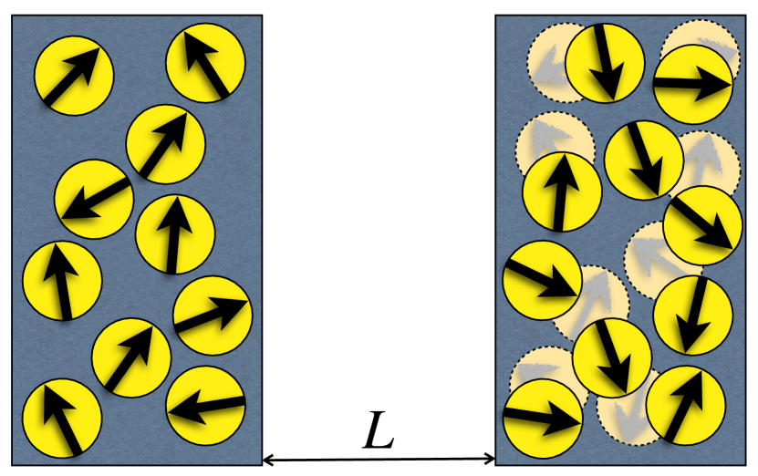
Figure 1: (Color online) Schematic drawing of a classical dipole model of two dielectric half-spaces at separation $L$. The slit region is a vacuum. Fluctuating thermal dipole configurations (shown bold and faint) create a fluctuating thermal Casimir interactions that for large $L$ decay to zero strictly with a probability one.

Connected with the question whether fluctuations in Casimir forces scale thermodynamically, is the intriguing existence of fluctuating forces on isolated bodies, depending on a microscopic cut-off, as such forces should induce movement/diffusion of small inclusions and perhaps also fluctuation-induced drag forces, which have been predicted in a number of quantum drag and thermal tdrag situations. The theoretical results described above point to the existence of regimes, notably in microscopic systems, where fluctuations of measured Casimir forces of both quantum expsq as well as thermal or critical Casimir provenience expscrit , can become large and thus may be experimentally measurable.

In dea2012 a model dielectric was introduced, based on a continuous polarizable dipole field, showing thermal fluctuation forces identical to the zero frequency Matsubara mode van der Waals forces of the standard Lifshitz theory with media of the same dielectric constants. Within this model it is possible to analyze straightforwardly how the van der Waals interaction arises from the correlations between dipoles in opposing slabs and how the van der Waals force evolves temporally when switched on from zero, that is for initially uncorrelated slabs, to its final equilibrium value.

Here we use the very same model to study the fluctuations of the dipole-dipole induced thermal Casimir force in the problem. Because we analyze direct interaction between dipoles, it is clear that as the distance between the two slabs is taken to infinity, the force itself must go to zero. In our model we only take into account the electromagnetic field generated by the dipoles in the slabs and ignore fluctuations of the electromagnetic field due to thermal photons (which cannot be properly included in the classical limit considered here rob1995 ). In this situation therefore, we do not expect a bulk cut-off dependent force fluctuation of the type mentioned above. We find that the average force scales as $\langle f\rangle\sim Ak_{B}T/L^{3}$ while the variance behaves as $\langle f^{2}\rangle_{c}\sim A(k_{B}T)^{2}/L^{4}$ and tends to zero for infinitely distant bodies. We note that the variance obtained behaves like the $L$-dependent part of the variance found in bar2002 .

II Polarizable field model

We consider a classical model of interacting dipoles introduced in dea2012 . Here we have two slabs of material separated by distance $L$ in the direction ${\bf e}_{z}$ and the Hamiltonian for the system is given by

$$H={1\over 2}\int d{\bf x}d{\bf x}^{\prime}\sum_{ij}p_{i}({\bf x})A_{ij}({\bf x},{\bf x}^{\prime};L)p_{j}({\bf x}^{\prime})$$ (1)

where ${\bf p}({\bf x})$ is a local dipole field. The interaction is given by

$$A_{ij}({\bf x},{\bf x}^{\prime}:L)={\delta_{ij}\delta({\bf x}-{\bf x}^{\prime})\over\chi({\bf x})}+D_{ij}({\bf x},{\bf x}^{\prime};L),$$ (2)

where $\chi({\bf x})$ is the local polarizability of the dipole field at the point ${\bf x}$ and $D_{ij}$ is the usual dipole dipole interaction. In slab $S_{i}$ we set $\chi=\chi_{i}$ (for $i=1$ and $2$) and we use a coordinate system such that the points in $S_{1}$ are in the half space $V^{-}:$ $z<0$ and the points in the slab $S_{2}$ are in the half space $V^{+}$: $z>0$. The dipole-dipole interaction is then given by

$$D^{(0)}_{ij}({\bf x}-{\bf x}^{\prime})=\nabla_{i}\nabla^{\prime}_{j}G_{0}({\bf x}-{\bf x}^{\prime})$$ (3)

where $\nabla$ indicates the gradient with respect the the coordinate ${\bf x}$, $\nabla^{\prime}$ the gradient with respect to ${\bf x}^{\prime}$ and $G_{0}$ is the vacuum Green’s function obeying.

$$\epsilon_{0}\nabla^{2}G_{0}({\bf x}-{\bf x}^{\prime})=-\delta({\bf x}-{\bf x^{\prime}}).$$ (4)

With this notation the dipole-dipole interaction is given by

$$D_{ij}({\bf x},{\bf x}^{\prime};L)=\left\{\begin{array}[]{cl}D^{(0)}_{ij}({\bf x}-{\bf x}^{\prime})&{\bf x},{\bf x}^{\prime}\in V^{-},V^{+}\\ D_{ij}^{(0)}({\bf x}-{\bf x}^{\prime}-L{\bf e}_{z})&{\bf x}\in V^{-},{\bf x}^{\prime}\in V^{+}\\ D_{ij}^{(0)}({\bf x}-{\bf x}^{\prime}+L{\bf e}_{z})&{\bf x}^{\prime}\in V^{-},{\bf x}\in V^{+}.\end{array}\right.~{}~{}~{}$$ (5)

Note that we have chosen the slabs to be separated by vacuum, so that there is no bulk pressure associated with the intervening dielectric medium, independent of the plate separation $L$. The thermal Casimir force usually given for such systems equals the plate area multiplied by a disjoining pressure, i.e. the difference between the confined and bulk pressures, which tends asymptotically to zero as the plate separation increases.

For a fixed configuration of dipoles (where both their relative position and orientation are fixed) the instantaneous force on $S_{2}$ is given by

$$f=-{\partial H\over\partial L}=$$

$$-\int_{V^{-}\times V^{+}}\!\!\!\!\!\!\!\!\!\!\!\!\!\!\!d{\bf x}d{\bf x}^{\prime}\sum_{ij}p_{i}({\bf x})\left[{\partial\over\partial L}D_{ij}^{(0)}({\bf x}-{\bf x}^{\prime}-L{\bf e}_{z})\right]p_{j}({\bf x}^{\prime}),~{}~{}~{}~{}~{}~{}~{}$$ (6)

as only the interaction between dipoles in different slabs depends on $L$. Of course each dipole feels both the electric fields from dipoles within the same slab and those in the opposing slab. However, when we infinitesimally displace $S_{2}$, the whole slab moves and each dipole is displaced by the same amount leaving their relative separation and consequently their energy of interaction the same. Let $S_{1}$ denote the half space $z<0$ and $S_{2}$ the half space $z>L$, so that the force is given by

$$\kern-10.0ptf=-\int_{S_{1}\times S_{2}}\!\!\!\!\!\!\!\!\!d{\bf x}d{\bf x}^{\prime}\sum_{ij}p_{i}({\bf x})\left[{\partial\over\partial z^{\prime}}D_{ij}^{(0)}({\bf x}-{\bf x}^{\prime})\right]p_{j}({\bf x}^{\prime}).$$ (7)

This expression for the force has an obvious physical interpretation, which could in fact have been used as a starting point for its definition. The electric field due to the dipoles in $S_{1}$ at the point ${\bf x^{\prime}}$ in $S_{2}$ is given by

$$E_{1j}({\bf x^{\prime}})=-\int_{S_{1}}d{\bf x}\sum_{ij}p_{i}({\bf x})\left[D_{ij}^{(0)}({\bf x}-{\bf x}^{\prime})\right],$$ (8)

and the force in the $z^{\prime}$ direction on a dipole at ${\bf x}^{\prime}$ in the $S_{2}$ due to the dipoles in $S_{1}$ is thus

$$F({\bf x^{\prime}})=-\sum_{j}p_{j}({\bf x^{\prime}}){\partial\over\partial z^{\prime}}E_{1j}({\bf x}^{\prime}),$$ (9)

so Eq. (6) is just $f=\int_{S_{2}}d{\bf x^{\prime}}F({\bf x}^{\prime})$. Now writing the dipole-dipole interaction in terms of the free Green’s function we find

$$f=-\int_{S_{1}\times S_{2}}\!\!\!\!\!\!\!\!\!d{\bf x}d{\bf x}^{\prime}\sum_{ij}p_{i}({\bf x})\left[{\partial\over\partial z^{\prime}}\nabla_{i}\nabla^{\prime}_{j}G_{0}({\bf x}-{\bf x}^{\prime})\right]p_{j}({\bf x}^{\prime}).~{}~{}~{}$$ (10)

It is important to emphasize here that in this model the electric field is a fixed function of the dipole configurations and that we do not consider additional thermal fluctuations of the electromagnetic field.

III Force fluctuations

In principle we can compute moments of the force from Eq. (10), but the calculation can be considerably simplified by considering

$${\partial f\over\partial L}=\int_{S_{1}\times S_{2}}\!\!\!\!\!\!\!\!\!d{\bf x}d{\bf x}^{\prime}\sum_{ij}p_{i}({\bf x})\left[{\partial^{2}\over\partial z^{\prime 2}}\nabla_{i}\nabla^{\prime}_{j}G_{0}({\bf x}-{\bf x}^{\prime})\right]p_{j}({\bf x}^{\prime}),~{}~{}~{}~{}~{}~{}~{}$$ (11)

where, as in Eq. (7), we have simply replaced the derivatives in $L$ by derivatives in $z^{\prime}$. In order to compute the partition function for this system and the correlation function for the dipole field, we first introduce the generating function

$$Z[{\bf u}]=$$

$$\int\prod_{i}d[p_{i}({\bf x})]\exp\left(-\beta H+\!\!\!\int_{S_{1}\cup S_{2}}\!\!\!\!\!\!\!\!\!\!\!\!d{\bf x}\ \sum_{i}u_{i}({\bf x})p_{i}({\bf x})\right),~{}~{}~{}~{}$$ (12)

which can be rewritten introducing an auxiliary field $\phi$ that decouples the dipole-dipole interactions. We can now integrate over the dipole field to obtain

$$\kern-20.0ptZ[{\bf u}] = \int d[\phi({\bf x})]\exp\left(-{\beta\epsilon_{0}\over 2}\int d{\bf x}\ [\nabla\phi]^{2}\right.$$ (13)

$$- \left.{\beta\over 2}\int_{S_{1}\cup S_{2}}\!\!\!\!\!\!\!\!\!d{\bf x}\ \chi({\bf x})(\nabla\phi({\bf x})-{i\over\beta}{\bf u}({\bf x}))^{2}\right),$$

where by setting $\phi=-i\psi$, $\psi$ can be identified as the electrostatic potential. Integrating over the dipole field yields the partition function, while the no source term is immediately recognizable as the zero frequency Matsubara mode or thermal (van der Waals) Casimir interaction of the standard Lifshitz theory par2006

$$Z[{\bf 0}]=\int d[\phi({\bf x})]\exp\left(-{\beta\over 2}\int d{\bf x}\ \epsilon({\bf x})[\nabla\phi]^{2}\right)$$ (14)

with dielectric constants $\epsilon({\bf x})=\epsilon_{0}+\chi_{i}$ when ${\bf x}$ is in $S_{1}$ or $S_{2}$ and $\epsilon({\bf x})=\epsilon_{0}$ for ${\bf x}$ is between the slabs. Written in the form of Eq. (14), but also from the basic model above, it is clear that our model is valid for high temperature dielectric systems, retardation effects are neglected and also no effects due to conduction electrons is present.

In the absence of sources, the average value of the dipole field is $\langle p_{i}({\bf x})\rangle=0$, and its correlation function at non-coinciding points is

$$\langle p_{i}({\bf x})p_{j}({\bf x}^{\prime})\rangle=-{1\over\beta}\chi({\bf x})\chi({\bf x}^{\prime})\nabla_{i}\nabla_{j}^{\prime}G({\bf x},{\bf x}^{\prime}),$$ (15)

where $G$ is the slab geometry Green’s function obeying

$$\nabla\cdot\epsilon({\bf x})\nabla G({\bf x},{\bf x}^{\prime})=-\delta({\bf x}-{\bf x}^{\prime}).$$ (16)

The average force is thermodynamically given via

$$\langle f\rangle=-\langle{\partial H\over\partial L}\rangle={1\over\beta}{\partial\over\partial L}\ln(Z[{\bf 0}]).$$ (17)

To compute the variance of the force one notices that

$${\partial\over\partial L}\langle f\rangle=-\langle{\partial^{2}H\over\partial L^{2}}\rangle+\beta\langle({\partial H\over\partial L})^{2}\rangle_{c}$$ (18)

which can be rearranged to give the Gibbs lemma gibbs type result

$$\langle f^{2}\rangle_{c}=k_{B}T\left[{\partial\over\partial L}\langle f\rangle+\langle{\partial^{2}H\over\partial L^{2}}\rangle\right].$$ (19)

The first term on the right-hand-side is easy to calculate. The second term is obtained from Eqs. (11) and (15) as

$$\beta\langle{\partial^{2}H\over\partial L^{2}}\rangle= -\int_{S_{1}\times S_{2}}\!\!\!\!\!\!\!\!\!d{\bf x}d{\bf x}^{\prime}\sum_{ij}\left[{\partial^{2}\over\partial z^{\prime 2}}\nabla_{i}\nabla^{\prime}_{j}G_{0}({\bf x}-{\bf x}^{\prime})\right]$$ (20)

$$\chi({\bf x})\chi({\bf x}^{\prime})\nabla_{i}\nabla_{j}^{\prime}G({\bf x},{\bf x}^{\prime}).$$

This can be further simplified using the Fourier-Bessel transform of the Green’s functions in the ${\bf r}=(x,y)$ plane to get the remarkably simple formula

$$\beta\langle{\partial^{2}H\over\partial L^{2}}\rangle=-{A\chi_{1}\chi_{2}\over 2\pi}\int dkk^{5}G(k,0,L)G_{0}(k,L).$$ (21)

The lateral Fourier transform of the free Green’s function $G_{0}$ is given by

$$G_{0}(k,z-z^{\prime})={1\over 2\epsilon_{0}k}\exp(-k|z-z^{\prime}|)$$ (22)

while

$$G(k,0,L)={2\epsilon_{0}\exp(-kL)\over k(\epsilon_{0}+\epsilon_{1})(\epsilon_{0}+\epsilon_{2})\left(1-\Delta_{1}\Delta_{2}\exp(-2kL)\right)},$$ (23)

where $\Delta_{i}=(\epsilon_{i}-\epsilon_{0})/(\epsilon_{i}+\epsilon_{0})$. This finally yields

$$\beta\langle{\partial^{2}H\over\partial L^{2}}\rangle=-{3A\Delta_{1}\Delta_{2}\over 8\pi L^{4}}{\rm Li}_{4}(\Delta_{1}\Delta_{2}),$$ (24)

where ${\rm Li}_{s}$ is the polylogarithmic function defined by

$${\rm Li}_{s}(z)=\sum_{n=1}^{\infty}{z^{n}\over n^{s}}$$ (25)

The standard result for the average value of the Casimir force for this system is given by par2006

$$\langle f\rangle=-k_{B}TA{{\rm Li}_{3}(\Delta_{1}\Delta_{2})\over 8\pi L^{3}}.$$ (26)

Putting these results together in Eq. (19) finally yields

$$\langle f^{2}\rangle_{c}={3A(k_{B}T)^{2}\over 8\pi L^{4}}g(\Delta_{1}\Delta_{2})$$ (27)

where $g(z)={\rm Li}_{3}(z)-{\rm Li}_{4}(z)$. The function $g(z)$ is positive for $z\in[0,1]$, so that indeed the variance of the force fluctuations is everywhere positive. We see that the scaling of the fluctuations agrees with the $L$ dependent part in bar2002 , but contains no bulk term dependent on an ultra-violet cut-off.

The ratio of the variance to the squared average force is then given by

$$Q={\langle f^{2}\rangle_{c}\over\langle f\rangle^{2}}={24\pi L^{2}\over A}h(z)$$ (28)

where $h(z)=g(z)/{\rm Li}^{2}_{3}(z)$ and $h(z)$ attains its maximum value $0.08286$ at $z=1$. Note the results are symmetric under the interchange of the labels $1$ and $2$ and thus the average force on each slab is equal and opposite and the force fluctuations on both slabs are the same. This has to be the case, as from the definition of the unaveraged force it is clear that the forces exerted on each of the slabs are symmetric.

IV conclusions

We analyzed a simple, classical dipole model, that leads to thermal van der Waals interactions with the average force predicted by the standard Lifshitz theory. In this classical dipole model the force at large separations not only goes to zero on the average, but much more stringently with probability one. The ratio of the variance to the squared average force, Eq. (28), furthermore gives a fingerprint of the classical thermal van de Waals interaction, differentiating it from possible parasitic effects and stray interactions, plaguing experiments in realistic systems Disorder .

In our dipole model there is no divergent cut-off dependent bulk contribution to the average force. The fact that no other length scale appears means that the functional form of the force variance in Eq. (27) can be predicted solely on the grounds of dimensional analysis and by assuming the thermodynamic scaling, i.e. $\Delta f\sim\sqrt{A}$ for the fluctuations as a function of the area of the plates. The so obtained thermodynamic scaling is in agreement with a number of studies of fluctuations of Casimir forces in both thermal and quantum systems bar1991 ; ebe1991 ; bar2002 . The results of bar2002 are for thermally fluctuating fields, as here, but find a microscopic cut-off depend force fluctuations at infinite plate separation. Nevertheless the average force has the same behavior in both models. This difference comes naturally from an underlying microscopic definition of the model. In our model the electrostatic fields are generated by the dipoles themselves, being solutions of the Poisson equation for the given dipole distribution. The fields so generated cannot generate self-forces on isolated objects, hence as the two slabs are separated the total force on each slab decays to zero and by consequence so does its mean and variance. In the model of bar2002 (and indeed its quantum counterparts bar1991 ; ebe1991 ), the fluctuating field exists throughout space and objects immersed in the field are not its sources. The objects immersed in the field however modify its fluctuations by the imposition of boundary conditions. Crucially however, the fluctuating field exists in the presence of a single object and hence can exert a force, albeit of mean zero, on the object. Intriguingly, the nature of force fluctuations may therefore be relevant to the long standing debate (see cug12 for a recent discussion) as to the physical interpretation of the Casimir effect in terms of a shift in zero point energy (field effect) or as a van der Waals effect (due to sources). It should be noted that fluctuations of the force acting on a single particle is compatible with the drag predicted on isolated moving objects coupled to a thermalized fluctuating field drag ; tdrag .

Normally in electrostatics forces are evaluated by using the stress tensor lan75 that follows from equations of the form of Eq. (9), in order to compute forces generated by electric fields on charges and/or dipoles. The usual stress tensor given for dielectric systems depends on the local dielectric constant lan75 which is already an object derived from thermodynamic averaging, relating the average local polarization field to the local electric field. This means that the validity of the use of the preaveraged stress tensor to compute fluctuations of forces in these types of models is not obvious. The stress tensor before averaging is a fundamental object derived from the force exerted on charges by the electric field. It is indeed this stress tensor that should be used to compute force fluctuations. However, in many coarse grained theories used to describe fluctuating systems, dynamical variables, which are equivalent to charges or dipoles in electrostatic language, have been integrated out in formulating the theory and it is thus not always obvious that they contain sufficient physical information to yield correct predictions for force fluctuations.

References

- (1) M. Kardar and R. Golestanian, Rev. Mod. Phys. 71, 1233 (1999); K.A. Milton, The Casimir Effect: Physical Manifestations of Zero-Point Energy (World Scientific, Singapore) (2001); M. Bordag , G.L. Klimchitskaya , U. Mohideen , and V.M. Mostepanenko, Advances in the Casimir Effect (Oxford University Press, Oxford) (2009); M.E. Fisher and P.G. de Gennes, C. R. Acad. Sci. Paris B 287, 207 (1976)
- (2) A. Naji, D.S. Dean, J. Sarabadani, R.R. Horgan, and R. Podgornik, Phys. Rev. Lett.104 060601 (2010).
- (3) G. Barton, J. Phys. A: Math. Gen. 24 991 (1991). G. Barton, J. Phys. A: Math. Gen. 24 5553 (1991).
- (4) C. Eberlein, J. Phys. A: Math. Gen. 25 3015 (1991).
- (5) M. T. Jaekel and S. Reynaud, Quantum Opt. 4, 39 (1992).
- (6) C.-H. Wu and L. H. Ford, Phys. Rev. D 64, 045010 (2001).
- (7) D. Robaschik and E. Wieczorek, Phys. Rev. D 52, 2341 (1995).
- (8) C.-H. Wu, C.-I. Kuo, and L. H. Ford, Phys. Rev. A 65, 062102 (2002).
- (9) R. Messina and R. Passante, Phys. Rev. A 76, 032107 (2007).
- (10) D. Bartolo, A. Ajdari, J.-B. Fournier and R. Golestanian, Phys. Rev. Lett. 89, 230601, (2002).
- (11) A.-F. Bitbol, P.G. Dommersnes and J.-B. Fournier, Phys. Rev. E 81 (2010).
- (12) P. Rodriguez-Lopez, R. Brito and R. Soto, Europhys. Lett. 96 50008 (2011).
- (13) V. Mkrtchian, V.A. Parsegian, R. Podgornik and W.M. Saslow, Phys. Rev. Lett. 91, 220801 (2003); G.E. Astrakharchik and L.P. Pitaevskii, Phys. Rev. A 70, 013608 (2004); D.C.Roberts and Y. Pomeau, Phys. Rev, Lett. 95, 145303 (2005); A.G. Sykes, M.J. Davis and D.C. Roberts, Phys. Rev. Lett. 103, 085302 (2009); J.B. Pendry, New J. Phys. 12 033028 (2010);
- (14) V. Démery and D.S. Dean, Phys. Rev. Lett. 104, 080601, (2010); V. Démery and D.S. Dean, Eur. Phys. J E 32, 377 (2010); V. Démery and D.S. Dean, Phys. Rev. E 84, 010103(R) (2011).
- (15) G. Bressi, G. Carugno, R. Onofrio, and G. Ruoso, Phys. Rev. Lett.88, 041804 (2002); S. K. Lamoreaux, Phys. Rev. Lett. 78, 5 (1997); A. Lambrecht and S. Reynaud, Phys. Rev. Lett. 84 , 5672 (2000); U. Mohideen and A. Roy, Phys. Rev. Lett 81 4549 (1998).
- (16) C. Hertlein, L. Helden, A. Gambassi, S. Dietrich and C. Bechinger, Nature 451, 172 (2008); A. Gambassi, A. Maciolek , C. Hertlein, U. Nellen, L. Helden, C. Bechinger and S. Dietrich, Phys. Rev. E 80, 061143 (2009); D. Bonn, J. Otwinowskim S. Sacanna, H. Guo, G. Wedgam and P. Schall, Phys. Rev. Lett. 103, 156101 (2009).
- (17) D.S. Dean, V. Démery, V.A. Parsegian and R. Podgornik, Phys. Rev. E 85, 031108 (2012).
- (18) J.W. Gibbs, Elementary principles in statistical mechanics, New York, (C. Scribner) (1902).
- (19) V. A. Parsegian, Van der Waals Forces, Cambridge (Cambridge) (2006).
- (20) J. Cugnon, Few-Body Syst. 53, 181 (2012).
- (21) L. D. Landau and E.M. Lifshitz, The Classical Theory of Fields (Pergamon, Oxford, England, 1975), 4th ed.