Rotational Projection Statistics for 3D Local Surface Description and Object Recognition

Abstract

Recognizing 3D objects in the presence of noise, varying mesh resolution, occlusion and clutter is a very challenging task. This paper presents a novel method named Rotational Projection Statistics (RoPS). It has three major modules: Local Reference Frame (LRF) definition, RoPS feature description and 3D object recognition. We propose a novel technique to define the LRF by calculating the scatter matrix of all points lying on the local surface. RoPS feature descriptors are obtained by rotationally projecting the neighboring points of a feature point onto 2D planes and calculating a set of statistics (including low-order central moments and entropy) of the distribution of these projected points. Using the proposed LRF and RoPS descriptor, we present a hierarchical 3D object recognition algorithm. The performance of the proposed LRF, RoPS descriptor and object recognition algorithm was rigorously tested on a number of popular and publicly available datasets. Our proposed techniques exhibited superior performance compared to existing techniques. We also showed that our method is robust with respect to noise and varying mesh resolution. Our RoPS based algorithm achieved recognition rates of 100%, 98.9%, 95.4% and 96.0% respectively when tested on the Bologna, UWA, Queen’s and Ca’ Foscari Venezia Datasets.

1 Introduction

Object recognition is an active research area in computer vision with numerous applications including navigation, surveillance, automation, biometrics, surgery and education (Guo et al., 2013c; Johnson and Hebert, 1999; Lei et al., 2013; Tombari et al., 2010). The aim of object recognition is to correctly identify the objects that are present in a scene and recover their poses (i.e., position and orientation) (Mian et al., 2006b). Beyond object recognition from 2D images (Brown and Lowe, 2003; Lowe, 2004; Mikolajczyk and Schmid, 2004), 3D object recognition has been extensively investigated during the last two decades due to the availability of low cost scanners and high speed computing devices (Mamic and Bennamoun, 2002). However, recognizing objects from range images in the presence of noise, varying mesh resolution, occlusion and clutter is still a challenging task.

Existing algorithms for 3D object recognition can broadly be classified into two categories, i.e., global feature based and local feature based algorithms (Bayramoglu and Alatan, 2010; Castellani et al., 2008). The global feature based algorithms construct a set of features which encode the geometric properties of the entire 3D object. Examples of these algorithms include the geometric 3D moments (Paquet et al., 2000), shape distribution (Osada et al., 2002) and spherical harmonics (Funkhouser et al., 2003). However, these algorithms require complete 3D models and are therefore sensitive to occlusion and clutter (Bayramoglu and Alatan, 2010). In contrast, the local feature based algorithms define a set of features which encode the characteristics of the local neighborhood of feature points. The local feature based algorithms are robust to occlusion and clutter. They are therefore even suitable to recognize partially visible objects in a cluttered scene (Petrelli and Di Stefano, 2011).

A number of local feature based 3D object recognition algorithms have been proposed in the literature, including point signature based (Chua and Jarvis, 1997), spin image based (Johnson and Hebert, 1999), tensor based (Mian et al., 2006b) and Exponential Map (EM) based (Bariya et al., 2012) algorithms. Most of these algorithms follow a paradigm that has three phases, i.e., feature matching, hypothesis generation and verification, and pose refinement (Taati and Greenspan, 2011). Among these phases, feature matching plays a critical role since it directly affects the effectiveness and efficiency of the two subsequent phases (Taati and Greenspan, 2011).

Descriptiveness and robustness of a feature descriptor are crucial for accurate feature matching (Bariya and Nishino, 2010). The feature descriptors should be highly descriptive to ensure an accurate and efficient object recognition. That is because the accuracy of feature matching directly influences the quality of the estimated transformation which is used to align the model to the scene, as well as the computational time required for verification and refinement (Taati and Greenspan, 2011). Moreover, the feature descriptors should be robust to a set of nuisances, including noise, varying mesh resolution, clutter, occlusion, holes and topology changes (Bronstein et al., 2010a; Boyer et al., 2011).

A number of local feature descriptors exist in literature (Section 2.1). These descriptors can be divided into two broad categories based on whether they use a Local Reference Frame (LRF) or not. Feature descriptors without any LRF use a histogram or the statistics of the local geometric information (e.g., normal, curvature) to form a feature descriptor (Section 2.1.1). Examples of this category include surface signature (Yamany and Farag, 2002), Local Surface Patch (LSP) (Chen and Bhanu, 2007) and THRIFT (Flint et al., 2007). In contrast, feature descriptors with LRF encode the spatial distribution and/or geometric information of the neighboring points with respect to the defined LRF (Section 2.1.2). Examples include spin image (Johnson and Hebert, 1999), Intrinsic Shape Signatures (ISS) (Zhong, 2009) and MeshHOG (Zaharescu et al., 2012). However, most of the existing feature descriptors still suffer from either low descriptiveness or weak robustness (Bariya et al., 2012).

In this paper we present a highly descriptive and robust feature descriptor together with an efficient 3D object recognition algorithm. This paper first proposes a unique, repeatable and robust LRF for both local feature description and object recognition (Section 3). The LRF is constructed by performing an eigenvalue decomposition on the scatter matrix of all the points lying on the local surface together with a sign disambiguation technique. A novel feature descriptor, namely Rotational Projection Statistics (RoPS), is then presented (Section 4). RoPS exhibits both high discriminative power and strong robustness to noise, varying mesh resolution and a set of deformations. The RoPS feature descriptor is generated by rotationally projecting the neighboring points onto three local coordinate planes and calculating several statistics (e.g, central moment and entropy) of the distribution matrices of the projected points. Finally, this paper presents a novel hierarchical 3D object recognition algorithm based on the proposed LRF and RoPS feature descriptor (Section 6). Comparative experiments on four popular datasets were performed to demonstrate the superiority of the proposed method (Section 7).

The rest of this paper is organized as follows. Section 2 provides a brief literature review of local surface feature descriptors and 3D object recognition algorithms. Section 3 introduces a novel technique for LRF definition. Section 4 describes our proposed RoPS method for local surface feature description. Section 5 presents the evaluation results of the RoPS descriptor on two datasets. Section 6 introduces a RoPS based hierarchical algorithm for 3D object recognition. Section 7 presents the results and analysis of our 3D object recognition experiments on four datasets. Section 8 concludes this paper.

2 Related Work

This section presents a brief overview of the existing main methods for local surface feature description and local feature based 3D object recognition.

2.1 Local Surface Feature Description

2.1.1 Features without LRF

Stein and Medioni (1992) proposed a splash feature by recording the relationship between the normals of the geodesic neighboring points and the feature point. This relationship is then encoded into a 3D vector and finally transformed into curvatures and torsion angles. Hetzel et al. (2001) constructed a set of features by generating histograms using depth values, surface normals, shape indices and their combinations. Results show that the surface normal and shape index exhibit high discrimination capabilities. Yamany and Farag (2002) introduced a surface signature by encoding the surface curvature information into a 2D histogram. This method can be used to estimate scaling transformations as well as recognizing objects in 3D scenes. Chen and Bhanu (2007) proposed a LSP feature that encodes the shape indices and normal deviations of the neighboring points. Flint et al. (2008) introduced a THRIFT feature by calculating a weighted histogram of the deviation angles between the normals of the neighboring points and the feature point. Taati et al. (2007) considered the selection of a good local surface feature for 3D object recognition as an optimization problem and proposed a set of Variable-Dimensional Local Shape Descriptors (VD-LSD). However, the process of selecting an optimized subset of VD-LSDs for a specific object is very time consuming (Taati and Greenspan, 2011). Kokkinos et al. (2012) proposed a generalization of 2D shape context feature (Belongie et al., 2002) to curved surfaces, namely Intrinsic Shape Context (ISC). The ISC is a meta-descriptor which can be applied to any photometric or geometric field defined on a surface.

Without LRF, most of these methods generate a feature descriptor by accumulating certain geometric attributes (e.g., normal, curvature) into a histogram. Since most of the 3D spatial information is discarded during the process of histogramming, the descriptiveness of the features without LRF is limited (Tombari et al., 2010).

2.1.2 Features with LRF

Chua and Jarvis (1997) proposed a point signature by using the distances from the neighboring points to their corresponding projections on a fitted plane. One merit of the point signature is that no surface derivative is required. One of its limitations relate to the fact that the reference direction may not be unique. It is also sensitive to mesh resolution (Mian et al., 2010). Johnson and Hebert (1998) used the surface normal as a reference axis and proposed a spin image representation by spinning a 2D image about the normal of a feature point and summing up the number of points falling into the bins of that image. The spin image is one of the most cited methods. But its descriptiveness is relatively low and it is also sensitive to mesh resolution (Zhong, 2009). Frome et al. (2004) also used the normal vector as a reference axis and generated a 3D Shape Context (3DSC) by counting the weighted number of points falling in the neighboring 3D spherical space. However, a reference axis is not a complete reference frame and there is an uncertainty in the rotation around the normal (Petrelli and Di Stefano, 2011).

Sun and Abidi (2001) introduced an LRF by using the normal of a feature point and an arbitrarily chosen neighboring point. Based on the LRF, they proposed a descriptor named point’s fingerprint by projecting the geodesic circles onto the tangent plane. It was reported that their approach outperforms the 2D histogram based methods. One major limitation of this method is that their LRF is not unique (Tombari et al., 2010). Mian et al. (2006b) proposed a tensor representation by defining an LRF for a pair of oriented points and encoding the intersected surface area into a multidimensional table. This representation is robust to noise, occlusion and clutter. However, a pair of points are required to define an LRF, which causes a combinatorial explosion (Zhong, 2009). Novatnack and Nishino (2008) used the surface normal and a projected eigenvector on the tangent plane to define an LRF. They proposed an EM descriptor by encoding the surface normals of the neighboring points into a 2D domain. The effectiveness of exploiting geometric scale variability in the EM descriptor has been demonstrated. Zhong (2009) introduced an LRF by calculating the eigenvectors of the scatter matrix of the neighboring points of a feature point, and proposed an ISS feature by recording the point distribution in the spherical angular space. Since the sign of the LRF is not defined unambiguously, four feature descriptors can be generated from a single feature point. Mian et al. (2010) proposed a keypoint detection method and used a similar LRF to Zhong (2009) for their feature description. Tombari et al. (2010) analyzed the strong impact of LRF on the performance of feature descriptors and introduced a unique and unambiguous LRF by performing an eigenvalue decomposition on the scatter matrix of the neighboring points and using a sign disambiguation technique. Based on the proposed LRF, they introduced a feature descriptor called Signature of Histograms of OrienTations (SHOT). SHOT is very robust to noise, but sensitive to mesh resolution variation. Petrelli and Di Stefano (2011) proposed a novel LRF which aimed to estimate a repeatable LRF at the border of a range image. Zaharescu et al. (2012) proposed a MeshHOG feature by first projecting the gradient vectors onto three planes defined by an LRF and then calculating a two-level histogram of these vectors.

However, none of the existing LRF definition techniques is simultaneously unique, unambiguous, and robust to noise and mesh resolution. Besides, most of the existing feature descriptors suffer from a number of limitations, including a low robustness and discriminating power (Bariya et al., 2012).

2.2 3D Object Recognition

Most of the existing algorithms for local feature based 3D object recognition follow a three-phase paradigm including feature matching, hypothesis generation and verification, and pose refinement (Taati and Greenspan, 2011).

Stein and Medioni (1992) used the splash features to represent the objects and generated hypotheses by using a set of triplets of feature correspondences. These hypotheses are then grouped into clusters using geometric constraints. They are finally verified through a least square calculation. Chua and Jarvis (1997) used point signatures of a scene to match them against those of their models. The rigid transformation between the scene and a candidate model was then calculated using three pairs of corresponding points. Its ability to recognize objects in both single-object and multi-object scenes has been demonstrated. However, verifying each triplet of feature correspondences is very time consuming. Johnson and Hebert (1999) generated point correspondences by matching the spin images of the scene with the spin images of the models. These point correspondences are first grouped using geometric consistency. The groups are then used to calculate rigid transformations, which are finally be verified. This algorithm is robust to clutter and occlusion, and capable to recognize objects in complicated real scenes. Yamany and Farag (2002) used surface signatures as feature descriptors and adopted a similar strategy to Johnson and Hebert (1999) for object recognition. Mian et al. (2006b) obtained feature correspondences and model hypothesis by matching the tensor representations of the scene with those of the models. The hypothesis model is then transformed to the scene and finally verified using the Iterative Closest Point (ICP) algorithm (Besl and McKay, 1992). Experimental results revealed that it is superior in terms of recognition rate and efficiency compared to the spin image based algorithm. Mian et al. (2010) also developed a 3D object recognition algorithm based on keypoint matching. This algorithm can be used to recognize objects at different and unknown scales. Taati and Greenspan (2011) developed a 3D object recognition algorithm based on their proposed VD-LSD feature descriptors. The optimal VD-LSD descriptor is selected based on the geometry of the objects and the characteristics of the range sensors. Bariya et al. (2012) introduced a 3D object recognition algorithm based on the EM feature descriptor and a constrained interpretation tree.

There are some algorithms in the literature which do not follow the aforementioned three-phase paradigm. For example, Frome et al. (2004) performed 3D object recognition using the sum of the distances between the scene features (i.e. 3DSC) and their corresponding model features. This algorithm is efficient. However, it is not able to segment the recognized object from a scene, and its effectiveness on real data has not been demonstrated. Shang and Greenspan (2010) proposed a Potential Well Space Embedding (PWSE) algorithm for real-time 3D object recognition in sparse range images. It cannot however handle clutter and therefore requires the objects to be segmented a priori from the scene.

None of the existing object recognition algorithms has explicitly explored the use of LRF to boost the performance of the recognition. Moreover, most of these algorithms require three pairs of feature correspondences to establish a transformation between a model and a scene. This not only increases the run time due to the combinatorial explosion of the matching pairs, but also decreases the precision of the estimated transformation (since the chance to find three correct feature correspondences is much lower compared to finding only one correct correspondence).

2.3 Paper Contributions

This paper is an extended version of (Guo et al., 2013a, b). It has three major contributions, which are summarized as follows.

i) We introduce a unique, unambiguous and robust 3D LRF using all the points lying on the local surface rather than just the mesh vertices. Therefore, our proposed LRF is more robust to noise and varying mesh resolution. We also use a novel sign disambiguation technique, our proposed LRF is therefore unique and unambiguous. This LRF offers a solid foundation for effective and robust feature description and object recognition.

ii) We introduce a highly descriptive and robust RoPS feature descriptor. RoPS is generated by rotationally projecting the neighboring points onto three coordinate planes and encoding the rich information of the point distribution into a set of statistics. The proposed RoPS descriptor has been evaluated on two datasets. Experimental results show that RoPS achieved a high power of descriptiveness. It is shown to be robust to a number of deformations including noise, varying mesh resolution, rotation, holes and topology changes. (see Section 5 for details) .

iii) We introduce an efficient hierarchical 3D object recognition algorithm based on the LRF and RoPS feature descriptor. One major advantage of our algorithm is, a single correct feature correspondence is sufficient for object recognition. Moreover, by integrating our robust LRF, the proposed object recognition algorithm can work with any of the existing feature descriptors (e.g., spin image) in the literature. Rigorous evaluations of the proposed 3D object recognition algorithm were conducted on four different popular datasets. Experimental results show that our algorithm achieved high recognition rates, good efficiency and strong robustness to different nuisances. It consistently resulted in the best recognition results on the four datasets.

3 Local Reference Frame

A unique, repeatable and robust LRF is important for both effective and efficient feature description and 3D object recognition. Advantages of such an LRF are many fold. First, the repeatability of an LRF directly affects the descriptiveness and robustness of the feature descriptor, i.e., an LRF with a low repeatability will result in a poor performance of feature matching (Petrelli and Di Stefano, 2011). Second, compared with the methods which associate multiple descriptors to a single feature point (e.g., ISS (Zhong, 2009)), a unique LRF can help to improve both the precision and the efficiency of feature matching (Tombari et al., 2010). Third, a robust 3D LRF helps to boost the performance of 3D object recognition.

We propose a novel LRF by fully employing the point localization information of the local surface. The three axes for the LRF are determined by performing an eigenvalue decomposition on the scatter matrix of all points lying on the local surface. The sign of each axis is disambiguated by aligning the direction to the majority of the point scatter.

3.1 Coordinate Axis Construction

Given a feature point $\boldsymbol{p}$ and a support radius $r$, the local surface mesh $S$ which contains $N$ triangles and $M$ vertices, is cropped from the range image using a sphere of radius $r$ centered at $\boldsymbol{p}$. For the $i$th triangle with vertices $\boldsymbol{p}_{i1}$, $\boldsymbol{p}_{i2}$ and $\boldsymbol{p}_{i3}$, a point lying within the triangle can be represented as:

$$\boldsymbol{p}_{i}\left(s,t\right)=\boldsymbol{p}_{i1}+s(\boldsymbol{p}_{i2}-\boldsymbol{p}_{i1})+t\left(\boldsymbol{p}_{i3}-\boldsymbol{p}_{i1}\right),$$ (1)

where $0\leq s,t\leq 1$, and $s+t\leq 1$, as illustrated in Fig. 1.

Figure 1: An illustration of a triangle mesh and a point lying on the surface. An arbitrary point within a triangle can be represented by the triangle’s vertices.

(a) Armadillo

(b) Asia Dragon

(c) Bunny

(d) Dragon

(e) Happy Buddha

(f) Thai Statue

Figure 2: The six models of the Tuning Dataset.

The scatter matrix $\mathbf{C}_{i}$ of all the points lying within the $i$th triangle can be calculated as:

$$\mathbf{C}_{i}=\frac{\int_{0}^{1}\int_{0}^{1-s}\left(\boldsymbol{p}_{i}\left(s,t\right)-\boldsymbol{p}\right)\left(\boldsymbol{p}_{i}\left(s,t\right)-\boldsymbol{p}\right)^{\textrm{T}}dtds}{\int_{0}^{1}\int_{0}^{1-s}dtds}.$$ (2)

Using Eq. 1, the scatter matrix $\mathbf{C}_{i}$ be can expressed as:

$$\mathbf{C}_{i} = \frac{1}{12}\sum_{j=1}^{3}\sum_{k=1}^{3}\left(\boldsymbol{p}_{ij}-\boldsymbol{p}\right)\left(\boldsymbol{p}_{ik}-\boldsymbol{p}\right)^{\textrm{T}}$$ (3)

$$+\frac{1}{12}\sum_{j=1}^{3}\left(\boldsymbol{p}_{ij}-\boldsymbol{p}\right)\left(\boldsymbol{p}_{ij}-\boldsymbol{p}\right)^{\textrm{T}}.$$

The overall scatter matrix $\mathbf{C}$ of the local surface S is calculated as the weighted sum of the scatter matrices of all the triangles, that is:

$$\mathbf{C}=\sum_{i=1}^{N}w_{i1}w_{i2}\mathbf{C}_{i},$$ (4)

where $N$ is the number of triangles in the local surface $S$. Here, $w_{i1}$ is the ratio between the area of the $i$th triangle and the total area of the local surface $S$, that is:

$$w_{i1}=\frac{\left|\left(\boldsymbol{p}_{i2}-\boldsymbol{p}_{i1}\right)\times\left(\boldsymbol{p}_{i3}-\boldsymbol{p}_{i1}\right)\right|}{\sum_{i=1}^{N}\left|\left(\boldsymbol{p}_{i2}-\boldsymbol{p}_{i1}\right)\times\left(\boldsymbol{p}_{i3}-\boldsymbol{p}_{i1}\right)\right|},$$ (5)

where $\times$ denotes the cross product.

$w_{i2}$ is a weight that is related to the distance from the feature point to the centroid of the $i$th triangle, that is:

$$w_{i2}=\left(r-\left|\boldsymbol{p}-\frac{\boldsymbol{p}_{i1}+\boldsymbol{p}_{i2}+\boldsymbol{p}_{i3}}{3}\right|\right)^{2}.$$ (6)

Note that, the first weight $w_{i1}$ is expected to improve the robustness of LRF to varying mesh resolutions, since a compensation with respect to the triangle area is incorporated through this weighting. The second weight $w_{i2}$ is expected to improve the robustness of LRF to occlusion and clutter, since distant points will contribute less to the overall scatter matrix.

We then perform an eigenvalue decomposition on the overall scatter matrix $\mathbf{C}$, that is:

$$\mathbf{C}\mathbf{V}=\mathbf{EV},$$ (7)

where $\mathbf{E}$ is a diagonal matrix of the eigenvalues $\left\{\lambda_{1},\lambda_{2},\lambda_{3}\right\}$ of the matrix $\mathbf{C}$, and $\mathbf{V}$ contains three orthogonal eigenvectors $\left\{\boldsymbol{v}_{1},\boldsymbol{v}_{2},\boldsymbol{v}_{3}\right\}$ that are in the order of decreasing magnitude of their associated eigenvalues. The three eigenvectors offer a basis for LRF definition. However, the signs of these vectors are numerical accidents and are not repeatable between different trials even on the same surface (Bro et al., 2008; Tombari et al., 2010). We therefore propose a novel sign disambiguation technique which is described in the next subsection.

It is worth noting that, although some existing techniques also use the idea of eigenvalue decomposition to construct the LRF (e.g., (Mian et al., 2010; Tombari et al., 2010; Zhong, 2009)), they calculate the scatter matrix using just the mesh vertices. Instead, our technique employs all the points in the local surface and, is therefore more robust compared to exiting techniques (as demonstrated in Section 3.3).

3.2 Sign Disambiguation

In order to eliminate the sign ambiguity of the LRF, each eigenvector should point in the major direction of the scatter vectors (which start from the feature point and point in the direction of the points lying on the local surface). Therefore, the sign of each eigenvector is determined from the sign of the inner product of the eigenvector and the scatter vectors. Specifically, the unambiguous vector $\widetilde{\boldsymbol{v}_{1}}$ is defined as:

$$\widetilde{\boldsymbol{v}_{1}}=\boldsymbol{v}_{1}\cdot\textrm{sign}\left(h\right),$$ (8)

where $\mathrm{sign\left(\cdot\right)}$ denotes the signum function that extracts the sign of a real number, and $h$ is calculated as:

$$h = \sum_{i=1}^{N}w_{i1}w_{i2}\left(\int_{0}^{1}\int_{0}^{1-s}\left(\boldsymbol{p}_{i}\left(s,t\right)-\boldsymbol{p}\right)\boldsymbol{v}_{1}dtds\right)$$ (9)

$$= \sum_{i=1}^{N}w_{i1}w_{i2}\left(\frac{1}{6}\sum_{j=1}^{3}\left(\boldsymbol{p}_{ij}-\boldsymbol{p}\right)\boldsymbol{v}_{1}\right).$$

Similarly, the unambiguous vector $\widetilde{\boldsymbol{v}_{3}}$ is defined as:

$$\widetilde{\boldsymbol{v}_{3}}=\boldsymbol{v}_{3}\cdot\textrm{sign}\left(\sum_{i=1}^{N}w_{i1}w_{i2}\left(\frac{1}{6}\sum_{j=1}^{3}\left(\boldsymbol{p}_{ij}-\boldsymbol{p}\right)\boldsymbol{v}_{3}\right)\right).$$ (10)

Given two unambiguous vectors $\widetilde{\boldsymbol{v}_{1}}$ and $\widetilde{\boldsymbol{v}_{3}}$, $\widetilde{\boldsymbol{v}_{2}}$ is defined as $\widetilde{\boldsymbol{v}_{3}}\times\widetilde{\boldsymbol{v}_{1}}$. Therefore, a unique and unambiguous 3D LRF for feature point $\boldsymbol{p}$ is finally defined. Here, $\boldsymbol{p}$ is the origin, and $\widetilde{\boldsymbol{v}_{1}}$, $\widetilde{\boldsymbol{v}_{2}}$ and $\widetilde{\boldsymbol{v}_{3}}$ are the $x$, $y$ and $z$ axes respectively. With this LRF, a unique, pose invariant and highly discriminative local feature descriptor can now be generated.

3.3 Performance of the Proposed LRF

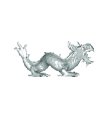
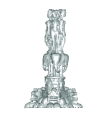
To evaluate the repeatability and robustness of our proposed LRF, we calculated the LRF errors between the corresponding points in the scenes and models. The six models (i.e., “Armadillo”, “Asia Dragon”, “Bunny”, “Dragon”, “Happy Buddha” and “Thai Statue”) used in this experiment were taken from the Stanford 3D Scanning Repository (Curless and Levoy, 1996). They are shown in Fig. 2. The six scenes were created by resampling the models down to $\nicefrac{{1}}{{2}}$ of their original mesh resolution and then adding Gaussian noise with a standard deviation of 0.1 mesh resolution (mr) to the data. We refer to this dataset as the “Tuning Dataset” in the rest of this paper.

We randomly selected 1000 points in each model and we refer to these points as feature points. We then obtained the corresponding points in the scene by searching the points with the smallest distances to the feature points in the model. For each point pair $\left(\boldsymbol{p}_{Si},\boldsymbol{p}_{Mi}\right)$, we calculated the LRFs for both points, denoted as $\mathbf{L}_{Si}$ and $\mathbf{L}_{Mi}$, respectively. Using the similar criterion as in (Mian et al., 2006a), the error between two LRFs of the $i$th point pair can be calculated by:

$$\epsilon_{i}=\arccos\left(\frac{\textrm{trace}\left(\mathbf{L}_{Si}\mathbf{L}_{Mi}^{-1}\right)-1}{2}\right)\frac{180}{\pi},$$ (11)

where $\epsilon_{i}$ represents the amount of rotation error between two LRFs and is zero in the case of no error.

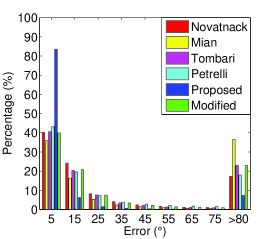
Our proposed LRF technique was tested on the Tuning Dataset with comparison to several existing techniques, e.g., proposed by Novatnack and Nishino (2008), Mian et al. (2010), Tombari et al. (2010), and Petrelli and Di Stefano (2011). We tested each LRF technique five times by randomly selecting 1000 different point pairs each time. The overall LRF errors of each technique are shown in Fig. 3 as a histogram. Ideally, all of the LRF errors should lie around the zero value (in the first bin of the histogram). It is clear that our proposed technique performed best, with 83.5% of the point pairs having LRF errors less than 10 degrees. Whereas the second best one (i.e., proposed by Petrelli and Di Stefano (2011)) secured only 43.2% of the point pairs with LRF errors less than 10 degrees. Other techniques only had around 40% point pairs with LRF errors less than 10 degrees. These results clearly indicate that our proposed LRF is more repeatable and more robust than the state-of-the-art in the presence of noise and mesh resolution variation.

In order to further assess the influence of a weighting strategy, we used a distance weight $w_{i3}=r-\left|\boldsymbol{p}-\frac{\boldsymbol{p}_{i1}+\boldsymbol{p}_{i2}+\boldsymbol{p}_{i3}}{3}\right|$ (following the approach of (Tombari et al., 2010)) to replace the weights $w_{i1}$ and $w_{i2}$ in Equations 4, 9 and 10, resulting in a modified LRF. The histogram of LRF errors of the modified technique is shown in Fig. 3. The performance of the modified LRF decreased significantly compared to the original proposed LRF. This observation reveals that the weighting strategy using both quadratic distance weight $w_{i2}$ and area weight $w_{i1}$ produced more robust results compared to those using only a linear distance weight $w_{i3}$.

Fig. 3 shows that part of the LRF errors of each technique are larger than 80 degrees. This is mainly due to the presence of local symmetrical surfaces (e.g., flat or spherical surfaces) in the scenes. For a local symmetrical surface, there is an inherent sign ambiguity of its LRF because the distribution of points is almost the same in all directions. In order to deal with this case, we adopt a feature point selection technique which uses the ratio of eigenvalues to avoid local symmetrical surfaces (see Section 6.2).

Once an LRF is determined, the next step is to define a local surface descriptor. In the next section, we propose a novel RoPS descriptor.

4 Local Surface Description

A local surface descriptor needs to be invariant to rotation and robust to noise, varying mesh resolution, occlusion, clutter and other nuisances. In this section, we propose a novel local surface feature descriptor namely RoPS by performing local surface rotation, neighboring points projection and statistics calculation.

4.1 RoPS Feature Descriptor

An illustrative example of the overall RoPS method is given in Fig. 4. From a range image/model, a local surface is selected for a feature point $\boldsymbol{p}$ given a support radius $r$. Figures 4(a) and (b) respectively show a model and a local surface. We already have defined the LRF for $\boldsymbol{p}$ and the vertices of the triangles in the local surface $S$ constitute a pointcloud $\mathbf{Q}=\left\{\boldsymbol{q}_{1},\boldsymbol{q}_{2},\ldots,\boldsymbol{q}_{M}\right\}$. The pointcloud $\mathbf{Q}=\left\{\boldsymbol{q}_{1},\boldsymbol{q}_{2},\ldots,\boldsymbol{q}_{M}\right\}$ is then transformed with respect to the LRF in order to achieve rotation invariance, resulting in a transformed pointcloud $\mathbf{Q}^{\prime}=\left\{\boldsymbol{q}_{1}^{\prime},\boldsymbol{q}_{2}^{\prime},\ldots,\boldsymbol{q}_{M}^{\prime}\right\}$. We then follow a number of steps which are described as follows.

Figure 3: Histogram of the LRF errors for the six scenes and models of the Tuning Dataset. Our proposed technique outperformed the existing techniques by a large margin. (Figure best seen in color.)

Figure 4: An illustration of the generation of a RoPS feature descriptor for one rotation. (a) The Armadillo model and the local surface around a feature point. (b) The local surface is cropped and transformed in the LRF. (c) The local surface is rotated around a coordinate axis. (d) The neighboring points are projected onto three 2D planes. (e) A distribution matrix is obtained for each plane by partitioning the 2D plane into bins and counting up the number of points falling into each bin. The dark color indicates a large number. (f) Each distribution matrix is then encoded into several statistics. (g) The statistics from three distribution matrices are concatenated to form a sub-feature descriptor for one rotation. (Figure best seen in color.)

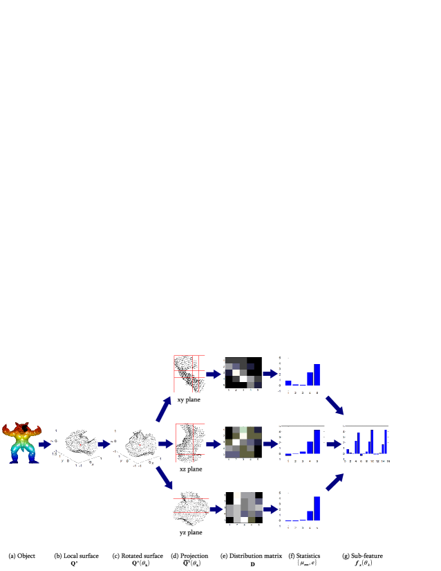
First, the pointcloud is rotated around the $x$ axis by an angle $\theta_{k}$, resulting in a rotated pointcloud $\mathbf{Q}^{\prime}\left(\theta_{k}\right)$, as shown in Fig. 4(c). This pointcloud $\mathbf{Q}^{\prime}\left(\theta_{k}\right)$ is then projected onto three coordinate planes (i.e., the $xy$, $xz$ and $yz$ planes) to obtain three projected pointclouds $\widetilde{\mathbf{Q}^{\prime}}_{i}\left(\theta_{k}\right),i=1,2,3$. Note that, the projection offers a means to describe the 3D local surface in a concise and efficient manner. That is because 2D projections clearly preserve a certain amount of unique 3D geometric information of the local surface from that particular viewpoint.

Next, for each projected pointcloud $\widetilde{\mathbf{Q}^{\prime}}_{i}\left(\theta_{k}\right)$, a 2D bounding rectangle is obtained, which is subsequently divided into $L\times L$ bins, as shown in Fig. 4(d). The number of points falling into each bin is then counted to yield an $L\times L$ matrix $\mathbf{D}$, as shown in Fig. 4(e). We refer to the matrix $\mathbf{D}$ as a “distribution matrix” since it represents the 2D distribution of the neighboring points. The distribution matrix $\mathbf{D}$ is further normalized such that the sum of all bins is equal to one in order to achieve invariance to variations in mesh resolution.

The information in the distribution matrix $\mathbf{D}$ is further condensed in order to achieve computational and storage efficiency. In this paper, a set of statistics is extracted from the distribution matrix $\mathbf{D}$, including central moments (Demi et al., 2000; Hu, 1962) and Shannon entropy (Shannon, 1948). The central moments are utilized for their mathematical simplicity and rich descriptiveness (Hu, 1962), while Shannon entropy is selected for its strong power to measure the information contained in a probability distribution (Shannon, 1948).

The central moment $\mu_{mn}$ of order $m+n$ of matrix $\mathbf{D}$ is defined as:

$$\mu_{mn}=\sum_{i=1}^{L}\sum_{j=1}^{L}\left(i-\bar{i}\right)^{m}\left(j-\bar{j}\right)^{n}\mathbf{D}\left(i,j\right),$$ (12)

where

$$\bar{i}=\sum_{i=1}^{L}\sum_{j=1}^{L}i\mathbf{D}\left(i,j\right),$$ (13)

and

$$\bar{j}=\sum_{i=1}^{L}\sum_{j=1}^{L}j\mathbf{D}\left(i,j\right).$$ (14)

The Shannon entropy $e$ is calculated as:

$$e=-\sum_{i=1}^{L}\sum_{j=1}^{L}\mathbf{D}\left(i,j\right)\log\left(\mathbf{D}\left(i,j\right)\right).$$ (15)

Theoretically, a complete set of central moments can be used to uniquely describe the information contained in a matrix (Hu, 1962). However in practice, only a small subset of the central moments can sufficiently represent the distribution matrix $\mathbf{D}$. These selected central moments together with the Shannon entropy are then used to form a statistics vector, as shown in Fig. 4(f). The three statistics vectors from the $xy$, $xz$ and $yz$ planes are then concatenated to form a sub-feature $\boldsymbol{f}_{x}\left(\theta_{k}\right)$. Note that $\boldsymbol{f}_{x}\left(\theta_{k}\right)$ denotes the total statistics for the $k$th rotation around the $x$ axis, as shown in Fig. 4(g).

In order to encode the “complete” information of the local surface, the pointcloud $\mathbf{Q}^{\prime}$ is rotated around the $x$ axis by a set of angles $\left\{\theta_{k}\right\},k=1,2,\ldots,T$, resulting in a set of sub-features $\left\{\boldsymbol{f}_{x}\left(\theta_{k}\right)\right\},k=1,2,\ldots,T$. Further, $\mathbf{Q}^{\prime}$ is rotated by a set of angles around the $y$ axis and a set of sub-features $\left\{\boldsymbol{f}_{y}\left(\theta_{k}\right)\right\},k=1,2,\ldots,T$ is calculated. Finally, $\mathbf{Q}^{\prime}$ is rotated by a set of angles around the $z$ axis and a set of sub-features $\left\{\boldsymbol{f}_{z}\left(\theta_{k}\right)\right\},k=1,2,\ldots,T$ is calculated. The overall feature descriptor is then generated by concatenating the sub-features of all the rotations into a vector, that is:

$$\boldsymbol{f}=\left\{\boldsymbol{f}_{x}\left(\theta_{k}\right),\boldsymbol{f}_{y}\left(\theta_{k}\right),\boldsymbol{f}_{z}\left(\theta_{k}\right)\right\},k=1,2,\ldots,T.$$ (16)

It is expected that the RoPS descriptor would be highly discriminative (as demonstrated in Section 5) since it encodes the geometric information of a local surface from a set of viewpoints. Note that, some existing view-based methods can be found in the literature, such as (Yamauchi et al., 2006), (Ohbuchi et al., 2008) and (Atmosukarto and Shapiro, 2010). However, these methods are based on global features and originate from the 3D shape retrieval area. They are, however, not suitable for 3D object recognition due to their sensitivity to occlusion and clutter.

Other related methods, however, include the spin image (Johnson and Hebert, 1999) and snapshot (Malassiotis and Strintzis, 2007) descriptors. A spin image is generated by projecting a local surface onto a 2D plane using a cylindrical parametrization. Similarly, a snapshot is obtained by rendering a local surface from the viewpoint which is perpendicular to the surface. Our RoPS differs from these methods in several aspects. First, RoPS represents a local surface from a set of viewpoints rather than just one view (as in the case of spin image and snapshot). Second, RoPS is associated with a unique and unambiguous LRF, and it is invariant to rotation. In contrast, spin image discards cylindrical angular information and snapshot is prone to rotation. Third, RoPS is more compact than spin image and snapshot since RoPS further encodes 2D matrices with a set of statistics. The typical lengths of RoPS, spin image and snapshot are 135, 225 and 1600, respectively (see Table 2, (Johnson and Hebert, 1999) and (Malassiotis and Strintzis, 2007)).

4.2 RoPS Generation Parameters

The RoPS feature descriptor has four parameters: i) the combination of statistics, ii) the number of partition bins $L$, iii) the number of rotations $T$ around each coordinate axis, and iv) the support radius $r$. The performance of RoPS descriptor against different settings of these parameters was tested on the Tuning Dataset using the criterion of Recall vs 1-Precision Curve (RP Curve).

RP Curve is one of the most popular criteria used for the assessment of a feature descriptor (Flint et al., 2008; Hou and Qin, 2010; Ke and Sukthankar, 2004; Mikolajczyk and Schmid, 2005). It is calculated as follows: given a scene, a model and the ground truth transformation, a scene feature is matched against all model features to find the closest feature. If the ratio between the smallest distance and the second smallest one is less than a threshold, then the scene feature and the closest model feature are considered a match. Further, a match is considered a true positive only if the distance between the physical locations of the two features is sufficiently small, otherwise it is considered a false positive. Therefore, recall is defined as:

$$\textrm{recall}=\frac{\textrm{the number of true positives}}{\textrm{total number of positives}}.$$ (17)

1-precision is defined as:

$$\textrm{1-precision}=\frac{\textrm{the number of false positives}}{\textrm{total number of matches}}.$$ (18)

By varying the threshold, a RP Curve can be generated. Ideally, a RP Curve would fall in the top left corner of the plot, which means that the feature obtains both high recall and precision.

(a)

(b)

(c)

(d)

Figure 5: Effect of the RoPS generation parameters. (a) Different combinations of statistics. (b) The number of partition bins $L$. There is a twin plot in (b), where the right plot is a magnified version of the region indicated by the rectangle in the left plot. (c) The number of rotations $T$. There is a twin plot in (c), where the right plot is a magnified version of the region indicated by the rectangle in the left plot. (d) The support radius $r$. (We chose the No.6 combination of the statistics and set $L=5$, $T=3$ and $r=15$mr in this paper as a tradeoff between effectiveness and efficiency. Figure best seen in color.)

4.2.1 The Combination of Statistics

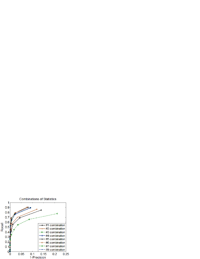
The selection of the subset of statistics plays an important role in the generation of a RoPS feature descriptor. It determines not only the capability for encapsulating the information in a distribution matrix but also the size of a feature vector. We considered eight combinations of statistics (a number of low-order moments and entropy), as listed in Table 1, and tested the performance for each combination in the terms of RP Curve. The other three parameters were set constant as $L=5$, $T=3$ and $r=15$mr. It is worth noting that the zeroth-order central moment $\mu_{00}$ and the first-order central moments $\mu_{01}$ and $\mu_{10}$ were excluded from the combinations of the statistics. Because these moments are constant (i.e., $\mu_{00}=1$, $\mu_{01}=0$ and $\mu_{10}=0$) and therefore contain no information of the local surface. Our experimental results are shown in Fig. 5(a).

Table 1: Different combinations of the statistics.

No.	Combination of the statistics
1	$\mu_{02},\mu_{11},\mu_{20}$
2	$\mu_{02},\mu_{11},\mu_{20}$,$\mu_{03},\mu_{12},\mu_{21},\mu_{30}$
3	$\mu_{02},\mu_{11},\mu_{20}$,$\mu_{03},\mu_{12},\mu_{21},\mu_{30}$,$\mu_{04},\mu_{13},\mu_{22},\mu_{31},\mu_{40}$
4	$\mu_{02},\mu_{11},\mu_{20}$,$\mu_{03},\mu_{12},\mu_{21},\mu_{30}$,$\mu_{04},\mu_{13},\mu_{22},\mu_{31},\mu_{40},e$
5	$\mu_{11},\mu_{21},\mu_{12},\mu_{22}$
6	$\mu_{11},\mu_{21},\mu_{12},\mu_{22},e$
7	$\mu_{11},\mu_{21},\mu_{12},\mu_{22},\mu_{31},\mu_{13}$
8	$\mu_{11},\mu_{21},\mu_{12},\mu_{22},\mu_{31},\mu_{13},e$

It is clear that the No.6 combination achieved the best performance, followed by the No.5 combination. While the No.3, No.4 and No.8 combinations obtained comparable performance, with recall being a little lower than the No.6 combination. The superior performance of the No.6 combination is due to the facts that, first, the low-order moments $\mu_{11},\mu_{21},\mu_{12},\mu_{22}$ and entropy $e$ contain the most meaningful and significant information of the distribution matrix. Consequently, the descriptiveness of these statistics is sufficiently high. Second, the low-order moments are more robust to noise and varying mesh resolution compared to the high-order moments. Beyond the high precision and recall, the size of the No.6 combination is also small, which means that the calculation and matching of feature descriptors can be performed efficiently. Therefore, the No.6 combination, i.e., $\left\{\mu_{11},\mu_{21},\mu_{12},\mu_{22},e\right\}$, was selected to represent the information in a distribution matrix and to form the RoPS descriptor.

4.2.2 The Number of Partition Bins

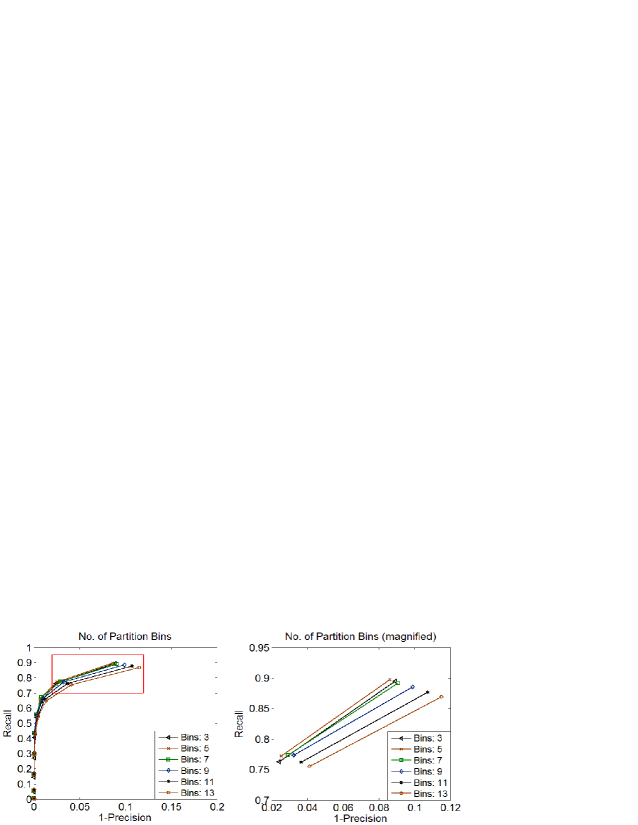
The number of partition bins $L$ is another important parameter in the RoPS generation. It determines both the descriptiveness and robustness of a descriptor. That is, a dense partition of the projected points offers more details about the point distribution, it however increases the sensitivity to noise and varying mesh resolution. We tested the performance of RoPS descriptor on the Tuning Dataset with respect to a number of partition bin, while the two other parameters were set to $T=3$ and $r=15$mr. The experimental results are shown in Fig. 5(b) as a twin plot, where the right plot is a magnified version of the region indicated by the rectangle in the left plot.

The plot shows that the performance of RoPS descriptor improved as the number of partition bins increased from 3 to 5. This is because more details about the point distribution were encoded into the feature descriptor. However, for a number of partition bins larger than 5, the performance degraded as the number of partition bins increased. This is due to the reason that a dense partition makes the distribution matrix more susceptible to the variation of spatial position of the neighboring points. It can therefore be inferred that 5 is the most suitable number of partitions as a tradeoff between the descriptiveness and the robustness to noise and varying mesh resolution. We therefore used $L=5$ in this paper.

4.2.3 The Numbers of Rotations

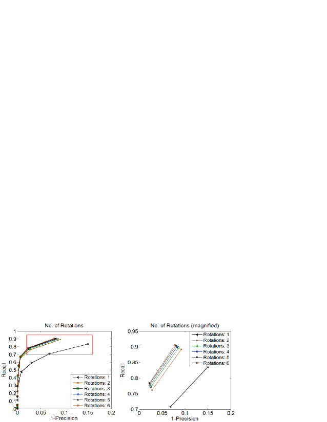
The number of rotations $T$ determines the “completeness” when describing the local surface using a RoPS feature descriptor. That is, increasing the number of rotations means that more information of the local surface are encoded into the overall feature descriptor. We tested the performance of the RoPS feature descriptor with respect to a varying number of rotations while keeping the other parameters constant (i.e., $r=15$mr). The results are given in Fig. 5(c) as a twin plot, where the right plot is a magnified version of the region indicated by the rectangle in the left plot.

It was found that as the number of rotations increased, the descriptiveness of the RoPS increased, resulting in an improvement of the matching performance (which confirmed our assumption). Specifically, the performance of the RoPS descriptor improved significantly as the number of rotations increased from 1 to 2, as shown in the left plot of Fig. 5(c). The performance then improved slightly as the number of rotations increased from 2 to 6, as indicated in the magnified version shown in the right plot of Fig. 5(c). In fact, there was no notable difference between the performance with respect to the number of rotations of 3 and 6. That is because almost all the information of the local surface is encoded in the feature descriptor by rotating the neighboring points 3 times around each axis. Therefore, increasing the number of rotations any further will not necessarily add any significant information to the feature descriptor. Moreover, increasing the number of rotations will cost more computational and memory resources. We therefore, set the number of rotations to be 3 in this paper.

4.2.4 The Support Radius

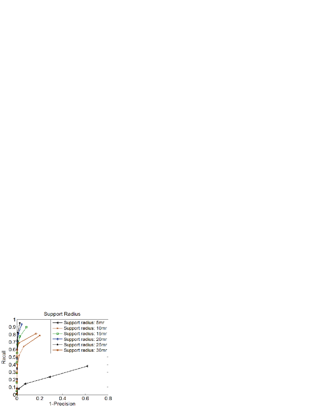
The support radius $r$ determines the amount of surface that is encoded by the RoPS feature descriptor. The value of $r$ can be chosen depending on how local the feature should be, and a tradeoff lies between the feature’s descriptiveness and robustness to occlusion. That is, a large support radius enables the RoPS descriptor to encapsulate more information of the object and therefore provides more descriptiveness. On the other hand, a large support radius increases the sensitivity to occlusion and clutter. We tested the performance of the RoPS feature descriptor with respect to varying support radius while keeping the other parameters fixed. The results are given in Fig. 5(d).

The results show that the recall and precision performance of the RoPS feature descriptor improved steadily as the support radius increased from 5mr (mr = mesh resolution) to 25mr. Specifically, there was a significant improvement of the matching performance as the support radius increased from 5mr to 10mr, this is because a radius of 5mr is too small to contain sufficient discriminating information of the underlying surface. The RoPS feature descriptor achieved good results with a support radius of 15mr, achieving a high precision of about 0.9 and a high recall of about 0.9. Although the performance of RoPS feature descriptor further improved slightly as the support radius was increased to 25mr, the performance deteriorated sharply when the support radius was set to 30mr. We choose to set the support radius to 15mr in the paper to maintain a strong robustness to occlusion and clutter. An illustration is shown in Fig. 6. The range image contains two objects in the presence of occlusion and clutter, and a feature point is selected near the tail of the chicken. The red, green and blue spheres, respectively represent the support regions with radius of 25 mr, 15mr and 5mr for the feature point. As the radius increases from 5mr to 25 mr, points on the surface within the support region are more likely to be missing due to occlusion, and points from other objects (e.g., T-rex on the right) are more likely to be included in the support region due to clutter. Therefore, the resulting feature descriptor is more likely to be affected by occlusion and clutter.

Figure 6: An illustration of the descriptor’s robustness to occlusion and clutter with respect to varying support radius. The red, green and blue spheres respectively represent the support regions with radius of 25 mr, 15mr and 5mr for a feature point. (Figure best seen in color.)

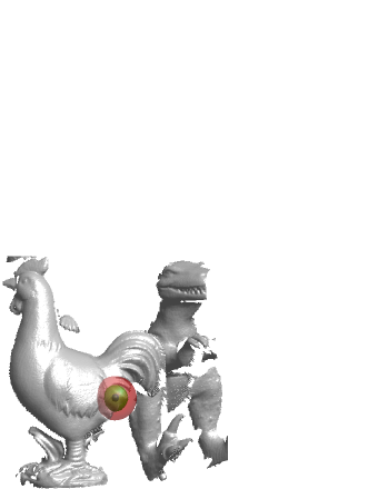
Note that, several adaptive-scale keypoint detection methods have been proposed for the purpose of determining the support radius based on the inherent scale of a feature point (Tombari et al., 2013). However, we simply adopt a fixed support radius since our focus is on feature description and object recognition rather than keypoint detection. Moreover, our proposed RoPS descriptor has been demonstrated to achieve an even better performance compared to the methods with adaptive-scale keypoint detection (e.g., EM matching and keypoint matching), as analyzed in Section 7.

5 Performance of the RoPS Descriptor

The descriptiveness and robustness of our proposed RoPS feature descriptor was first evaluated on the Bologna Dataset (Tombari et al., 2010) with respect to different levels of noise, varying mesh resolution and their combinations. It was also evaluated on the PHOTOMESH Dataset (Zaharescu et al., 2012) with respect to 13 transformations. In these experiments, the RoPS was compared to several state-of-the-art feature descriptors.

5.1 Performance on The Bologna Dataset

5.1.1 Dataset and Parameter Setting

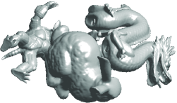
The Bologna Dataset used in this paper comprises six models and 45 scenes. The six models (i.e., “Armadillo”, “Asia Dragon”, “Bunny”, “Dragon”, “Happy Buddha” and “Thai Statue”) were taken from the Stanford 3D Scanning Repository. They are shown in Fig. 2. Each scene was synthetically generated by randomly rotating and translating three to five models in order to create clutter and pose variances. As a result, the ground truth rotations and translations between each model and its instances in the scenes were known a priori during the process of construction. An example scene is shown in Fig. 7.

Figure 7: A scene on the Bologna Dataset.

The performance of each feature descriptor was assessed using the criterion of RP Curve (as detailed in Section 4.2). We compared our RoPS feature descriptor with five state-of-the-art feature descriptors, including spin image (Johnson and Hebert, 1999), normal histogram (NormHist) (Hetzel et al., 2001), LSP (Chen and Bhanu, 2007), THRIFT (Flint et al., 2007) and SHOT (Tombari et al., 2010). The support radius $r$ for all methods was set to be 15mr as a compromise between the descriptiveness and the robustness to occlusion. The parameters for generating all these feature descriptors were tuned by optimizing the performance in terms of RP Curve on the Tuning Dataset. The tuned parameter settings for all feature descriptors are presented in Table 2.

Table 2: Tuned parameter settings for six feature descriptors.

	Support Radius	Dimensionality	Length
Spin image	15mr	15*15	225
NormHist	15mr	15*15	225
LSP	15mr	15*15	225
THRIFT	15mr	32*1	32
SHOT	15mr	8*2*2*10	320
RoPS	15mr	3*3*3*5	135

In order to avoid the impact of the keypoint detection method on feature’s descriptiveness, we randomly selected 1000 feature points from each model, and extracted their corresponding points from the scene. We then employed the methods listed in Table 2 to extract feature descriptors for these feature points. Finally, we calculated a RP Curve for each feature descriptor to evaluate the performance.

5.1.2 Robustness to Noise

(a) Noise free

(b) Noise with a standard deviation of 0.1mr

(c) Noise with a standard deviation of 0.2mr

(d) Noise with a standard deviation of 0.3mr

(e) Noise with a standard deviation of 0.4mr

(f) Noise with a standard deviation of 0.5mr

Figure 8: Recall vs 1-Precision curves in the presence of noise. (Figure best seen in color.)

(a) $\nicefrac{{1}}{{2}}$ mesh decimation

(b) $\nicefrac{{1}}{{4}}$ mesh decimation

(c) $\nicefrac{{1}}{{8}}$ mesh decimation

(d) $\nicefrac{{1}}{{2}}$ mesh decimation and 0.1mr Gaussian noise

Figure 9: Recall vs 1-Precision curves with respect to mesh resolution. (Figure best seen in color.)

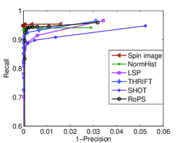
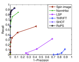
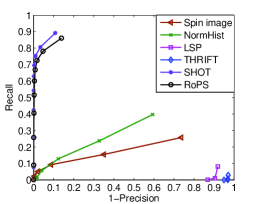
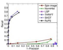
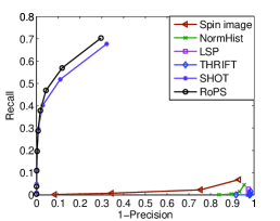
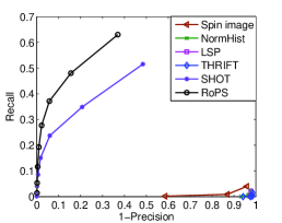
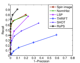
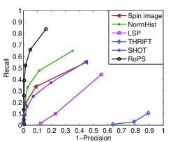
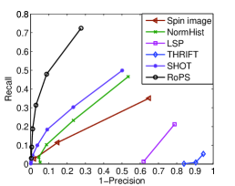
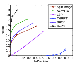
In order to evaluate the robustness of these feature descriptors to noise, we added a Gaussian noise with increasing standard deviation of 0.1mr, 0.2mr, 0.3mr, 0.4mr and 0.5mr to the scene data. The RP Curves under different levels of noise are presented in Fig. 8.

We made a number of observations. i) These feature descriptors achieved comparable performance on noise free data, with high recall together with high precision, as shown in Fig. 8(a).

ii) With noise, our proposed RoPS feature descriptor achieved the best performance in most cases, and is followed by SHOT. Specifically, the performance of RoPS is better than SHOT under a low-level noise with a standard deviation of 0.1mr, as shown in Fig. 8(b). As the standard deviation of the noise increased to 0.2mr and 0.3mr, SHOT performed slightly better than RoPS, as indicated in Figures 8(c) and (d). However, the performance of our proposed RoPS was significantly better than SHOT under high levels of noise, e.g., with a noise deviation larger than 0.3mr, as shown in Figures 8(e) and (f). It can be inferred that RoPS is very robust to noise, particularly in the case of scenes with a high level of noise.

iii) As the noise level increased, the performance of LSP and THRIFT deteriorated sharply, as shown in Figures 8(b-e). THRIFT failed to work even under a low-level of noise with a standard deviation of 0.1mr. This result is also consistent with the conclusion given in (Flint et al., 2008). Although NormHist and spin image worked relatively well under low- and medium-level noise with a standard deviation less than 0.2mr, they failed completely under noise with a large standard deviation. The sensitivity of spin image, NormHist, THR-IFT and LSP to noise is due to the fact that, they rely on surface normals to generate their feature descriptors. Since the calculation of surface normal includes a process of differentiation, it is very susceptible to noise.

iv) The strong robustness of our RoPS feature descriptor to noise can be explained by at least three facts. First, RoPS encodes the “complete” information of the local surface from various viewpoints through rotation and therefore, encodes more information than the existing methods. Second, RoPS only uses the low-order moments of the distribution matrices to form its feature descriptor and is therefore less affected by noise. Third, our proposed unique, unambiguous and stable LRF also helps to increase the descriptiveness and robustness of the RoPS feature descriptor.

5.1.3 Robustness to Varying Mesh Resolution

In order to evaluate the robustness of these feature descriptors to varying mesh resolution, we resampled the noise free scene meshes to $\nicefrac{{1}}{{2}}$, $\nicefrac{{1}}{{4}}$ and $\nicefrac{{1}}{{8}}$ of their original mesh resolution. The RP Curves under different levels of mesh decimation are presented in Figures 9(a-c).

It was found that our proposed RoPS feature descriptor outperformed all the other descriptors by a large margin under all levels of mesh decimation. It is also notable that the performance of our RoPS feature descriptor with $\nicefrac{{1}}{{8}}$ of original mesh resolution was even comparable to the best results given by the existing feature descriptors with $\nicefrac{{1}}{{2}}$ of original mesh resolution. Specifically, RoPS obtained a precision more than 0.7 and a recall more than 0.7 with $\nicefrac{{1}}{{8}}$ of original mesh resolution, whereas spin image obtained a precision around 0.8 and a recall around 0.8 with $\nicefrac{{1}}{{2}}$ of original mesh resolution, as shown in Figures 9(a) and (c). This indicated that our RoPS feature descriptor is very robust to varying mesh resolution.

The strong robustness of RoPS to varying mesh resolution is due to at least two factors. First, the LRF of RoPS is derived by calculating the scatter matrix of all the points lying on the local surface rather than just the vertices, which makes RoPS robust to different mesh resolution. Second, the 2D projection planes are sparsely partitioned and only the low-order moments are used to form the feature descriptor, which further improves the robustness of our method to mesh resolution.

5.1.4 Robustness to Combined Noise and Mesh Decimation

In order to further test the robustness of these feature descriptors to combined noise and mesh decimation, we resampled the scene meshes down to $\nicefrac{{1}}{{2}}$ of their original mesh resolution and added a Gaussian random noise with a standard deviation of 0.1mr to the scenes. The resulting RP Curves are presented in Fig. 9(d).

As shown in Fig. 9(d), RoPS significantly outperformed the other methods in the scenes with both noise and mesh decimation, obtaining a high precision of about 0.9 and a high recall of about 0.9. It is followed by NormHist, SHOT, spin image and LSP, while THRIFT failed to work.

As summarized in Table 2, the RoPS feature descriptor length is 135, while the others such as spin image, NormHist, LSP and SHOT are 225, 225, 225 and 320, respectively. So RoPS is more compact and therefore more efficient for feature matching compared to these methods. Note that, although the length of THRIFT is smaller than RoPS, THRIFT’s performance in terms of recall and precision results is surpassed by our RoPS feature descriptor by a large margin.

5.2 Performance on The PHOTOMESH Dataset

The PHOTOMESH Dataset contains three null shapes. Two of the null shapes were obtained with multi-view stereo reconstruction algorithms, and the other one was generated with a modeling program. 13 transformations were applied to each shape. The transformations include color noise, color shot noise, geometry noise, geometry shot noise, rotation, scale, local scale, sampling, hole, micro-hole, topology changes and isometry. Each transformation has five different levels of strength.

To make a rigorous comparison with (Zaharescu et al., 2012), we set the support radius $r$ to $\sqrt{\nicefrac{{\alpha_{r}A_{M}}}{{\pi}}}$, where $A_{M}$ is the total area of a mesh, and $\alpha_{r}$ is 2%. RoPS feature descriptors were calculated at all points of the shapes, without any feature detection. We used the average normalized $L_{2}$ distance between the feature descriptors of corresponding points to measure the quality of a feature descriptor, as in (Zaharescu et al., 2012). The experimental results of the RoPS descriptor are shown in Table 3. For comparison, the results of the MeshHOG descriptor (Gaussian curvature) without and with MeshDOG are also reported in Tables 4 and 5, respectively.

The RoPS descriptor was clearly invariant to color noise and color shot noise. Because the geometric information used in RoPS cannot be affected by color deformations. RoPS was also invariant to rotation and scale, which means that it was invariant to rigid transformations.

The RoPS descriptor turned out to be very robust to geometry noise, geometry shot noise, local scale, holes, micro-holes, topology and isometry with noise. The average normalized $L_{2}$ distances for all these transformations were no more than 0.06, even under the highest level of transformations. The biggest challenge for RoPS descriptor was sampling. The average normalized $L_{2}$ distance increased from 0.01 to 0.06 as the strength level changed from 1 to 5. However, RoPS was more robust to sampling than MeshHOG. As shown in Tables 3 and 4, the average normalized $L_{2}$ distance of RoPS with a strength level of 5 was even smaller than that of MeshHOG with a strength level of 1, i.e., 0.02 and 0.04, respectively. Overall, the average normalized $L_{2}$ distances of RoPS descriptor were much smaller under all strength levels of all transformations compared to MeshHOG.

Table 3: Robustness of RoPS descriptor.

	Strength
Transform.	1	$\leq$2	$\leq$3	$\leq$4	$\leq$5
Color Noise	0.00	0.00	0.00	0.00	0.00
Color Shot Noise	0.00	0.00	0.00	0.00	0.00
Geometry Noise	0.01	0.01	0.01	0.02	0.02
Geometry Shot Noise	0.01	0.01	0.02	0.03	0.05
Rotation	0.00	0.00	0.00	0.00	0.00
Scale	0.00	0.00	0.00	0.00	0.00
Local Scale	0.01	0.01	0.02	0.02	0.02
Sampling	0.01	0.02	0.04	0.05	0.06
Holes	0.01	0.01	0.01	0.01	0.02
Marco-Holes	0.00	0.01	0.01	0.01	0.01
Topology	0.01	0.01	0.02	0.02	0.03
Isometry + Noise	0.02	0.02	0.01	0.02	0.02
Average	0.00	0.01	0.01	0.02	0.02

Table 4: Robustness of MeshHOG (Gaussian curvature) without MeshDOG detector.

	Strength
Transform.	1	$\leq$2	$\leq$3	$\leq$4	$\leq$5
Color Noise	0.00	0.00	0.00	0.00	0.00
Color Shot Noise	0.00	0.00	0.00	0.00	0.00
Geometry Noise	0.07	0.08	0.09	0.10	0.11
Geometry Shot Noise	0.02	0.03	0.05	0.06	0.09
Rotation	0.00	0.00	0.00	0.00	0.00
Scale	0.00	0.00	0.00	0.00	0.00
Local Scale	0.06	0.07	0.08	0.09	0.10
Sampling	0.10	0.12	0.13	0.13	0.13
Holes	0.01	0.02	0.04	0.03	0.05
Marco-Holes	0.01	0.01	0.03	0.04	0.04
Topology	0.07	0.10	0.11	0.11	0.12
Isometry + Noise	0.08	0.08	0.08	0.09	0.09
Average	0.04	0.04	0.05	0.06	0.06

6 3D Object Recognition Algorithm

So far we have developed a novel LRF and a RoPS feature descriptor. In this section, we propose a new hierarchical 3D object recognition algorithm based on the LRF and RoPS descriptor. Our 3D object recognition algorithm consists of four major modules, i.e., model representation, candidate model generation, transformation hypothesis generation, verification and segmentation. A flow chart illustration of the algorithm is given in Fig. 10.

Table 5: Robustness of MeshHOG (Gaussian curvature) with MeshDOG detector.

	Strength
Transform.	1	$\leq$2	$\leq$3	$\leq$4	$\leq$5
Color Noise	0.00	0.00	0.00	0.00	0.00
Color Shot Noise	0.00	0.00	0.00	0.00	0.00
Geometry Noise	0.26	0.29	0.31	0.33	0.34
Geometry Shot Noise	0.04	0.09	0.14	0.21	0.29
Rotation	0.01	0.01	0.01	0.01	0.01
Scale	0.01	0.01	0.01	0.01	0.00
Local Scale	0.21	0.25	0.28	0.30	0.31
Sampling	0.31	0.34	0.34	0.36	0.36
Holes	0.02	0.02	0.07	0.07	0.07
Marco-Holes	0.01	0.01	0.07	0.07	0.08
Topology	0.13	0.20	0.22	0.25	0.28
Isometry + Noise	0.23	0.24	0.22	0.25	0.25
Average	0.10	0.12	0.14	0.15	0.17

Figure 10: Flow chart of the 3D object recognition algorithm. The module of model representation is performed offline, and the other modules are operated online.

6.1 Model Representation

We first construct a model library for the 3D objects that we are interested in. Given a model $\mathsf{\mathscr{\mathcal{M}}}$, $N_{m}$ seed points are evenly selected from the model pointcloud. Since the feature descriptors of closely located feature points may be similar (since they represent more or less the same local surface), a resolution control strategy (Zhong, 2009) is further enforced on these seed points to extract the final feature points. For each feature point $\boldsymbol{p}_{m}$, the LRF $\mathbf{F}_{m}$ and the feature descriptor (e.g., our RoPS descriptor) $\boldsymbol{f}_{m}$ are calculated. The point position $\boldsymbol{p}_{m}$, LRF $\mathbf{F}_{m}$ and feature descriptor $\boldsymbol{f}_{m}$ of all the feature points are then stored in a library for object recognition.

In order to speed up the process of feature matching during online recognition, the local feature descriptors from all models are indexed using a $k$-d tree method (Bentley, 1975). Note that, the model feature calculation and indexing can be performed offline, while the following modules are operated online.

6.2 Candidate Model Generation

The input scene $\mathcal{S}$ is first decimated, which results in a low resolution mesh $\mathcal{S}^{\prime}$. The vertices of $\mathcal{S}$ which are nearest to the vertices of $\mathcal{S}^{\prime}$ are selected as seed points (following a similar approach of (Mian et al., 2006b)). Next, a resolution control strategy (Zhong, 2009) is enforced on these seed points to prune out redundant seed points. A boundary checking strategy (Mian et al., 2010) is also applied to the seed points to eliminate the boundary points of the range image. Further, since the LRF of a point can be ambiguous when two eigenvalues of the overall scatter matrix of the underlying local surface (see Eq. 4) are equal, we impose a constraint on the ratios of the eigenvalues $\nicefrac{{\lambda_{1}}}{{\lambda_{2}}}>\tau_{\lambda}$ to exclude seed points with symmetrical local surfaces, as in (Zhong, 2009; Mian et al., 2010). The remaining seed points are considered feature points. It is worth noting that, the feature point detection and LRF calculation procedures can be performed simultaneously. Given the LRF $\mathbf{F}_{s}$ of a feature point $\boldsymbol{p}_{s}$, its feature descriptor $\boldsymbol{f}_{s}$ is subsequently calculated.

The scene features are exactly matched against all model features in the library using the previously constructed $k$-d tree. If the ratio between the smallest distance and the second smallest one is less than a threshold $\tau_{f}$, the scene feature and its closest model feature are considered a feature correspondence. Each feature correspondence votes for a model. These models which have received votes from feature correspondences are considered candidate models. They are then ranked according to the number of votes received. With this ranked models, the subsequent steps (Sections 6.3 and 6.4) can be performed from the most likely candidate model.

6.3 Transformation hypothesis Generation

For a feature correspondence which votes for the model $\mathsf{\mathscr{\mathcal{M}}}$, a rigid transformation is calculated by aligning the LRF of the model feature to the LRF of the scene feature. Specifically, given the LRF $\mathbf{F}_{s}$ and the point position $\boldsymbol{p}_{s}$ of a scene feature, the LRF $\mathbf{F}_{m}$ and the point position $\boldsymbol{p}_{m}$ of a corresponding model feature, the rigid transformation can be estimated by:

$$\mathbf{R}=\mathbf{F}_{s}^{\mathrm{T}}\mathbf{F}_{m},$$ (19)

$$\boldsymbol{t}=\boldsymbol{p}_{s}-\boldsymbol{p}_{m}\mathbf{R},$$ (20)

where $\mathbf{R}$ is the rotation matrix and $\boldsymbol{t}$ is the translation vector of the rigid transformation. It is worth noting that a transformation can be estimated from a single feature correspondence using our RoPS feature descriptor. This is a major advantage of our algorithm compared with most of the existing algorithms (e.g., splash, point signatures and spin image based methods) which require at least three correspondences to calculate a transformation (Johnson and Hebert, 1999). Our algorithm not only eliminates the combinatorial explosion of feature correspondences but also improves the reliability of the estimated transformation.

As all the plausible transformations $\left(\mathbf{R}_{i},\boldsymbol{t}_{i}\right),i=1,2,\cdots,N_{t}$ between the scene $\mathcal{S}$ and the model $\mathsf{\mathscr{\mathcal{M}}}$ are calculated, these transformations are then grouped into several clusters. Specifically, for each plausible transformation, its rotation matrix $\mathbf{R}_{i}$ is first converted into three Euler angles which form a vector $\boldsymbol{u}_{i}$. In this manner, the difference between any two rotation matrices can be measured by the Euclidean distance between their corresponding Euler angles. These transformations whose Euler angles are around $\boldsymbol{u}_{i}$ (with distances less than $\tau_{a}$) and translations are around $\boldsymbol{t}_{i}$ (with distances less than $\tau_{t}$) are grouped into a cluster $\mathcal{C}_{i}$. Therefore, each plausible transformation $\left(\mathbf{R}_{i},\boldsymbol{t}_{i}\right)$ results in a cluster $\mathcal{C}_{i}$. The cluster center $\left(\mathbf{R}_{c},\boldsymbol{t}_{c}\right)$ of $\mathcal{C}_{i}$ is calculated as the average rotation and translation in that cluster. Next, a confidence score $s_{c}$ for each cluster is calculated as:

$$s_{c}=\frac{n_{f}}{d},$$ (21)

where $n_{f}$ is the number of feature correspondences in the cluster, and $d$ is the average distance between the scene features and their corresponding model features which fall within the cluster. These clusters are sorted according to their confidence scores, the ones with confidence scores smaller than half of the maximum score are first pruned out. We then select the valid clusters from these remaining clusters, starting from the highest scored one and discarding the nearby clusters whose distances to these selected clusters are small (using $\tau_{a}$ and $\tau_{t}$). $\tau_{a}$ and $\tau_{t}$ are empirically set to 0.2 and 30mr throughout this paper. These selected clusters are then allowed to proceed to the final verification and segmentation stage (Section 6.4).

6.4 Verification and Segmentation

Given a scene $\mathcal{S}$, a candidate model $\mathsf{\mathscr{\mathcal{M}}}$ and a transformation hypothesis $\left(\mathbf{R}_{c},\boldsymbol{t}_{c}\right)$, the model $\mathsf{\mathscr{\mathcal{M}}}$ is first transformed to the scene $\mathcal{S}$ by using the transformation hypothesis $\left(\mathbf{R}_{c},\boldsymbol{t}_{c}\right)$. This transformation is further refined using the ICP algorithm (Besl and McKay, 1992), resulting in a residual error $\varepsilon$. After ICP refinement, the visible proportion $\alpha$ is calculated as:

$$\alpha=\frac{n_{c}}{n_{s}},$$ (22)

where $n_{c}$ is the number of corresponding points between the scene $\mathcal{S}$ and the model $\mathsf{\mathscr{\mathcal{M}}}$, $n_{s}$ is the total number of points in the scene $\mathcal{S}$. Here, a scene point and a transformed model point are considered corresponding if their distance is less than twice the model resolution (Mian et al., 2006b).

The candidate model $\mathsf{\mathscr{\mathcal{M}}}$ and the transformation hypothesis $\left(\mathbf{R}_{c},\boldsymbol{t}_{c}\right)$ are accepted as being correct only if the residual error $\varepsilon$ is smaller than a threshold $\tau_{\varepsilon}$ and the proportion $\alpha$ is larger than a threshold $\tau_{\alpha}$. However, it is hard to determine the thresholds. Because selecting strict thresholds will reject correct hypotheses which are highly occluded in the scene, while selecting loose thresholds will produce many false positives. In this paper, a flexible thresholding scheme is developed. To deal with a highly occluded but well aligned object, we select a small error threshold $\tau_{\varepsilon 1}$ together with a small proportion threshold $\tau_{\alpha 1}$. Meanwhile, in order to increase the tolerance to the residual error which resulted from an inaccurate estimation of the transformation, we select a relatively larger error threshold $\tau_{\varepsilon 2}$ together with a larger proportion threshold $\tau_{\alpha 2}$. We chose these thresholds empirically and set them as $\tau_{\varepsilon 1}=0.75\textrm{mr}$, $\tau_{\varepsilon 2}=1.5\textrm{mr}$, $\tau_{\alpha 1}=0.04$ and $\tau_{\alpha 2}=0.2$ throughout the paper.

Therefore, once $\varepsilon<\tau_{\varepsilon 1}$ but $\alpha>\tau_{\alpha 1}$, or $\varepsilon<\tau_{\varepsilon 2}$ but $\alpha>\tau_{\alpha 2}$, the candidate model $\mathsf{\mathscr{\mathcal{M}}}$ and the transformation hypothesis $\left(\mathbf{R}_{c},\boldsymbol{t}_{c}\right)$ are accepted, the scene points which correspond to this model are removed from the scene. Otherwise, this transformation hypothesis is rejected and the next transformation hypothesis is verified by turn. If no transformation hypothesis results in an accurate alignment, we conclude that the model $\mathsf{\mathscr{\mathcal{M}}}$ is not present in the scene $\mathcal{S}$. While if more than one transformation hypotheses are accepted, it means that multiple instances of the model $\mathsf{\mathscr{\mathcal{M}}}$ are present in the scene $\mathcal{S}$.

Once all the transformation hypotheses for a candidate model $\mathsf{\mathscr{\mathcal{M}}}$ are tested, the object recognition algorithm then proceeds to the next candidate model. This process continues until either all the candidate models have been verified or there are too few points left in the scene for recognition.

7 Performance of 3D Object Recognition

The effectiveness of our proposed RoPS based 3D object recognition algorithm was evaluated by a set of experiments on four datasets, including the Bologna Dataset (Tombari et al., 2010), the UWA Dataset (Mian et al., 2006b), the Queen’s Dataset (Taati and Greenspan, 2011) and the Ca’ Foscari Venezia Dataset (Rodolà et al., 2012). These four datasets are amongst the most popular datasets publicly available, containing multiple objects in each scene in the presence of occlusion and clutter.

(a) Recognition rates in the presence of noise

(b) Recognition rates with respect to varying mesh resolution

Figure 11: Recognition rates on the Bologna Dataset. (Figure best seen in color.)

7.1 Recognition Results on The Bologna Dataset

We used the Bologna Dataset to evaluate the effectiveness of our proposed RoPS based 3D object recognition algorithm. We specifically focused on the performance with respect to noise and varying mesh resolution. We also aimed to demonstrate the capability of our 3D object recognition algorithm to integrate the existing feature descriptors without LRF.

(a) Chef

(b) Chicken

(c) Parasaurolophus

(d) Rhino

(e) T-Rex

Figure 12: The five models of the UWA Dataset.

(a) The first sample scene

(b) Our recognition result

(c) The second sample scene

(d) Our recognition result

Figure 13: Two sample scenes and our recognition results on the UWA Dataset. The correctly recognized objects have been superimposed by their 3D complete models from the library. All objects were correctly recognized except for the T-Rex in (d). (Figure best seen in color.)

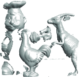
We used our RoPS together with the five feature descriptors (as detailed in Section 5.1.1) to perform object recognition. For feature descriptors that do not have a dedicated LRF, e.g., spin image, NormHist, LSP and THRIFT, the LRFs were defined using our proposed technique. The average number of detected feature points in an unsampled scene and a model were 985 and 1000, respectively.

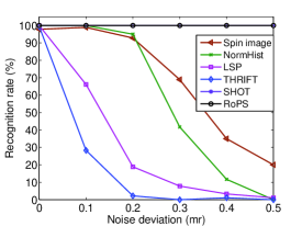
In order to evaluate the performance of the 3D object recognition algorithms on noisy data, we added a Gaussian noise with increasing standard deviation of 0.1mr, 0.2mr, 0.3mr, 0.4mr and 0.5mr to each scene data, the average recognition rates of the six algorithms on the 45 scenes are shown in Fig. 11(a). It can be seen that both RoPS and SHOT based algorithms achieved the best results, with recognition rates of 100% under all levels of noise. Spin image and NormHist based algorithms achieved recognition rates higher than 97% under low-level noise with deviations less than 0.1mr. However, their performance deteriorated sharply as the noise increased. While LSP and THRIFT based algorithms were very sensitive to noise.

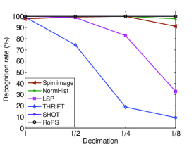
In order to evaluate the effectiveness of the 3D object recognition algorithms with respect to varying mesh resolution, the 45 noise free scenes were resampled to $\nicefrac{{1}}{{2}}$, $\nicefrac{{1}}{{4}}$ and $\nicefrac{{1}}{{8}}$ of their original mesh resolution. The average recognition rates on the 45 scenes with respect to different mesh resolutions are given in Fig. 11(b). It is shown that RoPS based algorithm achieved the best performance, obtaining 100% recognition rate under all levels of mesh decimation. It was followed by NormHist and spin image based algorithms. That is, they obtained recognition rates of 97.8% and 91.1% respectively in scenes with $\nicefrac{{1}}{{8}}$ of original mesh resolution.

7.2 Recognition Results on The UWA Dataset

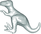
The UWA Dataset contains five 3D models and 50 real scenes. The scenes were generated by randomly placing four or five real objects together in a scene and scanned from a single viewpoint using a Minolta Vivid 910 scanner. An illustration of the five models is given in Fig. 12, and two sample scenes are shown in Figures 13(a) and (c).

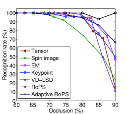
For the sake of consistency in comparison, RoPS based 3D object recognition experiments were performed on the same data as Mian et al. (2006b) and Bariya et al. (2012). Besides, the Rhino model was excluded from the recognition results, since it contained large holes and cannot be recognized by the spin image based algorithm in any of the scenes. Comparison was performed with a number of state-of-the-art algorithms, such as tensor (Mian et al., 2006b), spin image (Mian et al., 2006b), keypoint (Mian et al., 2010), VD-LSD (Taati and Greenspan, 2011) and EM based (Bariya et al., 2012) algorithms. Comparison results are shown in Fig. 14 with respect to varying levels of occlusion. The average number of detected feature points in a scene and a model were 2259 and 4247, respectively.

Occlusion is defined according to Johnson and Hebert (1999) as:

$$\textrm{occlusion}=\frac{\textrm{model surface patch area in scene}}{\textrm{total model surface area}}.$$ (23)

The ground truth occlusion values were automatically calculated for the correctly recognized objects and manually calculated for the objects which were not correctly recognized. As shown in Fig. 14, our RoPS based algorithm outperformed all the existing algorithms. It achieved a recognition rate of 100% with up to 80% occlusion, and a recognition rate of 93.1% even under 85% occlusion. The average recognition rate of our RoPS based algorithm was 98.8%, while the average recognition rate of spin image, tensor and EM based algorithms were 87.8%, 96.6% and 97.5% respectively, with up to 84% occlusion. The overall average recognition rate of our RoPS based algorithm was 98.9%. Moreover, no false positive occurred in the experiments when using our RoPS based algorithm, and only two out of the total 188 objects in the 50 scenes was not correctly recognized. These results confirm that our RoPS based algorithm is able to recognize objects in complex scenes in the presence of significant clutter, occlusion and mesh resolution variation.

Figure 14: Recognition rates on the UWA Dataset. (Figure best seen in color.)

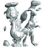
Two sample scenes and their corresponding recognition results are shown in Fig. 13. All objects were correctly recognized and their poses were accurately recovered except for the T-Rex in Fig. 13(d). The reason for the failure in Fig. 13(d) relates to the excessive occlusion of the T-Rex. It is highly occluded and the visible surface is sparsely distributed in several parts of the body rather than in a single area. Therefore, almost no reliable feature could be extracted from the object.

(a) Angle

(b) Big Bird

(c) Gnome

(d) Kid

(e) Zoe

Figure 15: The five models in the Queen’s Dataset.

(a) The first sample scene

(b) Our recognition result

(c) The second sample scene

(d) Our recognition result

Figure 16: Two sample scenes and our recognition results on the Queen’s dataset. The correctly recognized objects have been superimposed by their 3D complete models from the library. All objects were correctly recognized except for the Angle in (d). (Figure best seen in color.)

Note that, although we used a fixed support radius (i.e., $r$ = 15mr) for feature description throughout this paper, the proposed algorithm is generic, and different adaptive-scale keypoint detection methods can be seamlessly integrated within our RoPS descriptor. In order to further demonstrate the generic nature of our algorithm, we generated RoPS descriptors using the support radii estimated by the adaptive-scale method in (Mian et al., 2010). The recognition result is shown in Fig. 14. The recognition performance of the adaptive-scale RoPS based algorithm was better than that reported in (Mian et al., 2010), which means that our RoPS descriptor was more descriptive than the descriptor used in (Mian et al., 2010). It is also observed that the performance of adaptive-scale RoPS was marginally worse than the fixed-scale counterpart. This is because the errors of scale estimation adversely affected the performance of feature matching, and ultimately object recognition. That is, the corresponding points in a scene and model may have different estimated scales due to the estimation errors. As reported in (Tombari et al., 2013), the scale repeatability of the adaptive-scale detector in (Mian et al., 2010) were less than 85% and 60% on the Retrieval dataset and Random Views dataset, respectively.

7.3 Recognition Results on The Queen’s Dataset

The Queen’s Dataset contains five models and 80 real scenes. The 80 scenes were generated by randomly placing one, three, four or five of the models in a scene and scanned from a single viewpoint using a LIDAR sensor. The five models were generated by merging several range images of a single object. Since all scenes and models were represented in the form of pointclouds, we first converted them into triangular meshes in order to calculate the LRFs using our proposed technique. A scene pointcloud was converted by mapping the 3D pointcloud onto the 2D retina plane of the sensor and performing a 2D Delaunay triangulation over the mapped points. The 2D points and triangles were then mapped back to the 3D space, resulting in a triangular mesh. A model pointcloud was converted into a triangular mesh using the Marching Cubes algorithm (Guennebaud and Gross, 2007). An illustration of the five models is given in Fig. 15, and two sample scenes are shown in Figures 16(a) and (c).

Table 6: Recognition rates (%) on the Queen’s Dataset. The results of the tests on the full dataset containing 80 scenes are shown in parentheses. The others were tested on a subset dataset which contains 55 scenes. ‘NA’ indicates that the corresponding item is not available. The best results are in bold fonts.

Method	Angel	Big Bird	Gnome	Kid	Zoe	Average
RoPS	97.4 (97.9)	100.0 (100.0)	97.4 (97.9)	94.9 (95.8)	87.2 (85.4)	95.4 (95.4)
EM	NA (77.1)	NA (87.5)	NA (87.5)	NA (83.3)	NA (76.6)	81.9 (82.4)
VD-LSD(SQ)	89.7	100.0	70.5	84.6	71.8	83.8
VD-LSD(VQ)	56.4	97.4	69.2	51.3	64.1	67.7
3DSC	53.8	84.6	61.5	53.8	56.4	62.1
Spin image (impr.)	53.8	84.6	38.5	51.3	41.0	53.8
Spin image (orig.)	15.4	64.1	25.6	43.6	28.2	35.4
Spin image spherical (impr.)	53.8	74.4	38.5	61.5	43.6	54.4
Spin image spherical (orig.)	12.8	61.5	30.8	43.6	30.8	35.9

First, we performed object recognition using our RoPS based algorithm on the full dataset which contains 80 real scenes. The average number of detected feature points in a scene and a model were 3296 and 4993, respectively. The results are shown in parentheses in Table 6, with a comparison to the results given by Bariya et al. (2012). It can be seen that the average recognition rate of our algorithm is 95.4%, in contrast, the average recognition rate of the EM based algorithm is 82.4%. These results indicate that our algorithm is superior to the EM based algorithm although a complicated keypoint detection and scale selection strategy has been adopted by the EM based algorithm.

To make a direct comparison with the results given by Taati and Greenspan (2011), we performed our RoPS based 3D object recognition on the same subset dataset which contains 55 scenes. The results are given in Table 6, with comparisons to the results provided by two variants of VD-LSD, 3DSC and four variants of spin image. As shown in Table. 6, our average recognition rate was 95.4%, while the second best result achieved by VD-LSD (SQ) was 83.8%. The RoPS based algorithm achieved the best recognition rates for all the five models. More than 97% of the instances of Angle, Big Bird and Gnome were correctly recognized. Although RoPS’s recognition rate for Zoe was relatively low (i.e., 87.2%), it still outperformed the existing algorithms by a large margin, since the second best result achieved by VD-LSD (SQ) was 71.8%. Fig. 16 shows two sample scenes and our recognition results on the Queen’s Dataset. It can be seen that our RoPS based algorithm was able to recognize objects with large amounts of occlusion and clutter.

Note that, the Queen’s Dataset is more challenging than the UWA Dataset since the former is more noisy and the points are not uniformly distributed. That is the reason why the spin image based algorithm had a significant drop in the recognition performance when tested on the two datasets. Specifically, the average recognition rate of spin image based algorithm on the UWA Dataset was 87.8% while the best result on the Queen’s Dataset was only 54.4%. Similarly, a notable decrease of performance can also be found for the EM based algorithm, with 97.5% recognition rate for the UWA Dataset and 81.9% recognition rate for the Queen’s Dataset. However, our RoPS based algorithm was consistently effective and robust to different kinds of variations (including noise, varying mesh resolution and occlusion), it outperformed the existing algorithms and achieved comparable results in both datasets, obtaining a recognition rate of 98.9% on the UWA Dataset and 95.4% on the Queen’s Dataset.

We also performed a timing experiment to measure the average processing time to recognize each object in the scene. The experiment was conducted on a computer with a 3.16 GHz Intel Core2 Duo CPU and a 4GB RAM. The code was implemented in MATLAB without using any program optimization or parallel computing technique. The average computational time to detect feature points and calculate LRFs was 42.6s. The average computational time to generate RoPS descriptors was 7.2s. Feature matching consumed 46.6s, while the computational time for the transformation hypothesis generation was negligible. Finally, verification and segmentation cost 57.4s in average.

7.4 Recognition Results on The Ca’ Foscari Venezia Dataset

This dataset is composed of 20 models and 150 scenes. Each scene contains 3 to 5 objects in the presence of occlusion and clutter. Totally, there are 497 object instances in all scenes. This dataset has been released just recently. It is the largest available 3D object recognition dataset. It is also more challenging than many other datasets, containing several models with large flat and featureless areas, and several models which are very similar in shape (Rodolà et al., 2012).

Table 7: Precision and recall values on the Ca’ Foscari Venezia Dataset. The best results are in bold fonts.

		Armadillo	Bunny	Cat1	Centaur1	Chef	Chicken	Dog7	Dragon	Face
Precision	RoPS	97	100	100	100	100	97	100	100	100
	Game-theoretic	100	100	78	96	93	93	95	100	91
Recall	RoPS	100	100	44	100	100	100	91	100	100
	Game-theoretic	97	97	82	100	100	100	86	89	95
		Ganesha	Gorilla0	Horse7	Lioness13	Para	Rhino	T-Rex	Victoria3	Wolf2
Precision	RoPS	100	100	100	100	97	96	100	100	100
	Game-theoretic	89	95	97	88	97	91	97	83	82
Recall	RoPS	100	100	100	100	97	100	100	95	100
	Game-theoretic	100	91	100	100	94	91	97	83	95

The precision and recall values of RoPS based algorithm on this dataset is shown in Table 7, the results as reported in (Rodolà et al., 2012) are also reported for comparison. As in (Rodolà et al., 2012), two out of the 20 models were left out from the recognition tests and used as clutter. The average number of detected feature points in a scene and a model were 2210 and 5000, respectively. The RoPS based algorithm achieved better precision results compared to (Rodolà et al., 2012). The average precision of RoPS based algorithm was 99%, which was higher than (Rodolà et al., 2012) by a margin of 6%. Besides, the precision values of 14 individual models were as high as 100%.

The average recall of RoPS based algorithm was 96%, in contrast, the average recall of (Rodolà et al., 2012) was 95%. Moreover, RoPS based algorithm achieved equal or better recall values on 17 individual models out of the 18 models. Note that, SHOT descriptors and a game-theoretic framework is used in (Rodolà et al., 2012) for 3D object recognition. It is observed that our RoPS based algorithm performed better than SHOT based algorithm on this Dataset.

In summary, the superior performance of our RoPS based 3D object recognition algorithm is due to several reasons. First, the highly descriptiveness and strong robustness of our RoPS feature descriptor improve the accuracy of feature matching and therefore boost the performance of 3D object recognition. Second, the unique, repeatable and robust LRF enables the estimation of a rigid transformation from a single feature correspondence, which therefore reduces the errors of transformation hypotheses. This is because the probability of selecting only one correct feature correspondence is much higher than the probability of selecting three correct feature correspondences. Moreover, our proposed hierarchical object recognition algorithm enables object recognition to be performed in an effective and efficient manner.

8 Conclusion

In this paper, we proposed a novel RoPS feature descriptor for 3D local surface description, and a new hierarchical RoPS based algorithm for 3D object recognition. The RoPS feature descriptor is generated by rotationally projecting the neighboring points around a feature point onto three coordinate planes and calculating the statistics of the distribution of the projected points. We also proposed a novel LRF by calculating the scatter matrix of all points lying on the local surface rather than just mesh vertices. The unique and highly repeatable LRF facilitates the effectiveness and robustness of the RoPS descriptor.

We performed a set of experiments to assess our RoPS feature descriptor with respect to a set of different nuisances including noise, varying mesh resolution and holes. Comparative experimental results show that our RoPS descriptor outperforms the state-of-the-art methods, obtaining high descriptiveness and strong robustness to noise, varying mesh resolution and other deformations.

Moreover, we performed extensive experiments for 3D object recognition in complex scenes in the presence of noise, varying mesh resolution, clutter and occlusion. Experimental results on the Bologna Dataset show that our RoPS based algorithm is very effective and robust to noise and mesh resolution variation. Experimental results on the UWA Dataset show that RoPS based algorithm is very robust to occlusion and outperforms existing algorithms. The recognition results achieved on the Queen’s Dataset show that our algorithm outperforms the state-of-the-art algorithms by a large margin. The RoPS based algorithm was further tested on the largest available 3D object recognition dataset (i.e., the Ca’ Foscari Venezia Dataset), reporting superior results. Overall, our algorithm has achieved significant improvements over the existing 3D object recognition algorithms when tested on the same dataset.

Interesting future research directions include the extension of the proposed RoPS feature to encode both geometric and photometric information. Integrating geometric and photometric cues would be beneficial for the recognition of 3D objects with poor geometric but rich photometric features (e.g., a flat or spherical surface). Another direction is to adopt our RoPS descriptors to perform 3D shape retrieval on a large scale 3D shape corpus, e.g., the SHREC Datasets (Bronstein et al., 2010b).